Population Balance Application in TiO₂ Particle Deagglomeration Process Modeling

Abstract

The deagglomeration of titanium-dioxide powder in water suspension performed in a stirring tank was investigated. Owing to the widespread applications of the deagglomeration process and titanium dioxide powder, new, more efficient devices and methods of predicting the process result are highly needed. A brief literature review of the application process, the device used, and process mechanism is presented herein. In the experiments, deagglomeration of the titanium dioxide suspension was performed. The change in particle size distribution in time was investigated for different impeller geometries and rotational speeds. The modification of impeller geometry allowed the improvement of the process of solid particle breakage. In the modelling part, numerical simulations of the chosen impeller geometries were performed using computational-fluid-dynamics (CFD) methods whereby the flow field, hydrodynamic stresses, and other useful parameters were calculated. Finally, based on the simulation results, the population-balance with a mechanistic model of suspension flow was developed. Model predictions of the change in particle size showed good agreement with the experimental data. Using the presented method in the process design allowed the prediction of the product size and the comparison of the efficiency of different impeller geometries.

1. Introduction

Breaking up solid particles is a widely used industrial process, especially in the paint and coating industries [1,2]. Other industries where this process is used are the food, medicine, and chemical industries. Typical applications of the process of breaking up particles are presented in [3]. The final particle-size distribution has a significant influence on the product properties; therefore, planning and supervising process efficiency and performance are highly important. The product performance depends not only on its ingredients but also on its preparation method [4]. Titanium dioxide is commonly applied as a paint and coating base in the aqueous suspension of solid particles. Further, owing to its photocatalytic properties and high refractive index, titanium dioxide has applications in the optical industry [5]. With regard to the technical quality of the substance, titanium dioxide has a white-powder form and consists of clusters with a complex structure. The creation of agglomerates involves several stages, including the nucleation of primary particles, the sticking into primary aggregates, and the formation of clusters called agglomerates [6]. Primary particles in aggregates are connected to each other via strong crystal bounds, which cannot be broken by the flow [7]. Connections in agglomerates are established by adhesive forces, which are weaker than chemical bonds; therefore, they can be easily destroyed by shear forces [8]. Before titanium-dioxide powder can be used as a paint, its structure has to be broken into smaller parts. This process is performed in special devices such as ball mills [9,10] and high shear mixers [11,12]. Ultrasonication [5,13] and high-pressure nozzles [13,14,15,16] are often applied. The performance features of those devices can be found in [17]. According to this work, an agitated vessel equipped with a Rushton turbine can generate energy dissipation in a range from 0.1 to 100 W/kg, valve homogenizer at about 10⁸ W/kg, and ultrasonication at about 10⁹ W/kg. The phenomenon of breaking up solid-particle agglomerates in suspensions occurs when shear stresses generated in the liquid are stronger than the cluster tensile strength [18]. The size of a particle, created during breakage, depends on the breakage mechanism. Three main possibilities of fragmentation are considered: shattering, rupture, and erosion [8]. In deagglomeration, all these mechanisms occur simultaneously. An investigation of the changes in particle-size distribution over time enables us to identify the dominant process.

In this study, experiments and modelling of the deagglomeration of titanium dioxide powder conducted in a stirring tank equipped with high-shear impellers were investigated. Based on the division proposed in [19], particles larger than 1 µm are named suspended particles and those smaller are called colloidal particles. In this study, suspended particles were investigated. The industrial application typically consists of three stages. The first is powder wetting, which removes air from the pores and allows the creation of a suspension. The second is deagglomeration, which imparts the desired properties to the suspension. The third is particle stabilization, which prevents the reagglomeration of particles created during the breakage [20]. The deagglomeration process was performed in a tank mixer equipped with three types of high-shear impellers for two rotational speeds. CFD simulations were performed for three impeller geometries and three rotational speeds. Based on them, it was possible to divide the fluid zone into some specific regions and check their turbulence properties. Those values were applied in population-balance calculations. Furthermore, simulations allowed us to investigate the liquid path in the tank and its velocity, localize death zones, analyze the surface curvature, and calculate the mixing power and liquid mass flow rates near the impeller. Those values allowed us to characterize the process and estimate the efficiency of each impeller type. As mentioned earlier, turbulence properties were applied in population-balance calculations. For solving the population-balance equations, the direct quadrature method of moment (DQMOM) was used. This method was developed by [21]. It is based on the quadrature method of moment (QMOM) described in [22]. The application of this method for solving aggregation and breakage problems is detailed in [23].

2. Experiments

Experiments were carried out in an unbaffled tank mixer. Its diameter was $T=240$ mm. The device is presented in Figure 1. This tank was equipped with a cooling jacket, which allows the prevention of overheating the suspension, and clean water was used as a coolant. In all experiments, an impeller was placed on the same level above the tank bottom $h=T/12$. The suspension height was the same in every experiment, equal to $0.48T$. Three types of the impeller with diameters equal to $T/2$ were used. All impellers are presented in Figure 2. The geometry of impellers was new or hybrid, based on publications of other authors [24,25]. In case 1, the impeller had the shape of a saw blade. It was a flat disc with sawtooth cuts on its edge. The number of teeth was the same for every case, equal to 18. The impeller in case 2 was a modification of the previous case. In every tooth, triangular cuts were made. Five cylindrical holes of diameter $d$ were also made. These holes were made on a circumference of diameter $D_2$ in equal distance. In the last case, described as case 3, the impeller was made similar to that in case 2. Triangular cuts were also made. Instead of cylindrical holes on the circumference of diameter $D_2$, gaps were made. Gaps were not drilled perpendicular to the impeller’s face but inclined at $45$°. The thickness of discs was the same for each impeller, equal to $1.5$ mm.

The direction of rotation was clockwise, relative to that presented in Figure 2. For every impeller, experiments were carried out for two values of rotational speed.

The titanium dioxide used in experiments had a rutile structure. The concentration of the solid phase was 40% of the mass mixture. As a continuous phase, ultra-pure demineralized water was used. Its conductance was no higher than 0.05 µS. Samples were analyzed on the particle size analyzer LS 13,320 Beckman Coulter. This device integrates two measurement techniques: laser diffraction (LD) and polarization intensity differential scattering (PIDS). The total size range measured by the apparatus is from 0.04 to 2000 µm.

The deagglomeration process lasted 60 min. Samples were taken during the process without interrupting the working of the impeller. After that, ultra-pure water was added to samples in order to reduce the agglomeration of particles. For every measurement set, at least eight samples were taken. Due to the fast change in size at the beginning of the process, more samples were taken in the first ten minutes of the working of the impeller.

3. Process Simulations

3.1. System Geometry

The geometry in simulations represented the system used in the experiments. The geometry represented the internal part of the tank, and it consisted of volume available for fluid. To reduce the number of cells in the geometry, 1/6 of the domain was simulated. A periodic boundary condition was applied. Based on the geometry evaluation, meshes were created. The numbers of cells were 1,345,269, 1,406,469, and 2,020,213 for mixers in cases 1, 2, and 3, respectively. The mesh for which the results did not depend on the number of cells was chosen. The numerical mesh was generated using ANSYS Fluent Meshing 2020. The mesh was refined near the impeller. In this region, tetrahedral cells were used with sizes up to 0.5 mm. In the fluid core, hexahedral cells were applied, with sizes up to 3 mm. To check mesh independence, an average value of turbulence energy dissipation rate at the highest impeller speed tested was used. It was observed that the results of the computations were not sensitive to a further increase in the number of cells, i.e., the average energy dissipation rate value was constant despite a further increase in mesh density. On the tank wall, a stationary wall with a no-slip boundary condition was applied. On the shaft and the impeller moving wall, specific rotational speed and no-slip boundary conditions were applied.

The coupled solver was used for the pressure–velocity coupling, and second-order discretization schemes were used for all variables to minimize numerical diffusion effects.

3.2. Environment and Models

Simulations were performed in Fluent 2020 R2 software. The flow field was calculated using a steady-state simulation of the fluid flow. Owing to the high values of fluid velocity near the impeller turbulence model, a realizable $k-\epsilon$ was used. Results were obtained with second-order discretization. Owing to the high values of rotational speed, the liquid surface is curved. Therefore, it is necessary to inspect how large this deformation is. If the central vortex reaches the mixer disc and the impeller is not fully submerged in the liquid, less power is transferred into the liquid. The multiphase model must be applied. For the dynamics of the liquid surface, the volume-of-fluid (VOF) multiphase model is suitable. The impeller movement was applied by the multiple-reference-frame (MRF) model. For each impeller, the case simulation was performed for three values of rotational speed: 500, 1200, and 3000 rpm.

3.3. Suspension Properties

The viscosity of the titanium dioxide suspension was investigated in [26,27] with respect to the temperature, pH, and solid concentration. The study results indicate that the rheological properties of the TiO₂ suspension could be approximated by the Einstein equation for dilute suspensions (below 5% volume concentration). For higher solid-phase concentrations, the Casson, Quemada, and Herschel–Bulkley models can be employed. The research conducted on titanium-dioxide powder, used in this study, showed that the suspension behaves as a shear-thinning liquid. The mixture of solid particles suspended in water was simulated as a homogenous substance, the rheological behavior of which can be expressed by the Carreau model [28] given by the following equation:

$$\mu ={\mu }_{\infty }+\left({\mu }_0-{\mu }_{\infty }\right){\left[1+{\left(\lambda \dot{\gamma }\right)}^2\right]}^{\frac{n-1}{2}},$$

(1)

where $\mu$ [Pa∙s] is the apparent viscosity and $\dot{\gamma }$ [s⁻¹] is the shear rate. Based on the experiments, the model constants were obtained. Measurements were made using the Anton Paar MCR 302 rheometer in the plate–plate system and the coaxial cylinder system. The viscosity at an infinite shear rate was ${\mu }_{\infty }=14.09$ Pa·s and that at a zero shear rate was ${\mu }_0=0.11$ Pa·s; the flow index was $n=0.1$ and the relaxation time was $\lambda =1.73$ s. The application of the homogenous model assumes that sedimentation does not occur.

3.4. Suspension Volume Fraction Profiles

The results of the liquid volume fraction $\mathsf{\Phi }$ [–] in the liquid–gas system obtained via simulation for case 3 are presented in Figure 3a–c. The analysis indicates that for the lowest value of rotational speed, the impeller did not cause surface deformation, implying that the impeller did not generate stresses high enough to decrease the viscosity below the value necessary to cause the surface deformation. This phenomenon can be observed in the apparent viscosity $\mu$ [Pa∙s] profiles in Figure 3d–f. For rotational speeds of 1200 and 3000 rpm, centrifugal forces caused such strong deformations in the liquid surface that the impeller was not fully submerged. This caused a spreading bubble in the suspension and decreased the amount of energy transferred from the impeller to the liquid, compared to that in the case of full submergence. The results obtained for the impeller in case 2 were similar.

3.5. Suspension Velocity

The numerical simulation allowed us to investigate the paths of liquid elements, their velocities, the formation of circulation loops, and the creation of dead zones. The results of cases 2 and 3 are presented in Figure 4 as a vector diagram. All the vectors are projected on the section plane. The vectors are equal in length, and their colors represent the velocity magnitude. The figure diagrams show the formation of circulation loops in the tank. The vectors show that there were two main regions of circulation. The first one was placed between the impeller and the tank wall. This loop was largest; the particles were lifted from the bottom and directed toward the impeller. The second circulation loop was placed below the impeller and caused movement of the suspension in this region. In Figure 4a,d, it can be observed that the stream of liquid near the impeller was splitting, and it flowed in two regions: one toward the larger circulation loop and the other under the impeller. The analysis also shows that in diagrams (b), (e), and (f) in the corner of the tank, the liquid had reversed circulation, compared to that under lower rotation speeds. Further, the fluid velocity in this region was very low. This can represent a stagnation zone. In this region, the suspension did not make any contact with the impeller, and as a result, particles were not crushed. A similar phenomenon can be observed in diagram (c), but in this case, the circulation loop was larger and the fluid velocity was much higher, thus allowing for the mixing of fluid elements.

4. Mechanistic Model

To predict the particle-size changes over time in the tank, population-balance methods were employed. Methods of describing the agglomeration and deagglomeration processes are presented in [23]. To solve the population-balance equations in this case, the direct quadrature method of moments was applied. The details of this method are presented in [21]. In this paper, only the deagglomeration process was considered and agglomeration was neglected. Due to low values of energy dissipation rate for 500 rpm, only higher values of rotational speed were involved in population balance computations.

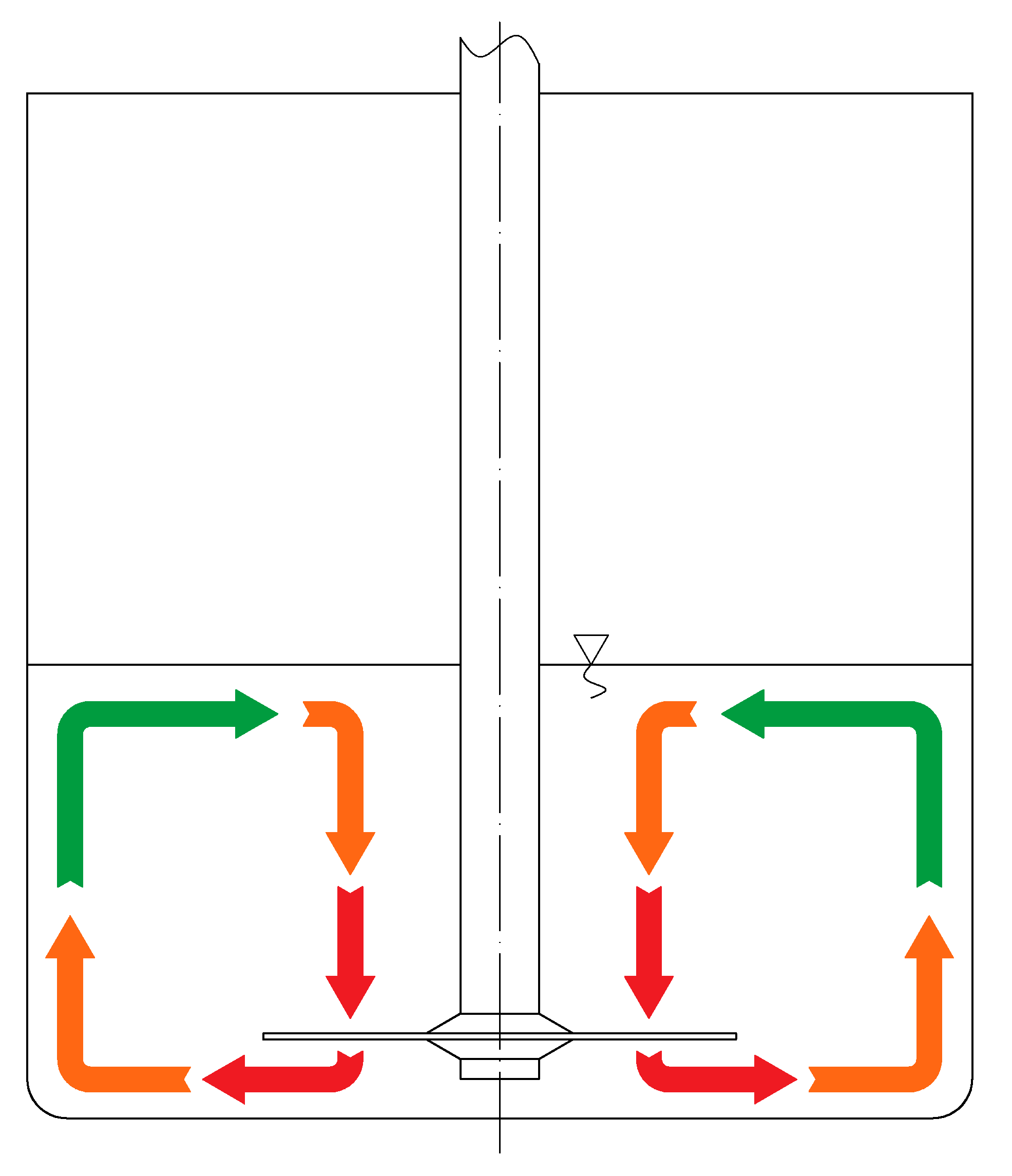
Particle clusters break as a result of hydrodynamic stresses generated in the liquid by the power input of an impeller. The values of those stresses can be evaluated via dimensionless analysis. This expression includes the turbulence energy dissipation rate, which can be calculated from the CFD simulation. To simplify this case, a mechanistic model was applied. In the tank domain, three characteristic zones were selected and numbered I, II, and III. The division criterion was the energy dissipation rate, $\epsilon$ [m²·s⁻³]. In zone I, the energy dissipation rate was higher than the average over the whole tank (i.e., $\epsilon >\overline{\epsilon }$). In zone II, $\epsilon$ was lower than the average but higher than the critical value, above which the breakage process begins (i.e., ${\epsilon }_{cr}<\epsilon <\overline{\epsilon }$). In zone III, the energy dissipation rate was lower than the critical rate (i.e., $\epsilon <{\epsilon }_{cr}$); therefore, deagglomeration did not occur in this region. The Fluent software allowed us to calculate the mass flow rate of the liquid near the impeller. The flow rate and zone volumes allowed us to calculate the residence time of the fluid element there. The energy dissipation rate was the average in each zone.

The following assumptions were made in the mechanistic model:

• Every fluid element is tracked in the Lagrangian way;
• Every fluid element has the same residence time in the selected zone;
• Fluid elements are completely segregated and do not mix with each other;
• Energy dissipation rates in the zones are constant;
• Particles do not aggregate or agglomerate;

In Figure 5, the liquid circulation through the dissipation zones is presented. The red, orange, and green arrows represent the flows through zones I, II, and III, respectively. The residence time and average energy dissipation rate are presented in

Table 1. Averaged energy dissipation rate and residence time.

Impller Type	Rotation Speed [rpm]	$\overline{\mathit{\epsilon }}$ in Zone I [m2·s−3]	$\overline{\mathit{\epsilon }}$ in Zone II [m2·s−3]	τI [s]	τII [s]	τIII [s]
Impeller 1	1200	15.11	0.8160	0.09	0.39	0.82
	3000	76.73	1.870	0.20	2.14	0.36
Impeller 2	1200	9.023	0.8919	0.33	0.80	0.79
	3000	40.36	1.974	0.47	1.23	0.36
Impeller 3	1200	22.29	0.8166	0.19	0.80	0.64
	3000	408.1	7.541	0.19	0.39	0.06

.

The application of DQMOM methods allows us to solve the population-balance equations with simple linear algebra; source-term specifications for equations are required. Owing to the assumption of negligible agglomeration effects, only breakage terms need to be defined. The population-balance equation for agglomerate breakage is given by the following formula [18]:

$$\frac{\partial f\left(L,\mathit{x},t\right)}{\partial t}+{\displaystyle \sum }_{i=0}^3\frac{\partial \left[u_{p,i}\left(L,\mathit{x},t\right)f\left(L,\mathit{x},t\right)\right]}{\partial x_i}+\frac{\partial \left[G\left(L,\mathit{x},t\right)f\left(L,\mathit{x},t\right)\right]}{\partial L}=B^b\left(L,\mathit{x},t\right)+D^b\left(L,\mathit{x},t\right),$$

(2)

where $f$ is the number density function, $u_{p,i}$ is the particle velocity in the $i$ direction, $\mathit{x}$ is the position vector, $t$ is the time coordinate, $G$ is the particle linear growth rate, and $L$ is the characteristic length of a particle.

$B^b$ and $D^b$ are birth and death rate functions, respectively, defined by

$$B^b\left(L,\mathit{x},t\right)=\underset{0}{\overset{\infty }{{\displaystyle \int }}}\mathsf{\Gamma }\left(\lambda \right)b\left(L|\lambda \right)f\left(\lambda ,\mathit{x},t\right)d\lambda ,$$

(3)

$$D^b\left(L,\mathit{x},t\right)=\mathsf{\Gamma }\left(L\right)f\left(L,\mathit{x},t\right),$$

(4)

where $b\left(L|\lambda \right)$ is a fragment distribution function that describes the number and size of particles $L$. created from the breakage of agglomerates of size $\lambda$. As mentioned earlier, the deagglomeration mechanism that dominates the process is shattering. For this mechanism, the fragment-distribution function is defined by the following equation:

$$b\left(L|\lambda \right)=N\left(\lambda \right)·\delta \left(L-L_a\right),$$

(5)

where $\delta \left(L-L_a\right)$ is the Dirac’s delta with a parameter $L_a$ size, which represents the aggregate size. $N\left(\lambda \right)$ is the number of aggregates in the agglomerate of size $\lambda$. This value can be evaluated by [14]:

$$N\left(\lambda \right)={\left(\frac{k_v}{k_{va}}\right)}^{\frac{D_f}{3}}{\left(\frac{\lambda }{L_a}\right)}^{D_f},$$

(6)

where k_v and k_va are the shape factors of agglomerates and aggregates, respectively. D_f is the fractal dimension of the agglomerate.

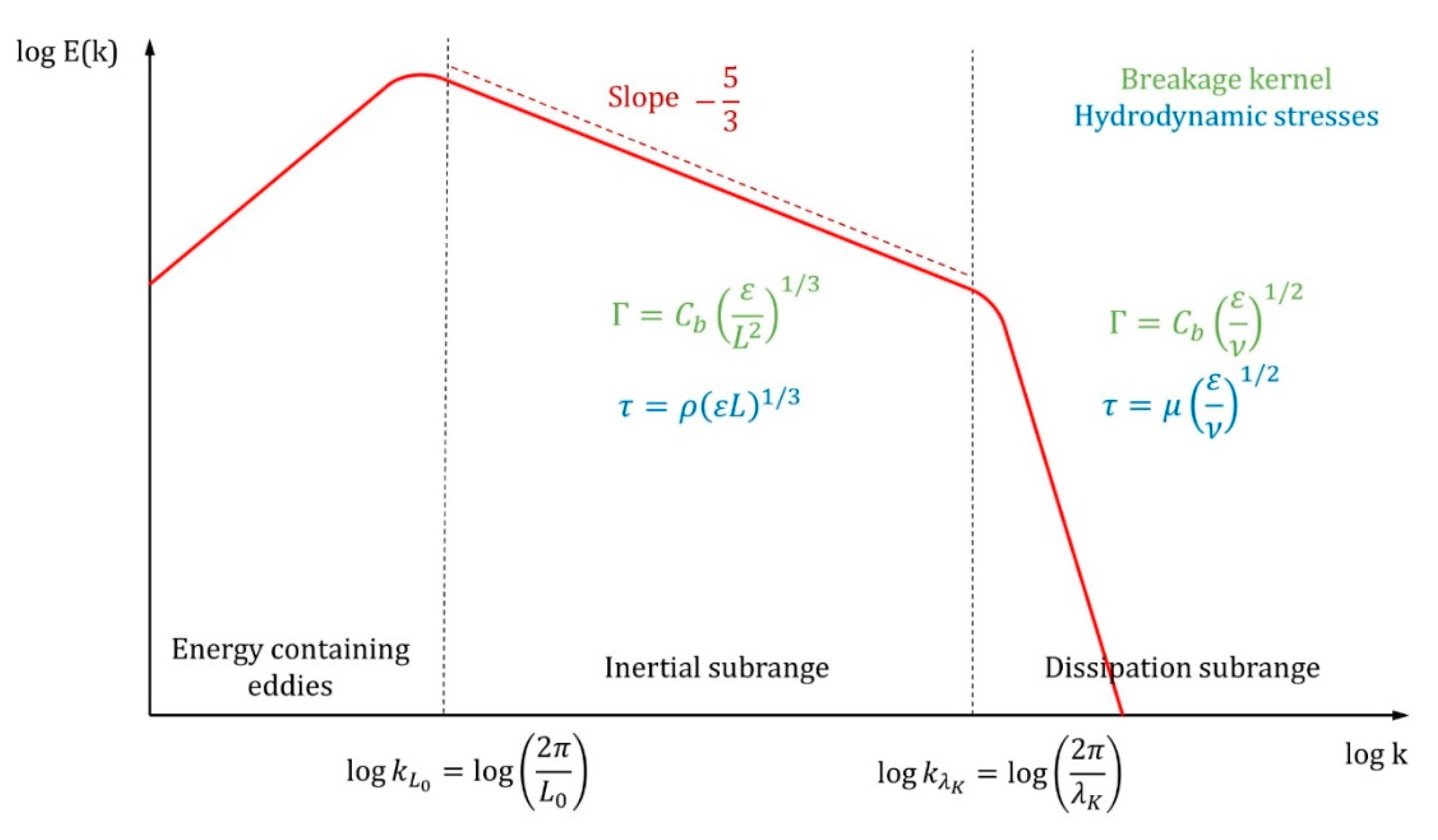
Function Γ is a breakage kernel; it describes the frequency of deagglomeration events. It depends on the fluid properties, flow pattern, and particle properties, as reported in [29]. Breakage occurs when hydrodynamic stresses are greater than the agglomerate tensile strength. This function is defined in two ways. The division criteria are based on the Kolmogorov length microscale [30], given by

$${\lambda }_K={\left(\frac{{\nu }^3}{\epsilon }\right)}^{\frac{1}{4}},$$

(7)

where $\nu$ [m²·s⁻¹] is the kinematic viscosity of the fluid and $\epsilon$ [m²·s⁻³] is the turbulence energy dissipation rate. For particles larger than the Kolmogorov microscale, $L>{\lambda }_k$, deagglomeration occurs in the inertial subrange of turbulence spectrum [13]. The kernel is given by

$$\mathsf{\Gamma }=\{\begin{array}{c}{C}_b{\left(\frac{\epsilon }{L^2}\right)}^{1/3} if \rho {\left(\epsilon L\right)}^{1/3}>\sigma \\ 0 if \rho {\left(\epsilon L\right)}^{1/3}\le \sigma \end{array}.$$

(8)

where $\rho$ is the fluid density. $\rho {\left(\epsilon L\right)}^{1/3}$ describes the hydrodynamic stresses in the inertial subrange of the turbulence spectrum. ${\left(\frac{\epsilon }{L^2}\right)}^{1/3}$ represents the frequency of turbulence events. For particles smaller than or equal to the Kolmogorov microscale, $L\le {\lambda }_K$, breakage occurs in the dissipation subrange of the turbulence spectrum. In this case, the breakage kernel, based on the inversion of the Kolmogorov time scale, is given by

$$\mathsf{\Gamma }=\{\begin{array}{c}{C}_b{\left(\frac{\epsilon }{\nu }\right)}^{1/2} if \mu {\left(\frac{\epsilon }{\nu }\right)}^{1/2}>\sigma \\ 0 if \mu {\left(\frac{\epsilon }{\nu }\right)}^{1/2}\le \sigma \end{array}.$$

(9)

In Equations (8) and (9), $C_b$ is a constant. This phenomenon is illustrated in Figure 6.

In Figure 6, $E$ is the kinetic energy of the turbulence, $k$ is the wave number, $L_0$ is the characteristic length of the largest eddies in the inertial subrange, ${\lambda }_K$ is the Kolmogorov length scale of the eddies, and $\mu$ and $\nu$ are the dynamic and kinematic viscosities of the continuous phase, respectively. The agglomerate tensile strength is a result of interactions between its components; it is a result of the occurrence of two forces: attraction and repulsion. The first one is caused by van der Waals forces. The second one is caused by the electrostatic double layer near the particle surface [31]. The tensile strength in fractal clusters of particles was investigated and reported in [32]. For agglomerates, this value is given by the following formula:

$${\sigma }_T=1.1\frac{\left(1-ϵ\right)}{ϵ}\frac{F}{L_a^2},$$

(10)

where $ϵ$ is the cluster porosity, $L_a$ is the characteristic length of aggregates, and $F$ is the bounding force between agglomerate components. Its value is the sum of attractive and repulsive forces. In this case, only attractive effects are included. The attractive forces are given by

$$F=\frac{Ha{L}_0}{48H^2},$$

(11)

where $Ha$ is the Hamaker constant, $L_0$ is the characteristic size of primary particles, and $H$ is the surface-to-surface distance.

The agglomerate porosity, $ϵ$, is given by the following formula presented in [13]:

$$ϵ\left(L\right)=1-\frac{D_f}{3}\frac{k_v^{\left(\frac{D_f}{3}\right)-1}}{k_{va}^{\left(\frac{D_f}{3}\right)-1}}{\left(\frac{L}{L_a}\right)}^{D_f-3}.$$

(12)

To discover the morphology of the substance, scanning electron microscope images were obtained on two devices. Images of particles before deagglomeration were obtained on the Hitachi SU8230. The accelerating voltage of this device was 10 kV. These samples were not coated before the examination. Images of particles after deagglomeration were obtained on the Phenom G1 from PhoenomWorld company. The accelerating voltage of the device was 5 kV. Before the examination, samples were prepared to prevent charging and were coated with a mixture of gold and palladium (80% of gold and 20% of palladium atomic rate). The coating-layer thickness was approximately 8 nm. This coating was developed by the Q150 T Sputter Turbomolecular pumped coater from the Quorum company. The samples in Figure 7a,b present the raw material before stirring. The samples presented in Figure 7c,d were deagglomerated as a water suspension by a high-shear mixer for 60 min.

The analysis results for the images, presented in Figure 7, suggest that the aggregates and agglomerates had a fractal structure. Agglomerates of titanium dioxide are presented in images (a) and (b). The aggregates presented in images (c) and (d) consisted of smaller particles of submicron sizes. These clusters also had a porous structure. Image (c) shows suspension compounds at 5000× magnification. It shows the aggregates, which were torn from the larger structure. The second image shows the titanium-dioxide aggregate at 20,000× magnification. Based on the SEM images for further calculations, the characteristic size of the aggregates was equal to $L_a$ = 4 µm.

To define the agglomerate behavior during the breakage, the structures of those clusters were described by a model similar to that presented in [18]. The parameters required by the model were taken from the mentioned work and were equal; $k_v$ = π/6, $k_{va}$ = π/6, $D_f$ = 2.85, $\rho$ = 998.2 kg·m⁻³, $\mu$ = 1.003 × 10⁻³ Pa·s, $Ha$ = 5 × 10⁻²¹ J, $H$ = 1 nm, and $L_0$ = 20 nm. In the breakage, the kernel constant is equal ($C_b$ = 1 × 10⁻⁶). This value is lower than 1. This means that not every turbulent event can break up a solid particle. In reference [18], the authors suggested that this is a result of the intermittency phenomenon. The critical value of energy dissipation rate was found to be ${\epsilon }_{cr}$ = 0.178 m²·s⁻³ in this case.

5. Results

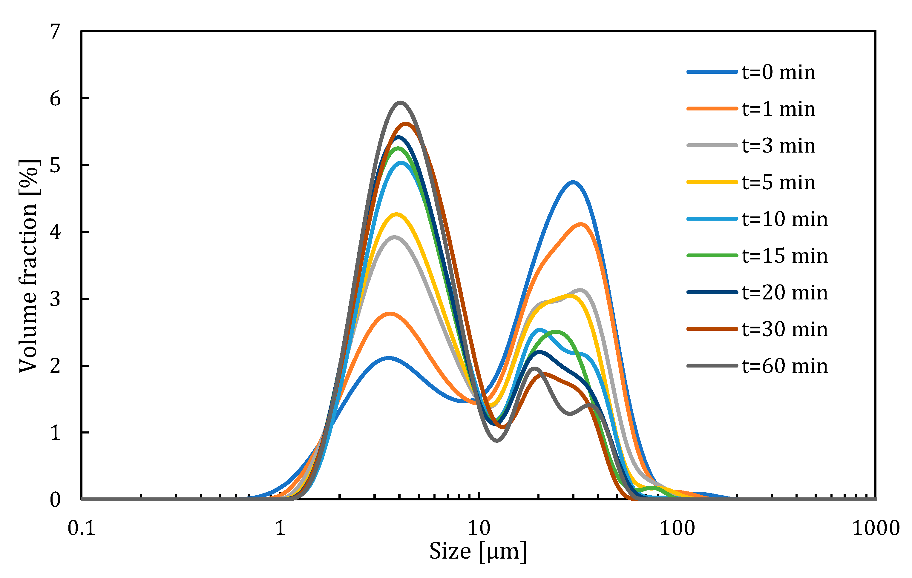
As a result of the experimental study, particle size distribution changes in time have been obtained. The results for impeller 1 for a rotation speed of 1200 rpm are presented in Figure 8. The analysis shows that this product consisted of two populations of particles. During the deagglomeration process, the population of larger particles shrank and the population of smaller particles grew. Based on the division proposed in [33], in this system, the shattering deagglomeration mechanism dominated.

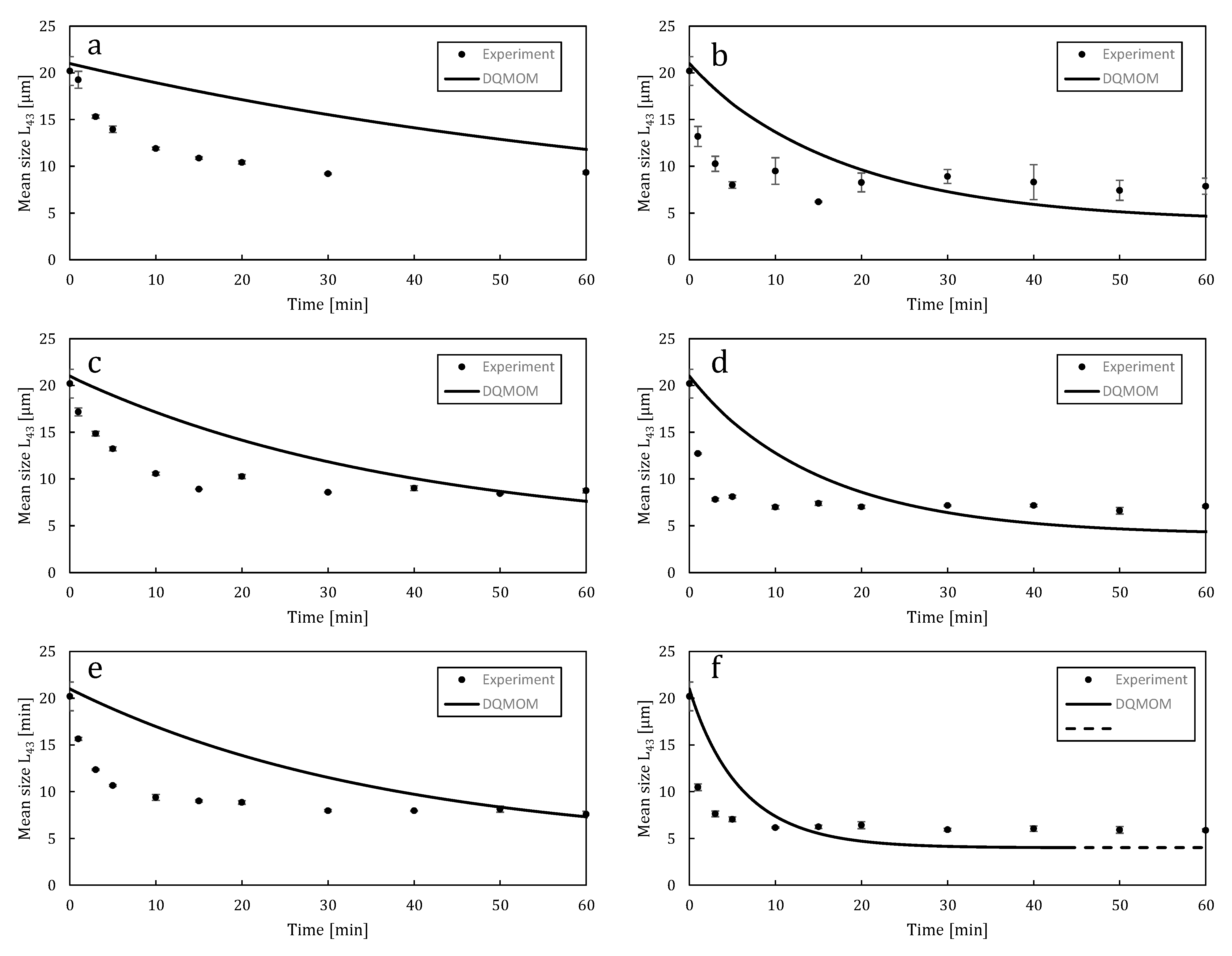
The results of the mechanistic-model application are presented in Figure 9. The residence time of the liquid element in each zone was found from the zone volume and flow rate near the impeller. Those values were calculated from the CFD results. The mean size of the particles in the system $L_{43}$ was calculated based on 4th- and 3rd-order statistical moments $m_4$ and $m_3$, respectively.

$$L_{43}=\frac{m_4}{m_3}.$$

(13)

The experimental study showed that impeller 3 had the highest ability of deagglomeration. For rotational speeds of 1200 and 3000 rpm, this impeller allowed the smallest final size of the particles to be obtained. This impeller characterized the fastest particle size drop. It shows that the application of this impeller allowed the required particle size to be obtained faster than for other geometries. It shortened the time of the deagglomeration process. The application of this allowed a smaller final size of the particles to be obtained than for other studied geometries. This shows that impeller 3 for the rotational speed 3000 rpm allowed the obtaining of a mean size of 2 µm smaller particles than those of unmodified geometry 1. In addition, for the rotational speed of 1200 rpm, the application of impeller 3 allowed a particle size of 7.589 µm to be obtained. Using impeller 1 for a rotational speed of 3000 rpm allowed a particle size of 7.871 µm to be obtained after 60 min of deagglomeration.

An analysis of Figure 9 showed good agreement of the experimental data with the population balance methods combined with a mechanistic model of suspension flow. This shows that this method can be applied to predict the results of deagglomeration in the design process. In the first stage of deagglomeration, the particle sizes obtained by experiments were smaller than those predicted by the model. This suggests that in the deagglomeration process for larger agglomerates, a different mechanism of deagglomeration dominated than for smaller one. A potential method for model improvement is to apply a rapid mechanism of deagglomeration for larger particles and a second, slower mechanism for small agglomerates. In Figure 9f, model prediction ended after 40 min. This was caused by numerical issues. In long or intensive deagglomeration, Dirac deltas used in the quadrature approximation approached the size of the aggregate. It caused the numeric matrix solved in the DQMOM method to be near to the singular matrix, and further calculation was not necessary, because the model reached the final obtainable size possible.

6. Discussion

This experimental study showed that the application of impeller 3 allowed smaller particles than those of other studied geometries to be obtained. In addition, this impeller characterized the fastest particle size drop in time. This suggests that the application of this type of impeller allowed the desirable size of the product to be obtained faster than for other geometries and, consequently, with less energy consumption.

The application of CFD methods and the volume of the fluid multiphase model allowed us to successfully reconstruct the conditions in a tank during particle deagglomeration. It also allowed us to investigate the mixing power that enabled the inspection of the power consumption of the process. CFD simulations indicated the parameters that were useful in the population-balance model; they allowed us to find the properties of zones separated in the mechanistic model. An investigation of the liquid path in the tank, based on the simulation results, indicated the dead zones, which can cause inhomogeneities in the product. The application of population-balance equations in the mechanistic model of suspension flow in the system provided information about the tendencies of breakage ability. Combining computational fluid dynamics and population balance gave a useful tool in the designing process. It allowed the prediction of particle sizes after deagglomeration with good approximation. This approach required less time and hardware resources than the implementation of the population balance equation into the CFD code and its solution in every cell in the tank domain. The application of a mechanistic model of suspension flow simplified the population balance equation, reducing it to a one-dimensional problem—solving it only for the time variable. The computational time needed to obtain the change in particle size with time for 3600 circulations of fluid elements for impeller 3 for 1200 rpm was 174.8 ± 1.1 s, averaged over five measurements. The calculation was made on an AMD Ryzen 7 3700X CPU, on a single core with a frequency up to 4.4 GHz using the Matlab^® platform. Differential equations were solved using the implemented algorithm ode45, with a fixed time step. Using an algorithm with an adaptive time step, for example, ode15s, could speed up calculations. The CFD computation required to obtain the results took 48 h, including post-processing, the use of a computing cluster, and parallel computation on a 10-core AMD Opteron 6284 SE CPU.

The proposed method is fast and accurate and can be successfully applied to the selection of mixer geometries in industrial applications. The limitation of this method is connected with the breakage kernel constant C_b that has to be found based on the experiment. The value of this constant will be different for each type of substance. It implicates the necessity of experimental study on each type of substance or literature search. Furthermore, we observed that in the first stage of deagglomeration, the particle sizes obtained by experiments were smaller than those predicted by the model. This suggests that in the deagglomeration process for larger agglomerates, a different mechanism of deagglomeration dominates than for the smaller one. The identification of the breaking mechanisms requires more experimental studies and can be considered as a further development of our research.

References

1. Hassan, A.; Hassan, A.; Borsinger, G. High Shear Process for Producing Micronized Waxes. U.S. Patent Application No. 8,450,539 B2, 28 May 2013. [Google Scholar]
2. Lee, F.P.-H.; Wong, R.W.-N.; van Kao, S. Processes for Preparing Phase Change Inks. U.S. Patent Application No. 7,556,679 B2, 7 July 2009. [Google Scholar]
3. Zhang, J.; Xu, S.; Li, W. High shear mixers: A review of typical applications and studies on power draw, flow pattern, energy dissipation and transfer properties. Chem. Eng. Process. Process Intensif. 2012, 57–58, 25–41. [Google Scholar] [CrossRef]
4. Rodgers, T.L.; Cooke, M.; Siperstein, F.R.; Kowalski, A. Mixing and dissolution times for a cowles disk agitator in large-scale emulsion preparation. Ind. Eng. Chem. Res. 2009, 48, 6859–6868. [Google Scholar] [CrossRef]
5. Mandzy, N.; Grulke, E.; Druffel, T. Breakage of TiO2 agglomerates in electrostatically stabilized aqueous dispersions. Powder Technol. 2005, 160, 121–126. [Google Scholar] [CrossRef]
6. Hansen, S.; Khakhar, D.V.; Ottino, J.M. Dispersion of solids in nonhomogeneous viscous flows. Chem. Eng. Sci. 1998, 53, 1803–1817. [Google Scholar] [CrossRef]
7. Xie, L.; Rielly, C.D.; Eagles, W.; Özcan-Taşkin, G. Dispersion of nano-particle clusters using mixed flow and high shear impellers in stirred tanks. Chem. Eng. Res. Des. 2007, 85, 676–684. [Google Scholar] [CrossRef]
8. Özcan-Taşkin, N.G.; Padron, G.; Voelkel, A. Effect of particle type on the mechanisms of break up of nanoscale particle clusters. Chem. Eng. Res. Des. 2009, 87, 468–473. [Google Scholar] [CrossRef]
9. Sen, S.; Ram, M.L.; Roy, S.; Sarkar, B.K. The structural transformation of anatase TiO2 by high-energy vibrational ball milling. J. Mater. Res. 1999, 14, 841–848. [Google Scholar] [CrossRef]
10. Gajovi, A.; Stubičar, M.; Ivanda, M.; Furi, K. Raman spectroscopy of ball-milled TiO2. J. Mol. Struct. 2001, 563–564, 315–320. [Google Scholar] [CrossRef]
11. Unadkat, H.; Rielly, C.D.; Nagy, Z.K. PIV study of the flow field generated by a sawtooth impeller. Chem. Eng. Sci. 2011, 66, 5374–5387. [Google Scholar] [CrossRef] [Green Version]
12. Martínez-de Jesús, G.; Ramírez-Muñoz, J.; García-Cortés, D.; Cota, L.G. Computational Fluid Dynamics Study of Flow Induced by a Grooved High-Shear Impeller in an Unbaffled Tank. Chem. Eng. Technol. 2018, 41, 580–589. [Google Scholar] [CrossRef]
13. Bałdyga, J.; Makowski, Ł.; Orciuch, W.; Sauter, C.; Schuchmann, H.P. Deagglomeration processes in high-shear devices. Chem. Eng. Res. Des. 2008, 86, 1369–1381. [Google Scholar] [CrossRef]
14. Bałdyga, J.; Orciuch, W.; Makowski, Ł.; Malski-Brodzicki, M.; Malik, K. Break up of nano-particle clusters in high-shear devices. Chem. Eng. Process. Process Intensif. 2007, 46, 851–861. [Google Scholar] [CrossRef]
15. Xie, L.; Rielly, C.D.; Özcan-Taskin, G. Break-Up of nanoparticle agglomerates by hydrodynamically limited processes. J. Dispers. Sci. Technol. 2008, 29, 573–579. [Google Scholar] [CrossRef] [Green Version]
16. Bałdyga, J.; Orciuch, W.; Makowski, Ł.; Krasinski, A.; Malski-Brodzicki, M.; Malik, K. Shear flow of aggregated nanosuspensions-fundamentals and model formulation. J. Dispers. Sci. Technol. 2008, 29, 564–572. [Google Scholar] [CrossRef]
17. Atiemo-Obeng, V.A.; Calabrese, R.V. Rotor–Stator Mixing Devices. In Handbook of Industrial Mixing; John Wiley & Sons: Hoboken, NJ, USA, 2004. [Google Scholar] [CrossRef]
18. Bałdyga, J.; Orciuch, W.; Makowski, Ł.; Malik, K.; Özcan-Taşkin, G.; Eagles, W.; Padron, G. Dispersion of nanoparticle clusters in a rotor-stator mixer. Ind. Eng. Chem. Res. 2008, 47, 3652–3663. [Google Scholar] [CrossRef]
19. Elimelech, M.; Gregory, J.; Jia, X.; Williams, R.A. (Eds.) Chapter 1—Introduction. In Particle Deposition and Aggregation: Measurement, Modelling and Simulation; Butterworth-Heinemann: Woburn, UK, 1995; pp. 3–8. [Google Scholar] [CrossRef]
20. Parfitt, G.D. The dispersion of powders in liquids—An introduction. Powder Technol. 1977, 17, 157–162. [Google Scholar] [CrossRef]
21. Marchisio, D.L.; Fox, R.O. Solution of population balance equations using the direct quadrature method of moments. J. Aerosol Sci. 2005, 36, 43–73. [Google Scholar] [CrossRef]
22. McGraw, R. Description of aerosol dynamics by the quadrature method of moments. Aerosol Sci. Technol. 1997, 27, 225–265. [Google Scholar] [CrossRef]
23. Marchisio, D.L.; Vigil, R.D.; Fox, R.O. Quadrature method of moments for aggregation-breakage processes. J. Colloid Interface Sci. 2003, 258, 322–334. [Google Scholar] [CrossRef]
24. Foucault, S.; Ascanio, G.; Tanguy, P.A. Coaxial mixer hydrodynamics with Newtonian and non-Newtonian fluids. Chem. Eng. Technol. 2004, 27, 324–329. [Google Scholar] [CrossRef]
25. Furling, O.; Choplin, L.; Tanguy, P.A. On-line (in situ) viscosity follow-up of concentrated slurries during makedown. Chem. Eng. Res. Des. 2001, 79, 915–920. [Google Scholar] [CrossRef]
26. Yang, H.G.; Li, C.Z.; Gu, H.C.; Fang, T.N. Rheological behavior of titanium dioxide suspensions. J. Colloid Interface Sci. 2001, 236, 96–103. [Google Scholar] [CrossRef]
27. Mikulášek, P.; Wakeman, R.J.; Marchant, J.Q. The influence of pH and temperature on the rheology and stability of aqueous titanium dioxide dispersions. Chem. Eng. J. 1997, 67, 97–102. [Google Scholar] [CrossRef]
28. Carreau, P.J. Rheological Equations from Molecular Network Theories. Trans. Soc. Rheol. 1972, 16, 99–127. [Google Scholar] [CrossRef]
29. Bałdyga, J.; Tyl, G.; Bouaifi, M. Perikinetic and orthokinetic aggregation of small solid particles in the presence of strong repulsive forces. Chem. Eng. Res. Des. 2018, 136, 491–501. [Google Scholar] [CrossRef]
30. Kolmogorov, A.N.; Levin, V.; Hunt, J.C.R.; Phillips, O.M.; Williams, D. The local structure of turbulence in incompressible viscous fluid for very large Reynolds numbers. Proc. R. Soc. Lond. Ser. A Math. Phys. Sci. 1991, 434, 9–13. [Google Scholar] [CrossRef]
31. Shamlou, P.A.; Titchener-Hooker, N. Turbulent aggregation and breakup of particles in liquids in stirred vessels. In Processing Solid–Liquid Suspensions; Butterworth-Heinemann: Oxford, UK, 1993. [Google Scholar] [CrossRef]
32. Tang, S.; Ma, Y.; Shiu, C. Modelling the mechanical strength of fractal aggregates. Colloids Surf. A Physicochem. Eng. Asp. 2001, 180, 7–16. [Google Scholar] [CrossRef]
33. Padron, G.; Eagles, W.; Özcan-Taskin, G.; McLeod, G.; Xie, L. Effect of particle properties on the break up of nanoparticle clusters using an in-line rotor-stator. J. Dispers. Sci. Technol. 2008, 29, 580–586. [Google Scholar] [CrossRef]
Figure 1. Tank geometry. T is the internal tank diameter, D is the impeller diameter, H is the liquid level, h is the impeller level above the bottom, and R is the radius of bottom rounding.
Energies 14 03523 g001
Figure 2. Impeller geometries. D is the impeller diameter, T is the internal tank diameter, d is the holes diameter, and D2 is the diameter of a hole circle. Case 1 is the basic geometry and case 2 has cuts on the teeth and six holes drilled. In case 3, gaps are made instead of holes.
Energies 14 03523 g002
Figure 3. Volume fraction Φ profiles for case 3 for rotational speeds of (a) 500, (b) 1200, and (c) 3000 rpm; apparent viscosity μ profiles (in logarithmic scale) for case 3 for rotational speeds (d) 500, (e) 1200, and (f) 3000 rpm.
Energies 14 03523 g003
Figure 4. Velocity vectors for case 2: (a) 500, (b) 1200, and (c) 3000 rpm; and case 3: (d) 500, (e) 1200, and (f) 3000 rpm.
Energies 14 03523 g004
Figure 5. Mechanistic model zones. Red, orange, and green arrows represent suspension flow through zones I, II, and III respectively.
Energies 14 03523 g005
Figure 6. Illustration of breakage function based on turbulence spectrum.
Energies 14 03523 g006
Figure 7. SEM images of TiO2 agglomerates and aggregates structure. Images (a,b) present particles before deagglomeration. These images were obtained via Hitachi SUB8230. Images (c,d) present particles after deagglomeration. These images were obtained via PhoenomWorld Phoenom G1.
Energies 14 03523 g007
Figure 8. Changes in particle size distributions for deagglomeration using impeller 1, with rotational speed of 1200 rpm. The samples were measured using the LS 13,320 Beckmann Coulter particle size analyzer.
Energies 14 03523 g008
Figure 9. Comparison of experiments and population balance results. (a) Impeller 1, 1200 rpm; (b) impeller 1, 3000 rpm; (c) impeller 2, 1200 rpm; (d) impeller 2, 3000 rpm; (e) impeller 3, 1200 rpm; (f) impeller 3, 3000 rpm.
Energies 14 03523 g009