Figure 1.
HWPP one line diagram.
Figure 1.
HWPP one line diagram.
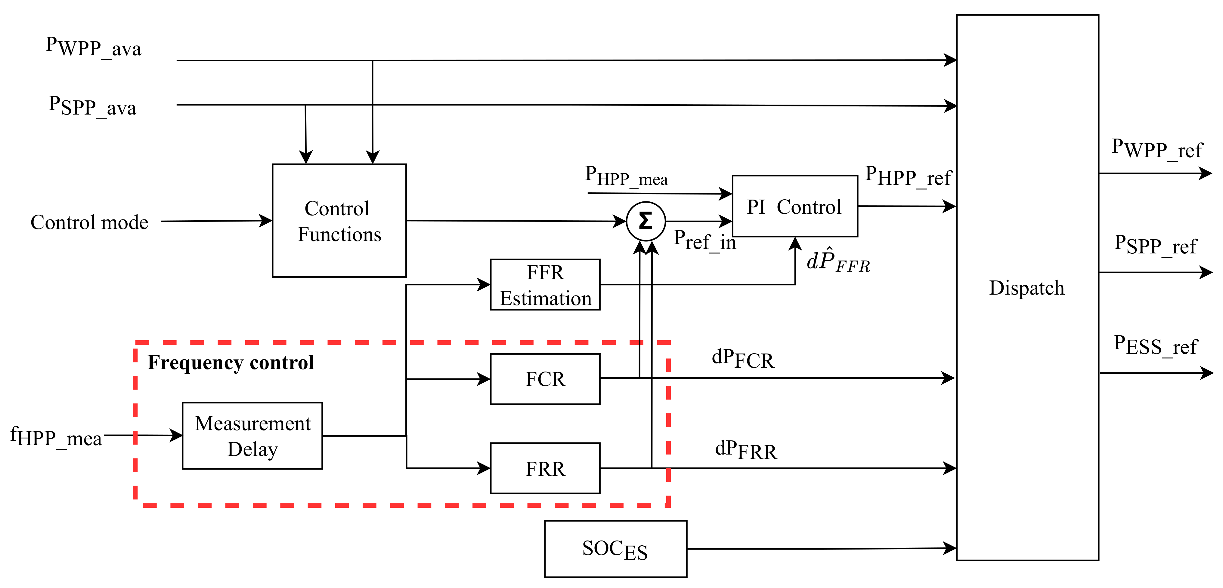
Figure 2.
HWPP controller.
Figure 2.
HWPP controller.
Figure 3.
WT model with integration of SC. (a) WT model integrating SC via a DC-DC converter. (b) WT model directly
integrating SC into DC link.
Figure 3.
WT model with integration of SC. (a) WT model integrating SC via a DC-DC converter. (b) WT model directly
integrating SC into DC link.
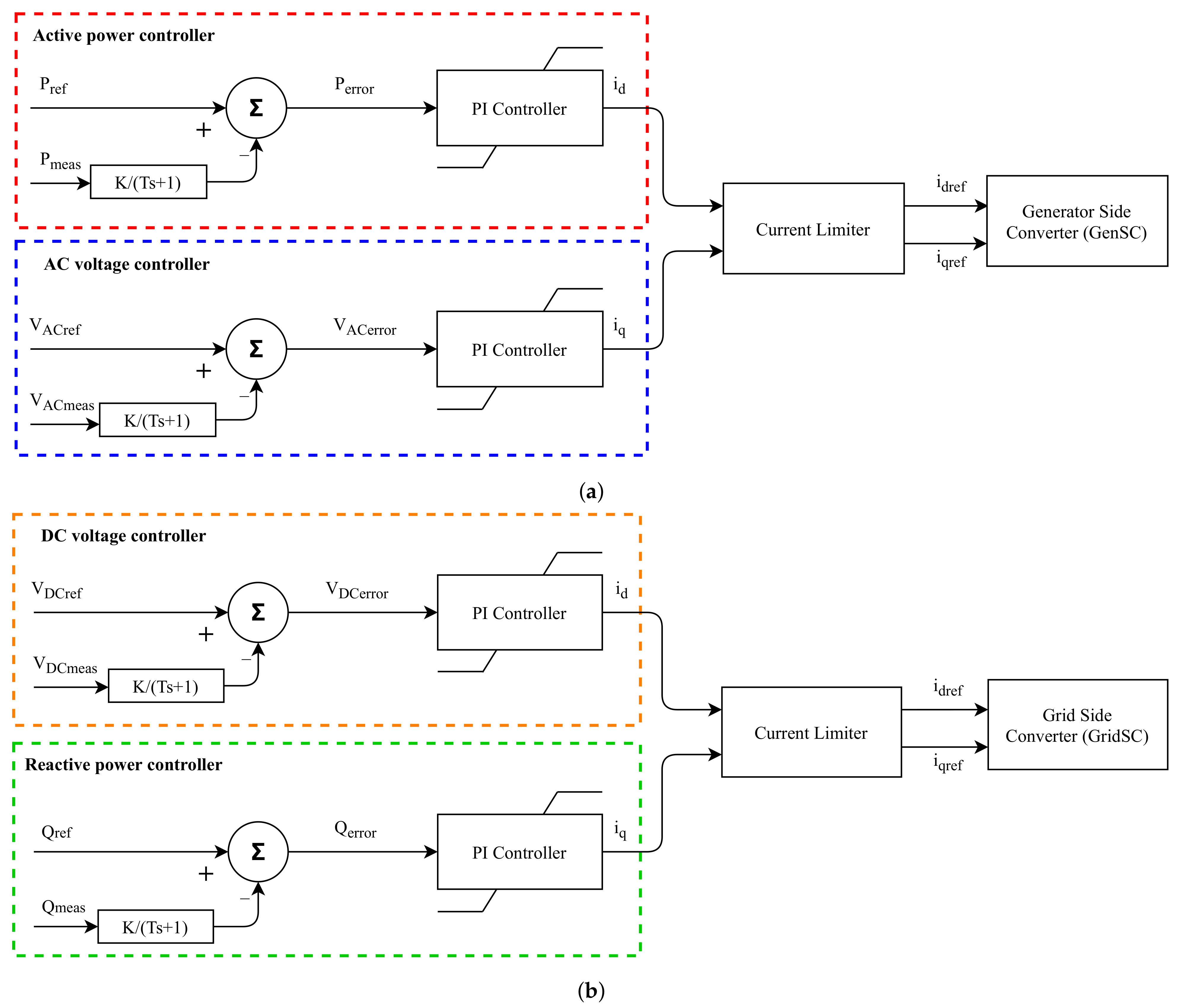
Figure 4.
WT converter controllers. (a) WT generator side converter controller. (b) WT grid side converter controller.
Figure 4.
WT converter controllers. (a) WT generator side converter controller. (b) WT grid side converter controller.
Figure 5.
SC controllers. (a) Controller for directly-connected SC. (b) Controller for converter-connected SC.
Figure 5.
SC controllers. (a) Controller for directly-connected SC. (b) Controller for converter-connected SC.
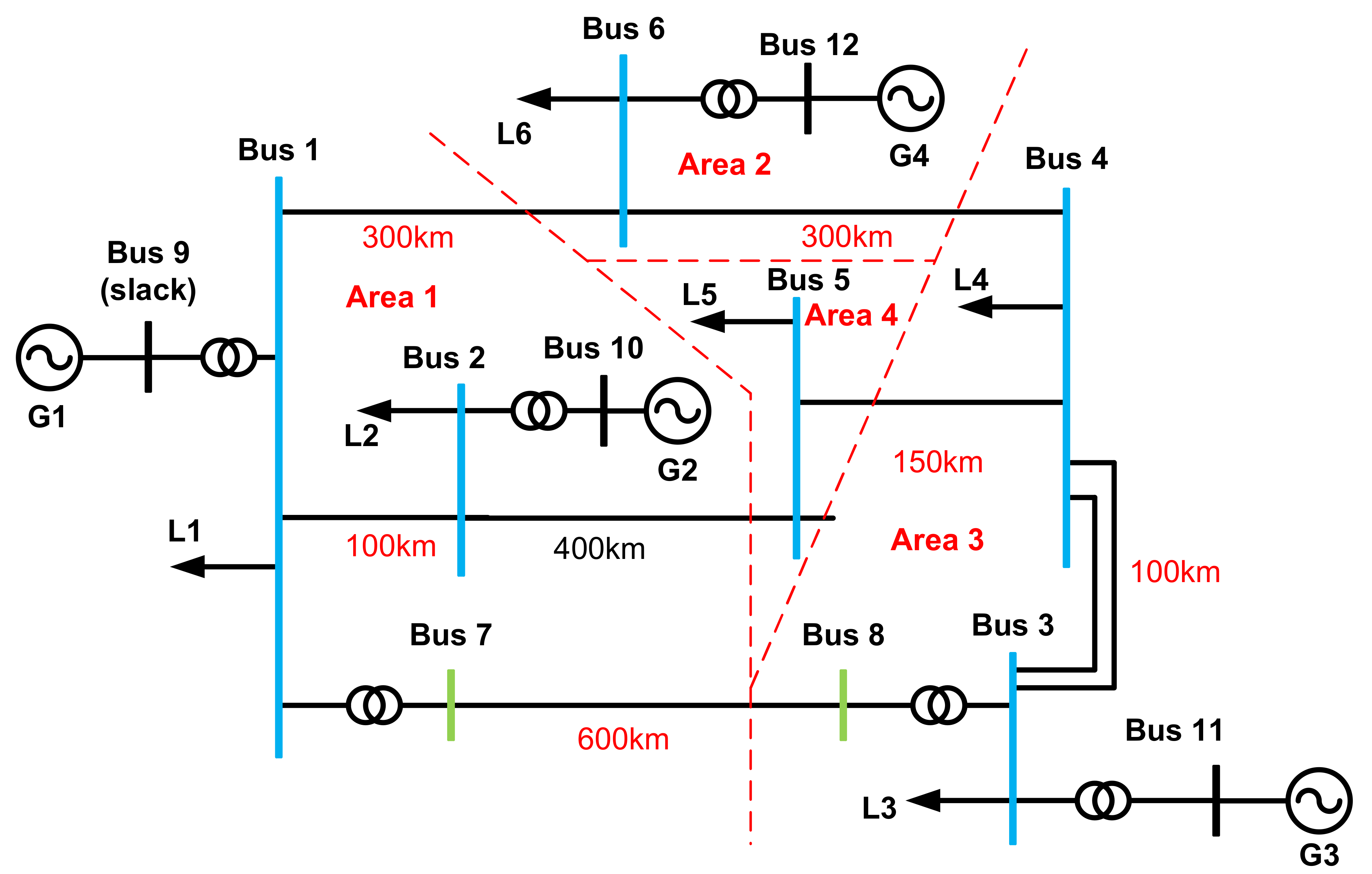
Figure 6.
Generic 12-bus system topology [
19].
Figure 6.
Generic 12-bus system topology [
19].
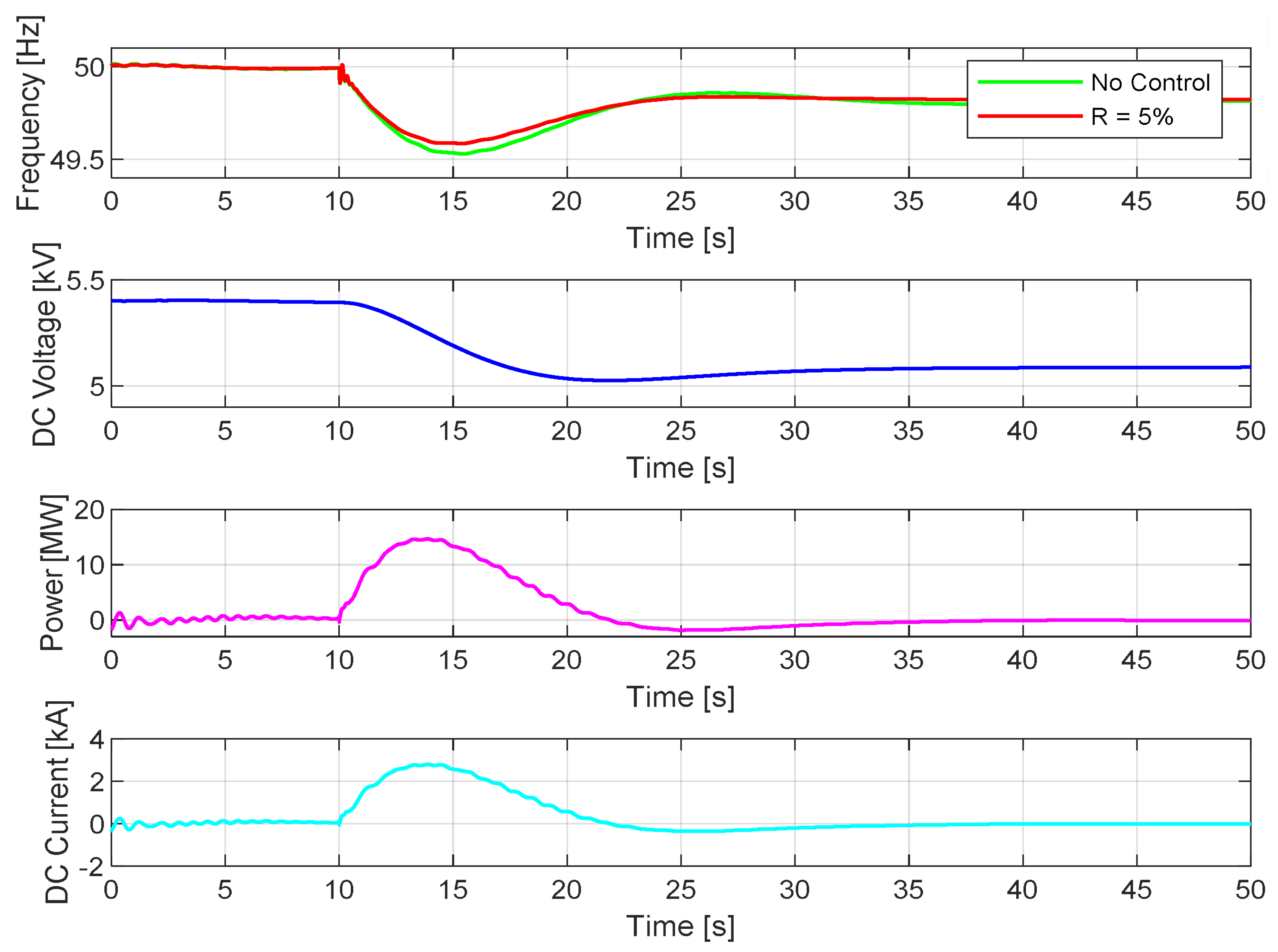
Figure 7.
FFR provision from the directly-connected SC (from top to bottom: system frequency, SC terminal DC voltage, SC output DC power, SC output DC current).
Figure 7.
FFR provision from the directly-connected SC (from top to bottom: system frequency, SC terminal DC voltage, SC output DC power, SC output DC current).
Figure 8.
FFR provision from the converter-connected SC (from top to bottom: system frequency, SC terminal DC voltage, SC output DC power, SC output DC current).
Figure 8.
FFR provision from the converter-connected SC (from top to bottom: system frequency, SC terminal DC voltage, SC output DC power, SC output DC current).
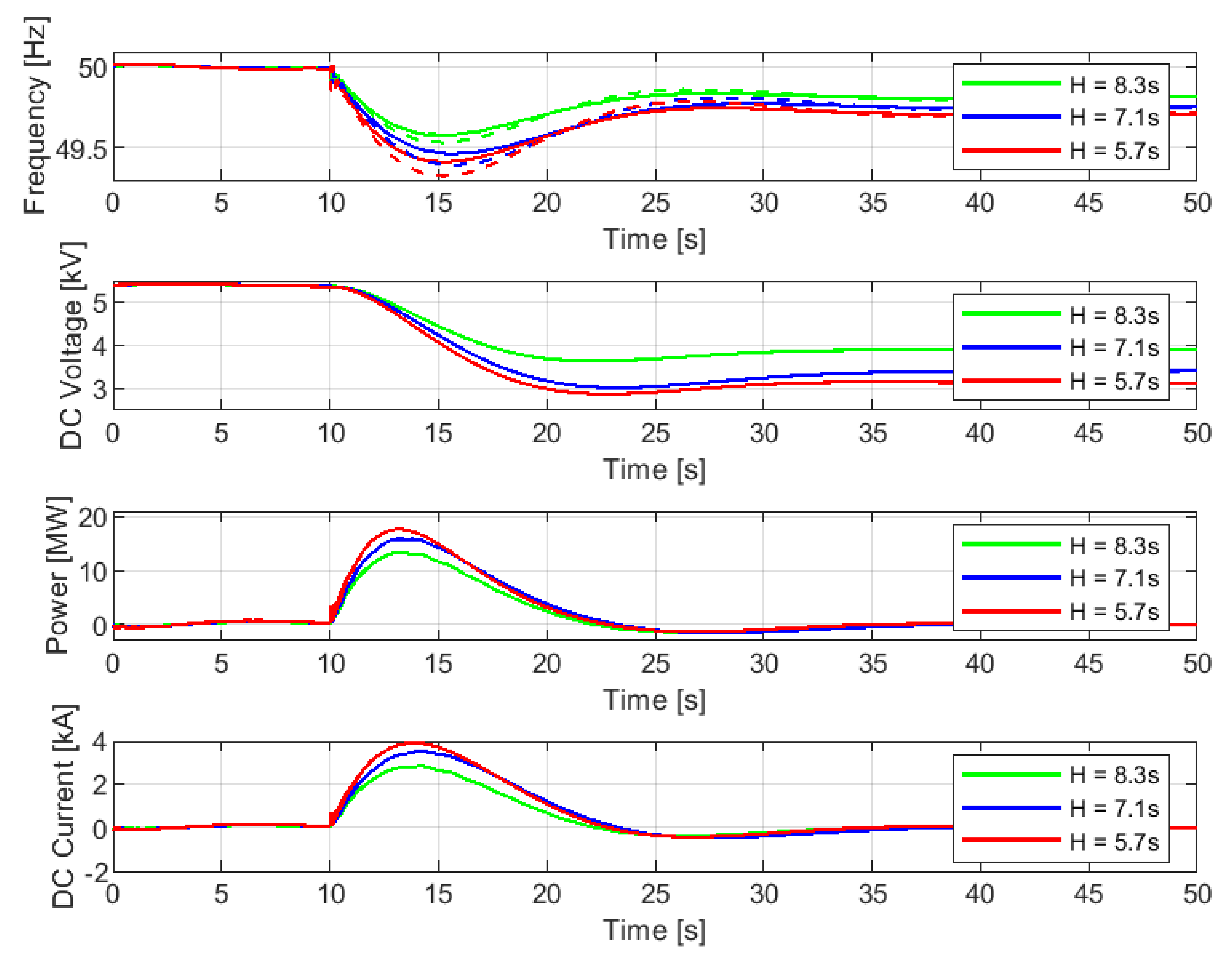
Figure 9.
FFR provision from the directly connected SC in systems with different inertia constants (from top to bottom: system frequency (solid lines—cases with control, dash lines—cases without control), SC terminal DC voltage, SC output DC power, SC output DC current).
Figure 9.
FFR provision from the directly connected SC in systems with different inertia constants (from top to bottom: system frequency (solid lines—cases with control, dash lines—cases without control), SC terminal DC voltage, SC output DC power, SC output DC current).
Figure 10.
FFR provision from the converter-connected SC in systems with different inertia constants: (from top to bottom: system frequency (solid lines—cases with control, dash lines—cases without control), SC terminal DC voltage, SC output DC power, SC output DC current).
Figure 10.
FFR provision from the converter-connected SC in systems with different inertia constants: (from top to bottom: system frequency (solid lines—cases with control, dash lines—cases without control), SC terminal DC voltage, SC output DC power, SC output DC current).
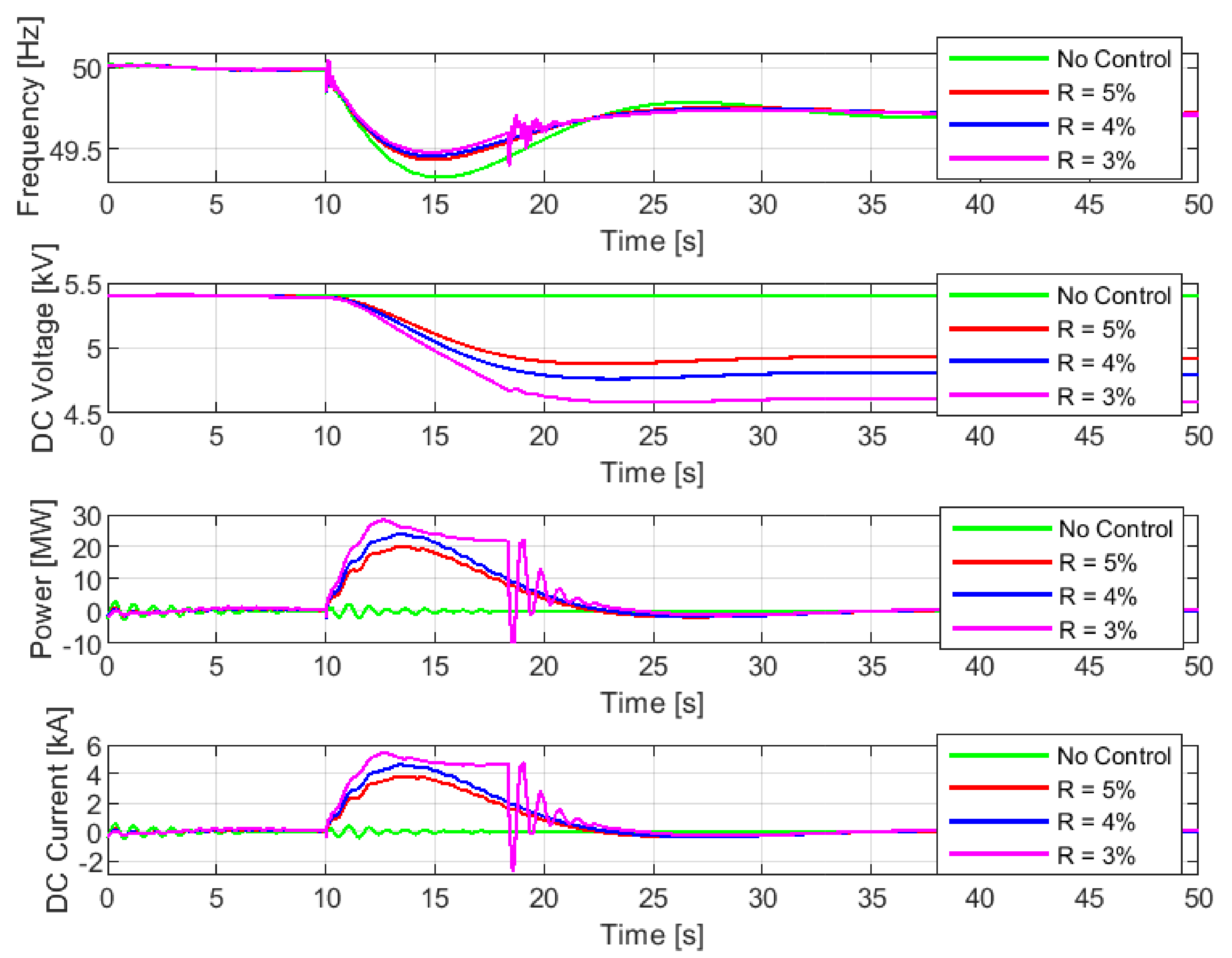
Figure 11.
FFR provision from the directly connected SC with varying droop coefficients (from top to bottom: system frequency, SC terminal DC voltage, SC output DC power, SC output DC current).
Figure 11.
FFR provision from the directly connected SC with varying droop coefficients (from top to bottom: system frequency, SC terminal DC voltage, SC output DC power, SC output DC current).
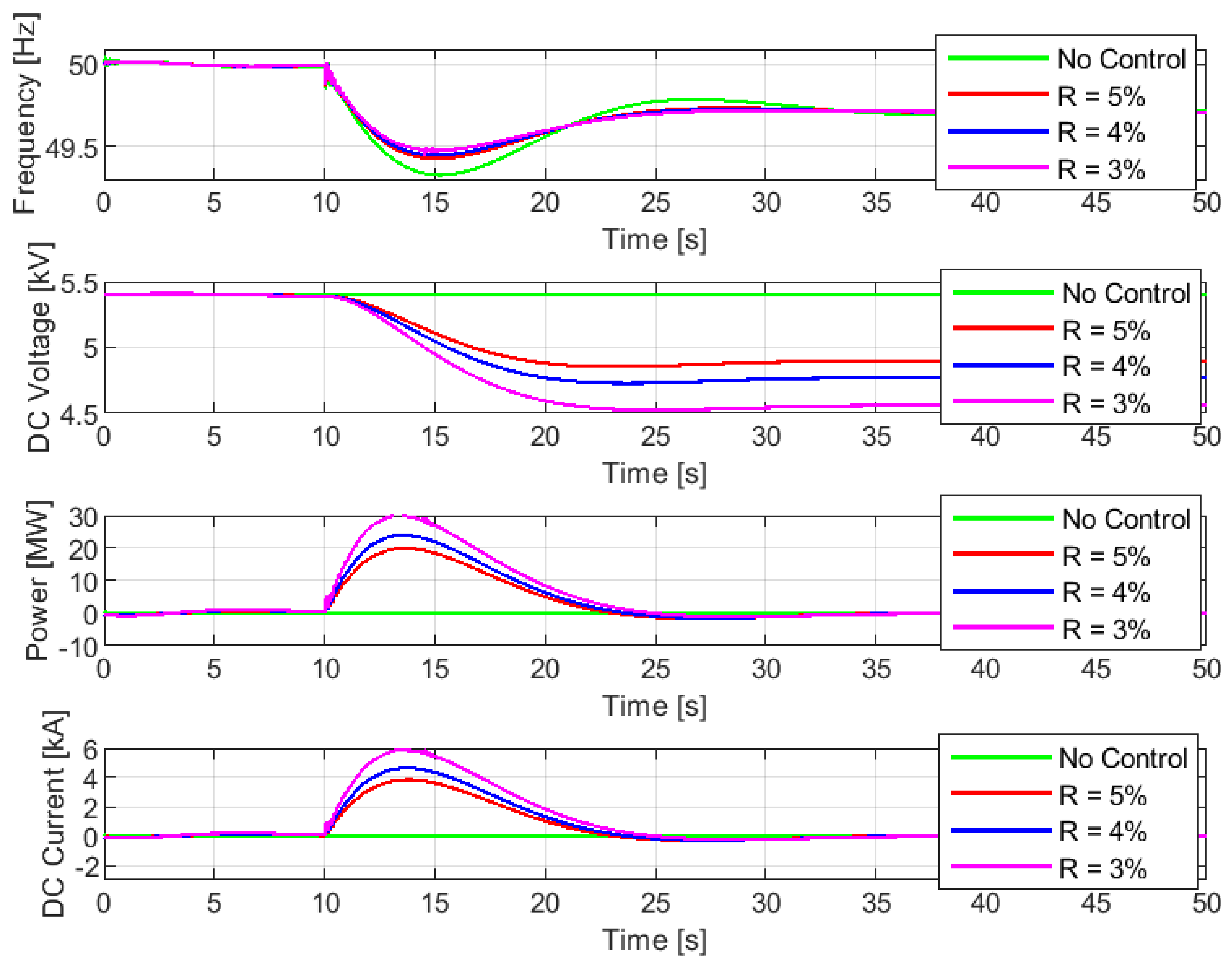
Figure 12.
FFR provision from the converter-connected SC with varying droop coefficients (from top to bottom: system frequency, SC terminal DC voltage, SC output DC power, SC output DC current).
Figure 12.
FFR provision from the converter-connected SC with varying droop coefficients (from top to bottom: system frequency, SC terminal DC voltage, SC output DC power, SC output DC current).
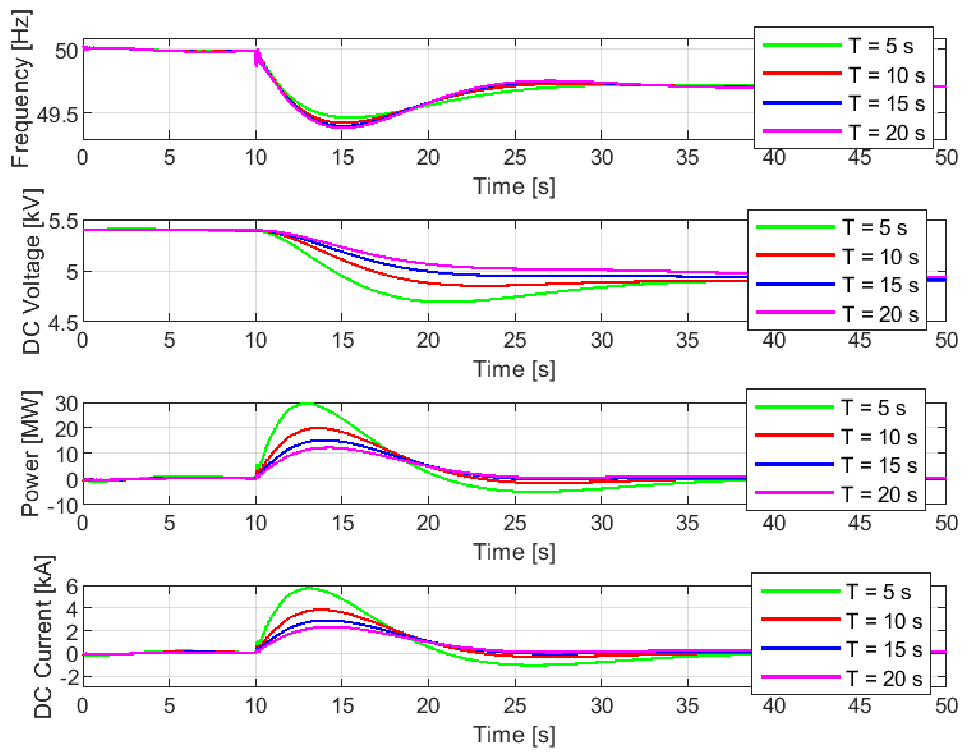
Figure 13.
FFR provision from the directly connected SC with varying time constants (from top to bottom: system frequency, SC terminal DC voltage, SC output DC power, SC output DC current).
Figure 13.
FFR provision from the directly connected SC with varying time constants (from top to bottom: system frequency, SC terminal DC voltage, SC output DC power, SC output DC current).
Figure 14.
FFR provision from the converter-connected SC with varying time constants (from top to bottom: system frequency, SC terminal DC voltage, SC output DC power, SC output DC current).
Figure 14.
FFR provision from the converter-connected SC with varying time constants (from top to bottom: system frequency, SC terminal DC voltage, SC output DC power, SC output DC current).
Table 1.
Overview of simulation results of FFR provision from the directly connected SC in systems with different inertia constants.
Table 1.
Overview of simulation results of FFR provision from the directly connected SC in systems with different inertia constants.
| Parameters | H = 8.3 s | H = 7.1 s | H = 5.7 s |
|---|
| Frequency Nadir Improvement (Hz) | | | |
| ROCOF Improvement (Hz/s) | | | |
| Minimum SC Voltage (kV) | | | |
| Maximum SC Power (MW) | | | |
| Maximum SC Current (kA) | | | |
Table 2.
Overview of simulation results of FFR provision from the converter-connected SC in systems with different inertia constants.
Table 2.
Overview of simulation results of FFR provision from the converter-connected SC in systems with different inertia constants.
| Parameters | H = 8.3 s | H = 7.1 s | H = 5.7 s |
|---|
| Frequency Nadir Improvement (Hz) | | | |
| ROCOF Improvement (Hz/s) | | | |
| Minimum SC Voltage (kV) | | | |
| Maximum SC Power (MW) | | | |
| Maximum SC Current (kA) | | | |
Table 3.
Overview of simulation results of FFR provision from the directly-connected SC in systems with varying droop coefficients.
Table 3.
Overview of simulation results of FFR provision from the directly-connected SC in systems with varying droop coefficients.
| Parameters | | | |
|---|
| Frequency Nadir Improvement (Hz) | | | |
| ROCOF Improvement (Hz/s) | | | |
| Minimum SC Voltage (kV) | | | |
| Maximum SC Power (MW) | | | |
| Maximum SC Current (kA) | | | |
Table 4.
Overview of simulation results of FFR provision from the converter-connected SC in systems with varying droop coefficients.
Table 4.
Overview of simulation results of FFR provision from the converter-connected SC in systems with varying droop coefficients.
| Parameters | | | |
|---|
| Frequency Nadir Improvement (Hz) | | | |
| ROCOF Improvement (Hz/s) | | | |
| Minimum SC Voltage (kV) | | | |
| Maximum SC Power (MW) | | | |
| Maximum SC Current (kA) | | | |
Table 5.
Overview of simulation results of FFR provision from the directly connected SC in systems with varying time constants.
Table 5.
Overview of simulation results of FFR provision from the directly connected SC in systems with varying time constants.
| Parameters | = 5 s | = 10 s | = 15 s | = 20 s |
|---|
| Frequency Nadir Improvement (Hz) | | | | |
| ROCOF Improvement (Hz/s) | | | | |
| Minimum SC Voltage (kV) | | | | |
| Maximum SC Power (MW) | | | | |
| Maximum SC Current (kA) | | | | |
Table 6.
Overview of simulation results of FFR provision from the converter-connected SC in systems with varying time constants.
Table 6.
Overview of simulation results of FFR provision from the converter-connected SC in systems with varying time constants.
| Parameters | = 5 s | = 10 s | = 15 s | = 20 s |
|---|
| Frequency Nadir Improvement (Hz) | | | | |
| ROCOF Improvement (Hz/s) | | | | |
| Minimum SC Voltage (kV) | | | | |
| Maximum SC Power (MW) | | | | |
| Maximum SC Current (kA) | | | | |


