
Finite Physical Dimensions Thermodynamics Analysis and Design of Closed Irreversible Cycles


Abstract
1. Introduction
- Stating the complete reversible trigeneration cycles for the fundamental energy schemes of providing imposed useful cooling, heating and power. This design level is very easily well done by considering ideal Carnot engine and refrigeration cycles. The ideal trigeneration built with completely ideal Carnot cycles gives the specific maximum maximorum energy efficiency, not depending on the working fluids’ nature, depending only on the external heat reservoirs temperatures related to the ideal Carnot engine cycle and to the ideal Carnot refrigeration cycle. These maximum maximorum energy efficiencies could be used for all kinds of assessments regarding the lost energy/exergy/irreversible entropy minimization.
- Defining the general endoreversible trigeneration thermodynamic models for all possible patterns of providing useful energies. This design level might be well completed through FPDT (finite physical dimensions thermodynamics) mathematical models based on the endoreversible Carnot cycles, see [14]. The limits of endoreversible Carnot cycles are surpassed through the mean thermodynamic temperature concept. However, it is obvious that the actual mean thermodynamic temperature is depending on the working fluids nature—i.e., on the thermodynamic properties—and on the type of the specific non adiabatic process. The FPDT (finite physical dimensions thermodynamics) mathematical models are general ones. The applications have to choose the working fluids and therefore the optimization might find the best working/convenient fluid by imposing simple or complex optimization criteria. The best actual FPDT endoreversible trigeneration becomes the reference case for all irreversible trigeneration cycles having the same working pattern.
- Defining the reference models assessing the irreversibility influence. The classical irreversibility analysis might be completed through thorough sensitivity analyses and specific optimization methods implying mean thermodynamic temperatures, specific lost exergy and irreversible entropy generation concepts. The FPDT assessments delineate a single concept evaluating priori the accumulated internal irreversibility, see for instance the short communications [15,16]. This evaluation of internal accumulated irreversibility by a single parameter is directly connecting the internal irreversibility to the external energy interactions through entropy balance equation. Therefore, through this single irreversibility dimensionless parameter the irreversible trigeneration assessments might be completed without knowing the working fluid nature and the type of thermal system. Although before each FPDT work they must be defined the operational possible domain range of this single parameter depending on the working fluid nature and on the thermal system type. They must also mention that the generalizing FPDT models of irreversible trigeneration have to adopt a new mean temperature of an external heat reservoir [14]. This new mean temperature is defined on the basis of the mean thermodynamic temperatures of the working fluid during the heat transfer processes and of the mean log temperature differences related to the linear heat transfer law. This new mean temperature can unify the first law and the linear heat transfer law without errors.
- Defining the design optimization approaches of reference reversible and irreversible cycles. The optimization procedures consider either pure thermodynamic criteria, or CAPEX criteria, or operational costs criteria, or environmental criteria. The more elaborated methods combine different criteria, e.g., multi-objective optimization.
- Defining the management optimization methods for possible interconnected trigeneration grids. They might be involved adaptive/intelligent management systems or trained predictive ones—e.g., training through fuzzy algorithms, management optimization methods such as MILP models, see reference [13].
2. The Irreversible Closed Cycles—The Irreversible Energy Efficiency—The Reference Entropy—The Number of Internal Irreversibility
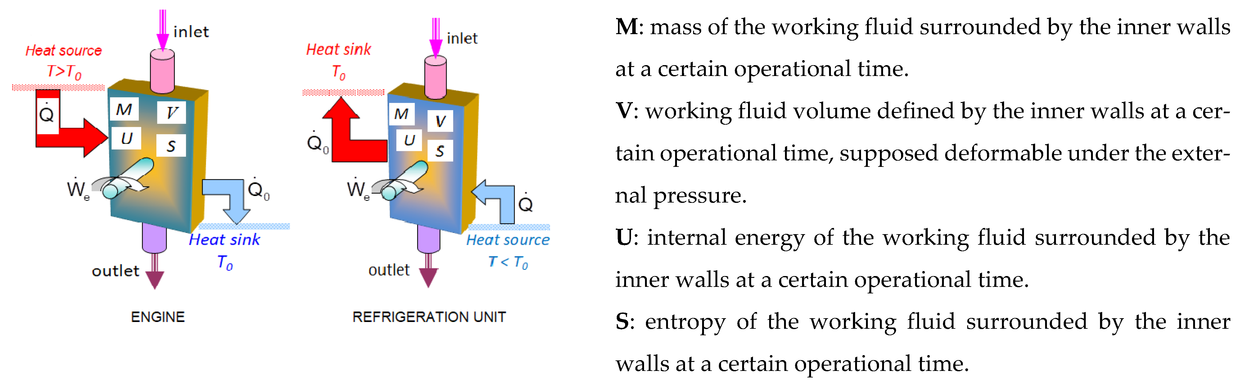
- the enlarged open thermal system comprising three interconnected parts and completely isolated from the universe, i.e., the proper open thermal system deformable under the external pressure which is joined with the external heat transfer reservoirs having known mean temperatures and heat capacities and joined with the deformation work and mass transfer reservoirs having known parameters, mass composition and specific energies (enthalpies, kinetic, and potential energies);
- the enlarged non-deformable closed thermal system that has two coupled parts isolated from the universe, the proper closed thermal system joined only with the external heat transfer reservoirs having known mean temperatures and specific heat capacities, and
- the closed thermal system/cycle considered alone but connected to external heat reservoirs with unknown parameters.
2.1. Assumptions for the First Case, the Enlarged Thermal Systems
- −
- They will be analyzed non steady-state enlarged basic open thermodynamic systems, including both the thermal system, and the external heat reservoirs controlling the heat transfers, and the environment allowing the mass transfers and the deformation work transfer under the external pressure, see Figure 1;
- −
- The working fluid is a mixture of different chemical species, the inlet and outlet compositions might be different because of chemical reactions that can appear during the flow through the thermal system, e.g., combustion;
- −
- The inner boundary of the flow path through the thermal system is deformable under the environmental pressure;
- −
- are the heat transfer rates from the heat source and to the heat sink, the real irreversible power, the complete reversible power and the lost power through irreversibility;
- −
- is the deformation work transfer under the external pressure, pe is the external pressure and V is the deformable volume of the thermal system;
- −
- , h, s are the mass flow rates, the specific enthalpy inclosing both the chemical and physical parts and the specific entropy inclosing both the chemical and physical parts, compulsory to obey to the first law of thermodynamics and considering all possible internal chemical processes, e.g., combustion;
- −
- are the specific kinetic and potential energies;
- −
- T, T0 are the mean temperatures of the heat source and of the heat sink;
- −
- is the entropy rate generated through whole irreversibility.
- −
- the reversible power transfer related to the reversible heat transfers, ideal Carnot cycle
- −
- the reversible power transfer caused by the reversible flow from the inlet states to outlet ones
- −
- the reversible power transfer related to the system reversible ‘energy inertia’ caused by non-steady state processes of the working fluid surrounded by the inner walls at a certain operational time
2.2. Assumptions Considering Closed Thermal Systems
- −
- no mass transfers
- −
- non deformable boundary walls, and
- −
- steady state operation
- −
- are the heat transfer rates;
- −
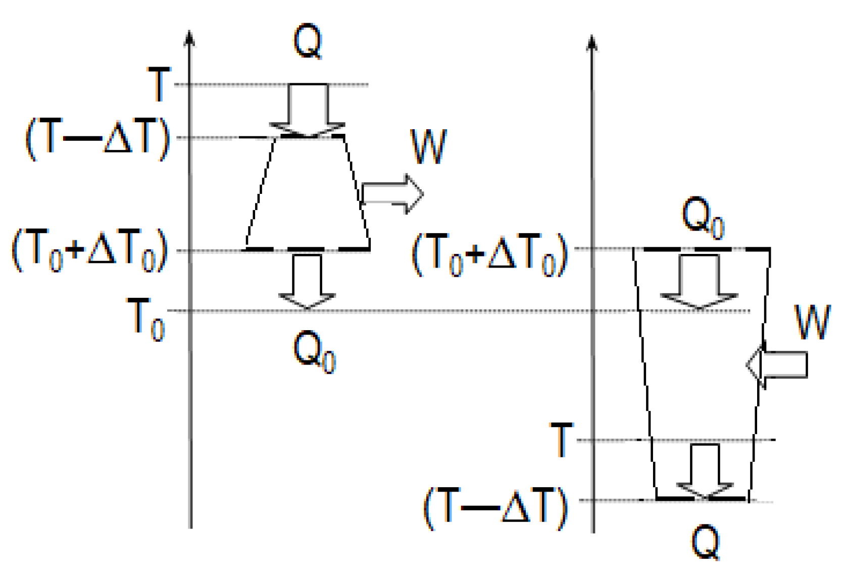
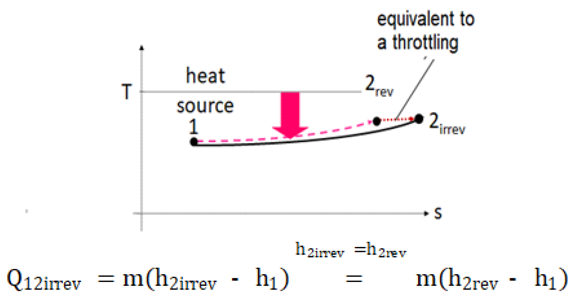
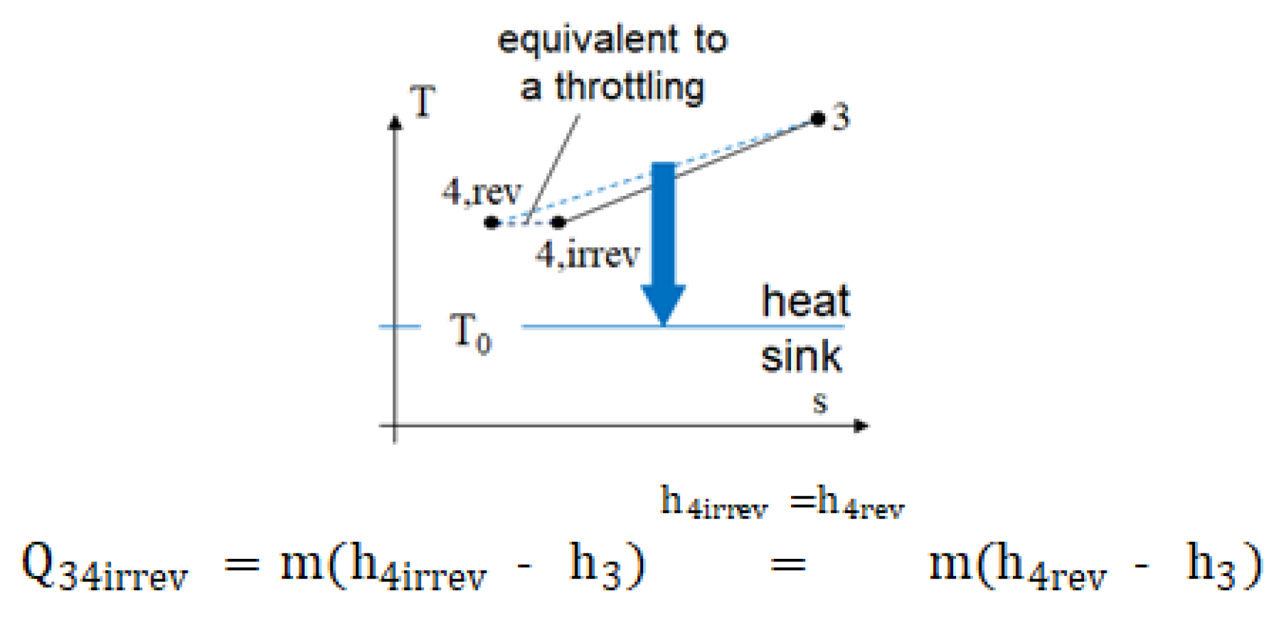
- are the mean temperatures of the heat source, of the heat sink and the corresponding mean log temperature differences controlling the heat transfers; they have to state that and are the mean thermodynamic temperatures of the working fluid for the reversible non adiabatic processes of the cycle, i.e., the reversible heating and cooling processes;
- −
- Irr is the comprehensive dimensionless irreversibility function linking the heat transfers through the entropy balance equation for the enlarged thermal system, it includes both the external irreversibility and the internal one;
- −
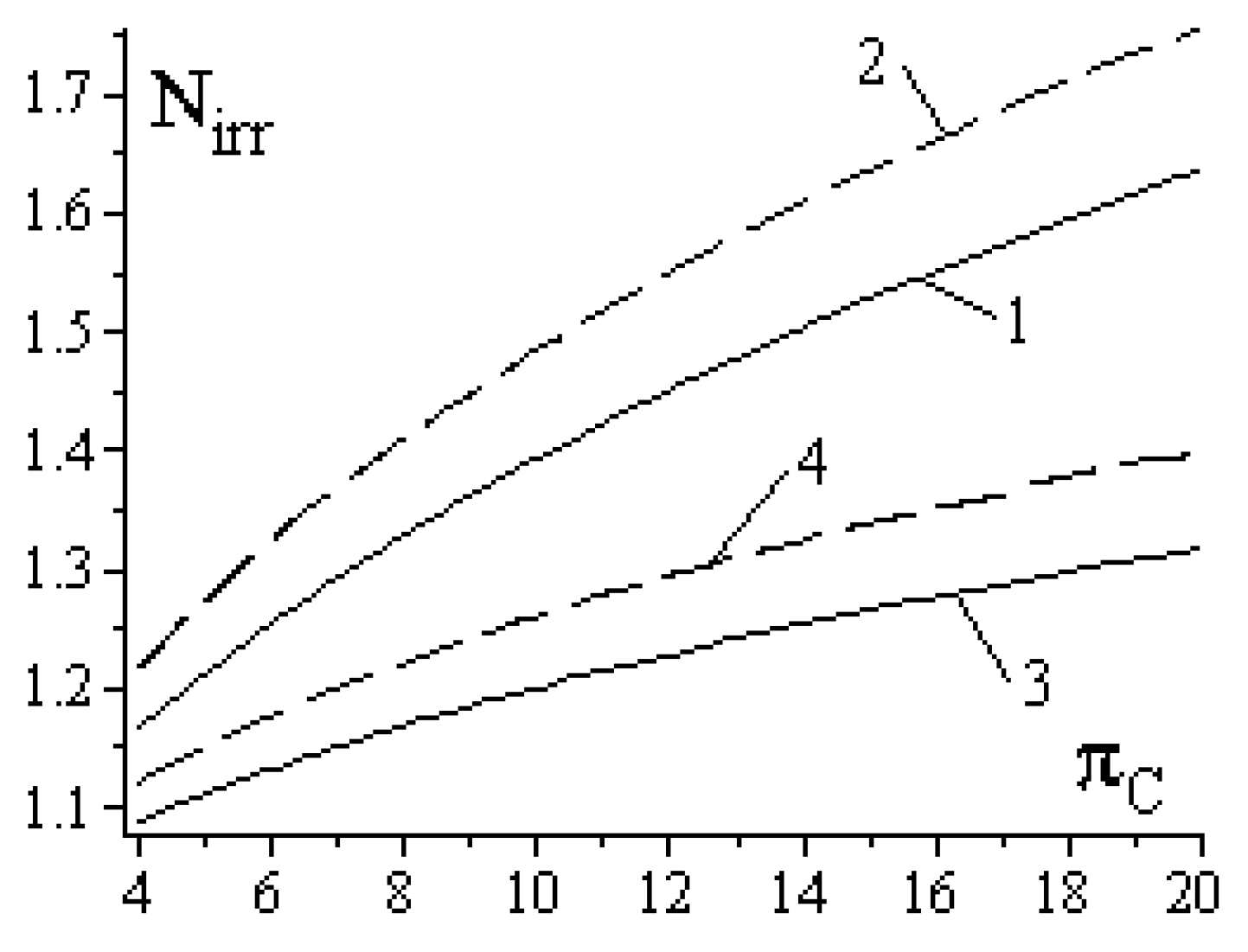
- Nirr is the internal dimensionless irreversibility function linking the heat transfers through entropy balance equation only for the thermal system, it includes only the internal irreversibility; in this paper Nirr is called as the number of internal irreversibility;
- −
- θHR, θmtt are the ratios of mean temperatures of external heat reservoirs and of mean thermodynamic temperatures of cycle’s non-adiabatic processes.
2.3. Irreversible Energy Efficiency of Enlarged Closed Thermal System
- Engine
- Refrigeration unit
2.4. Irreversible Energy Efficiency Only for the Closed Thermal System
- Engine
- Refrigeration unit
3. Design Imposed Operational Conditions
3.1. FPDT Internal Design through Imposed Operational Conditions
4. Irreversible Trigeneration Cycles External Design Based on FPDT
- engine cycle working in power mode and the reverse cycle working in refrigeration mode, the summer season;
- engine cycle working in cogeneration mode and the reverse cycle working in refrigeration mode, the winter season;
- engine cycle working in power mode and the reverse cycle working both in refrigeration mode and heat pump mode, the winter season; and
- engine cycle working in cogeneration mode and the reverse cycle working both in refrigeration mode and heat pump mode, the winter season.
4.1. Basic Mathematical Model
4.1.1. Engine Irreversible Cycle
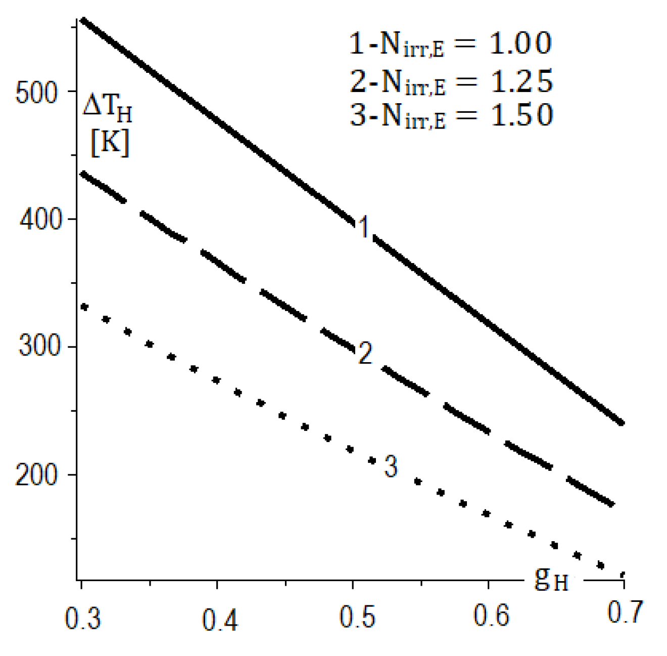
- Mean log temperature differences ΔTH [K] at the hot side and ΔTC [K] at the cold side.
- Thermal conductance [kW/K] allocated to the hot side, and thermal conductance [kW/K] allocated to the cold side.
- Thermal conductance inventory:
- −
- [kg·s−1] is the mass flow rate through engine;
- −
- [kW] is the reversible heat input rate;
- −
- [kW] is the reversible heat output rate;
- −
- [kW] is the power;
- −
- EEirr,E is the irreversible energy efficiency;
- −
- TH [K] is the mean thermodynamic temperature, cycle hot side;
- −
- [K] is the heat source proper mean temperature;
- −
- TC [K] is the mean thermodynamic temperature, cycle cold side;
- −
- [K] is the heat sink proper mean temperature;
4.1.2. Refrigeration Irreversible Cycle
- The reference entropy variation rate is:
- The finite physical dimension control parameters are: mean log temperature differences ΔTR [K] and ΔT0 [K], inside of heat exchangers at the heat source and at the heat sink;
- Thermal conductances inside the heat exchanger at the heat source, and inside the heat exchanger at the heat sink:
- First law balance equations:
- −
- [kg·s−1] is the mass flow rate of the working fluid through the refrigeration machine;
- −
- [kW] is the refrigeration heat rate;
- −
- [kW] is the heat rate at the heat sink;
- −
- [kW] is the consumed power
- −
- [K] is the mean thermodynamic temperature at the cycle cold side;
- −
- [K] is the mean temperature of the heat source;
- −
- T0 [K] is mean thermodynamic temperature at the cycle hot part;
- −
- is the mean temperature of the heat sink.
4.2. Irreversible Trigeneration System
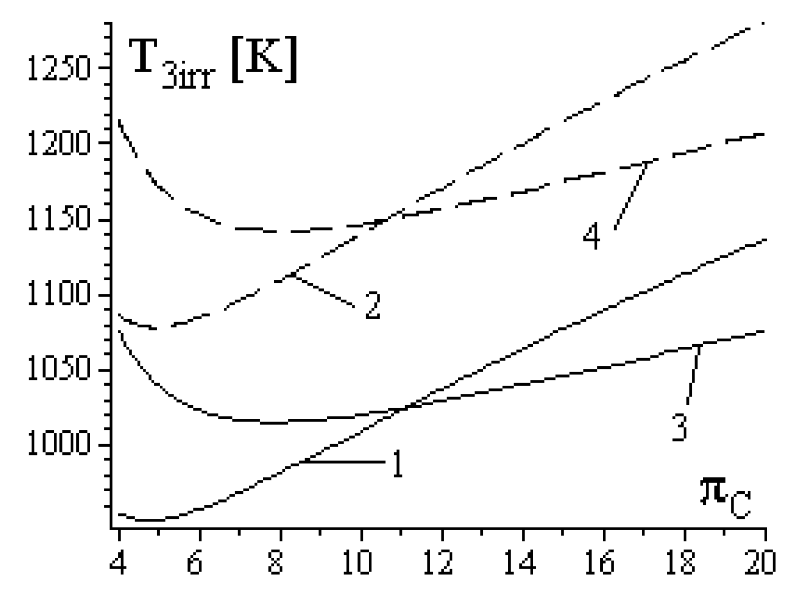
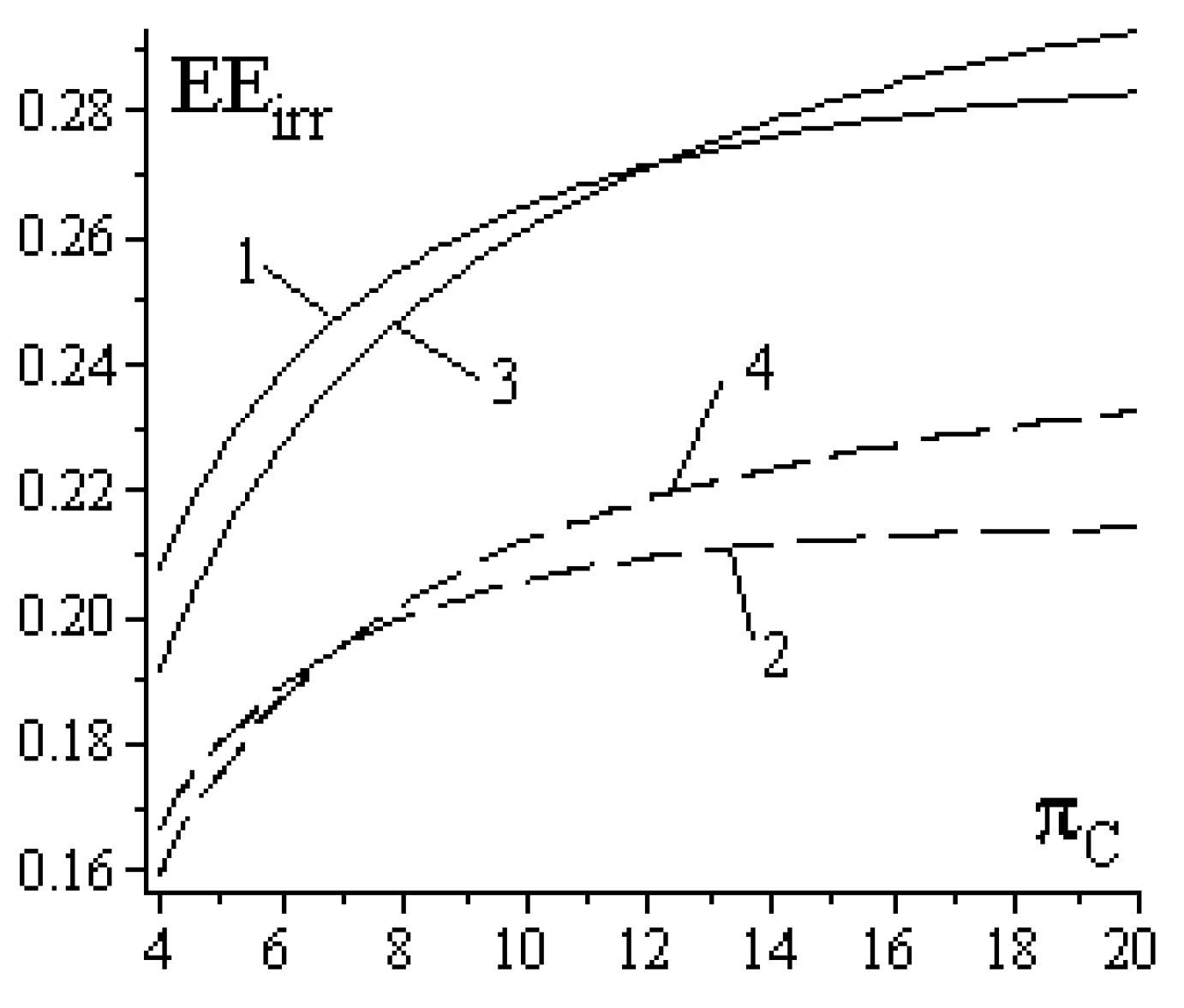
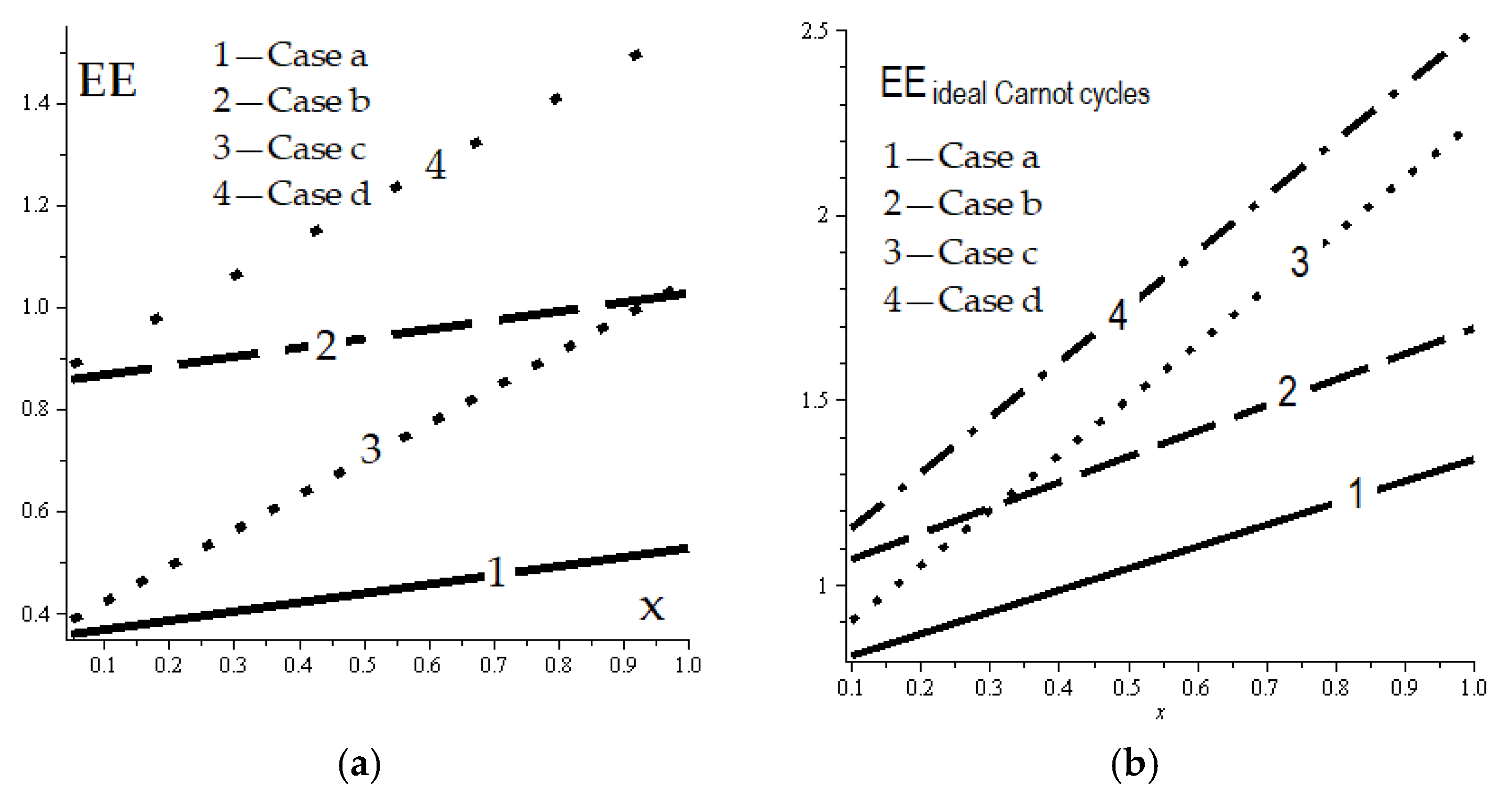
- Case “a”—energy efficiency:
- Case “b”—energy efficiency:
- Case “c”—energy efficiency:
- Case “d”—energy efficiency:
5. Conclusions
Author Contributions
Funding
Institutional Review Board Statement
Informed Consent Statement
Data Availability Statement
Acknowledgments
Conflicts of Interest
References
- Comodi, G.; Bartolini, A.; Carducci, F.; Nagaranjan, B.; Romagnoli, A. Achieving low carbon local energy communities in hot climates by exploiting networks synergies in multi energy systems. Appl. Energy 2019, 256, 113901. [Google Scholar] [CrossRef]
- Zhang, H.; Wang, L.; Lin, X.; Chen, H. Combined cooling, heating, and power generation performance of pumped thermal electricity storage system based on Brayton cycle. Appl. Energy 2020, 278, 115607. [Google Scholar] [CrossRef]
- Roy, D.; Samanta, S. Development and multiobjective optimization of a novel trigeneration system based on biomass energy. Energy Convers. Manag. 2021, 240, 114248. [Google Scholar] [CrossRef]
- Villarini, M.; Tascioni, R.; Arteconi, A.; Cioccolanti, L. Influence of the incident radiation on the energy performance of two small-scale solar organic Rankine cycle trigenerative systems: A simulation analysis. Appl. Energy 2019, 242, 1176–1188. [Google Scholar] [CrossRef]
- Sameti, M.; Haghighat, F. Integration of distributed energy storage into net-zero energy district systems: Optimum design and operation. Energy 2018, 153, 575–591. [Google Scholar] [CrossRef]
- Huang, Y.; Wang, Y.; Chen, H.; Zhang, X.; Mondol, J.; Shah, N.; Hewitt, N. Performance analysis of biofuel fired trigeneration systems with energy storage for remote households. Appl. Energy 2017, 186, 530–538. [Google Scholar] [CrossRef]
- Kasaeian, A.; Bellos, E.; Shamaeizadeh, A.; Tzivanidis, C. Solar-driven polygeneration systems: Recent progress and outlook. Appl. Energy 2020, 264, 114764. [Google Scholar] [CrossRef]
- Braun, R.; Haag, M.; Stave, J.; Abdelnour, N.; Eicker, U. System design and feasibility of trigeneration systems with hybrid photovoltaic-thermal (PVT) collectors for zero energy office buildings in different climates. Sol. Energy 2020, 196, 39–48. [Google Scholar] [CrossRef]
- Urbanucci, L.; Bruno, J.C.; Testi, D. Thermodynamic and economic analysis of the integration of high-temperature heat pumps in trigeneration systems. Appl. Energy 2019, 238, 516–533. [Google Scholar] [CrossRef]
- Marques, A.S.; Carvalho, M.; Ochoa, A.A.; Abrahão, R.; Santos, C.A. Life cycle assessment and comparative exergoenvironmental evaluation of a micro-trigeneration system. Energy 2021, 216, 119310. [Google Scholar] [CrossRef]
- Sztekler, K.; Kalawa, W.; Mika, L.; Krzywanski, J.; Grabowska, K.; Sosnowski, M.; Nowak, W.; Siwek, T.; Bieniek, A. Modeling of a Combined Cycle Gas Turbine Integrated with an Adsorption Chiller. Energies 2020, 13, 515. [Google Scholar] [CrossRef]
- Villarroel-Schneider, J.; Malmquist, A.; Araoz, J.A.; Martí-Herrero, J.; Martin, A. Performance Analysis of a Small-Scale Bio-gas-Based Trigeneration Plant: An Absorption Refrigeration System Integrated to an Externally Fired Microturbine. Energies 2019, 12, 3830. [Google Scholar] [CrossRef]
- Bischi, A.; Taccari, L.; Martelli, E.; Amaldi, E.; Manzolini, G.; Silva, P.; Campanari, S.; Macchi, E. A detailed MILP optimization model for combined cooling, heat and power system operation planning. Energy 2014, 74, 12–26. [Google Scholar] [CrossRef]
- Gheorghe, D.; Michel, F.; Aristotel, P.; Stefan, G. Endoreversible trigeneration cycle design based on finite physical dimensions thermodynamics. Energies 2019, 12, 3165. [Google Scholar] [CrossRef]
- Dumitrascu, G. The way to optimize the irreversible cycles. Termotehnica 2008, 2, 18–21. [Google Scholar]
- Dumitrascu, G.; Feidt, M.; Grigorean, S. Closed Irreversible Cycles Analysis Based on Finite Physical Di-mensions Thermodynamics. In Proceedings of the First World Energies Forum, Rome, Italy, 4 September–5 October 2020; Available online: https://wef.sciforum.net/ (accessed on 11 September 2020).
- Kestin, J. A Course in Thermodynamics; Hemisphere: Washington, DC, USA, 1979; Volume 1, pp. 40, 223. [Google Scholar]
- Bejan, A. Advanced Engineering Thermodynamics, 3rd ed.; Wiley: Hoboken, NJ, USA, 2006; p. 22. [Google Scholar]
- Dumitrașcu, G.; Feidt, M.; Namat, A.R.J.; Grigorean, Ş.; Horbaniuc, B. Thermodynamic analysis of irreversible closed Brayton engine cycles used in trigeneration systems. In IOP Conference Series: Materials Science and Engineering, Proceedings of the The XXIInd National Conference on Thermodynamics with International Participation, Galati, Romania, 23–24 May 2019; IOP Publishing Ltd.: Bristol, UK, 2019; Volume 595, p. 012022. [Google Scholar] [CrossRef]


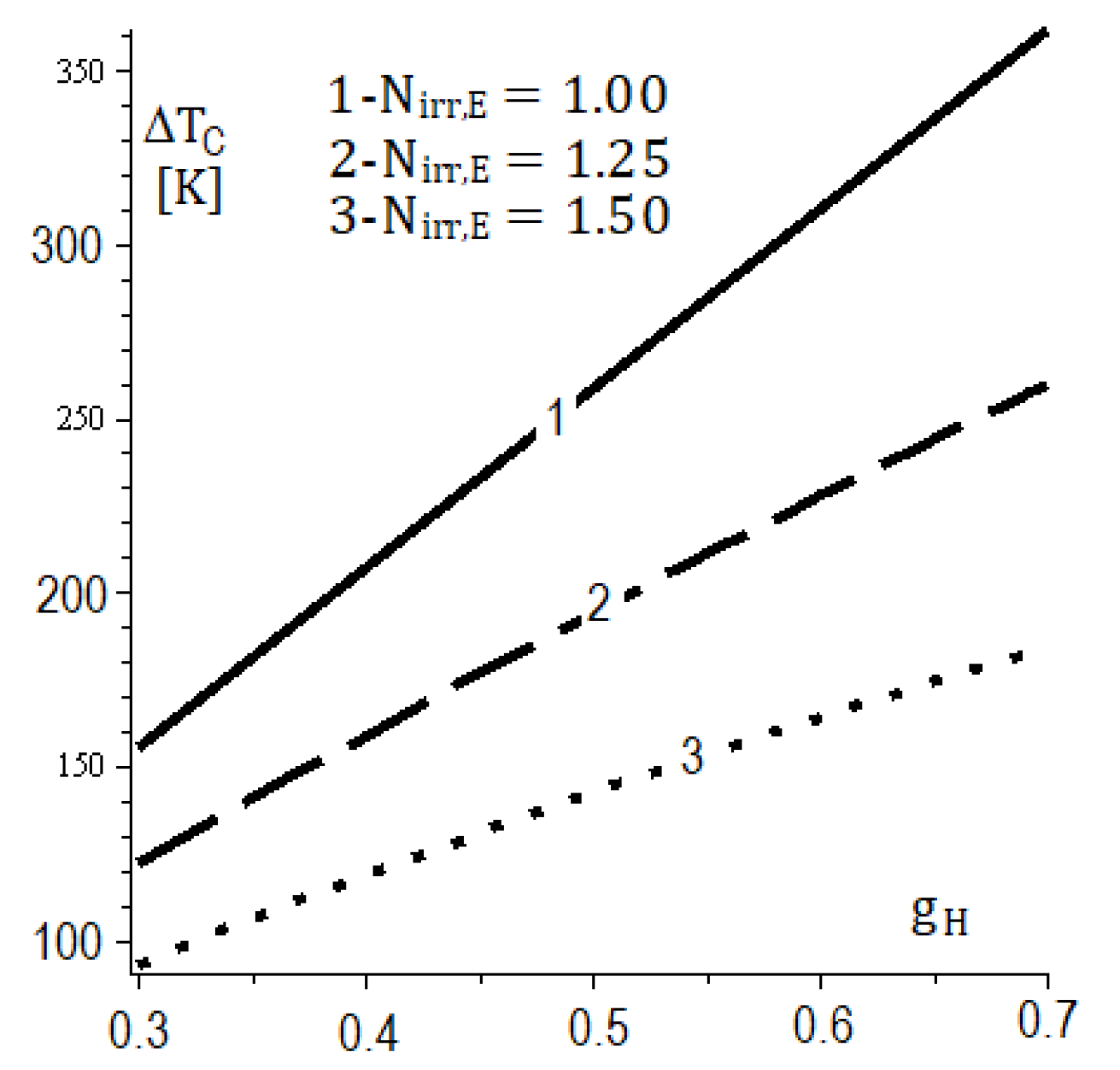
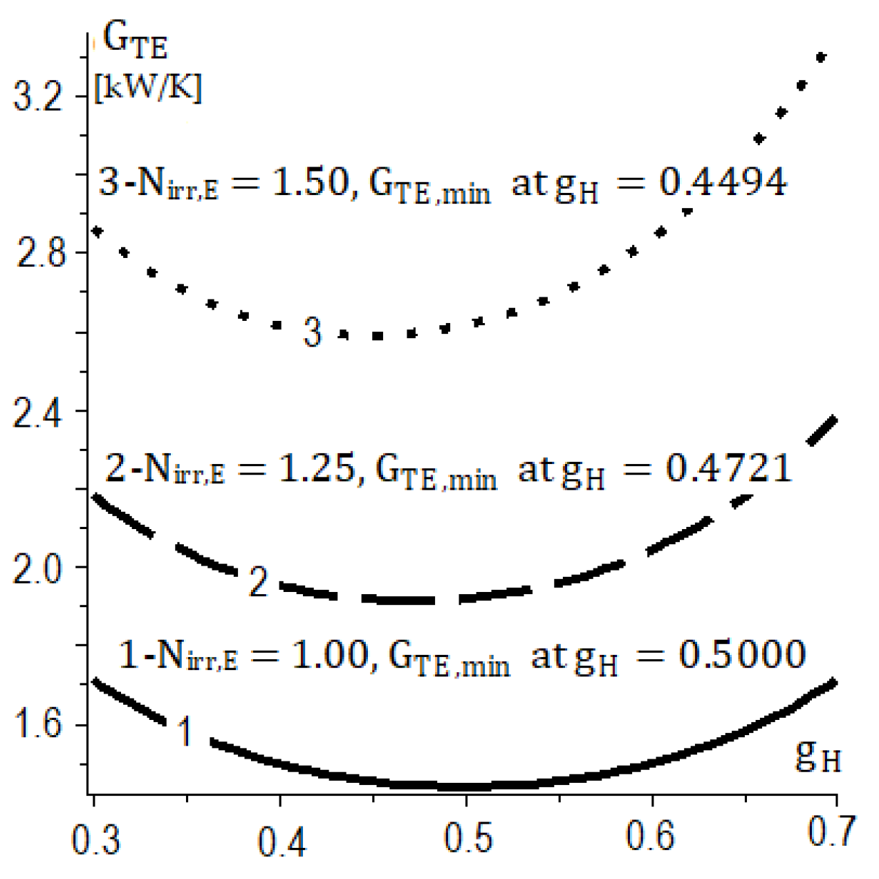
| Trigeneration | Nirr | TCS (K) | ΔTH (K) | ΔTC (K) | GTE (kW·K−1) | |
|---|---|---|---|---|---|---|
| (a) | 1.00 | 0.5000 | 308 | 379 | 246 | 1.507 |
| 1.25 | 0.4721 | 308 | 302 | 176 | 2.003 | |
| 1.50 | 0.4494 | 308 | 234 | 124 | 2.713 | |
| (b) | 1.00 | 0.5000 | 343 | 422 | 274 | 1.354 |
| 1.25 | 0.4721 | 343 | 336 | 196 | 1.799 | |
| 1.50 | 0.4494 | 343 | 261 | 138 | 2.436 | |
| (c) | 1.00 | 0.5000 | 273 | 336 | 218 | 1.701 |
| 1.25 | 0.4721 | 273 | 268 | 156 | 2.261 | |
| 1.50 | 0.4494 | 273 | 208 | 110 | 3.061 | |
| (d) | 1.00 | 0.5000 | 343 | 422 | 274 | 1.354 |
| 1.25 | 0.4721 | 343 | 336 | 196 | 1.799 | |
| 1.50 | 0.4494 | 343 | 261 | 138 | 2.436 |
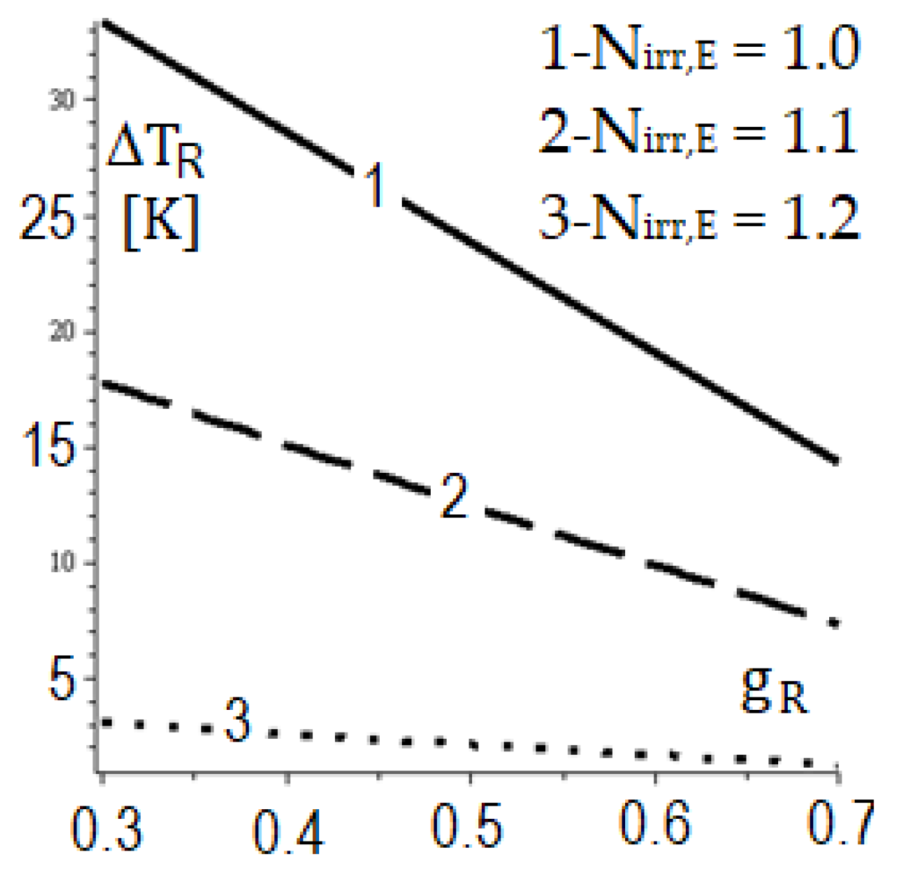
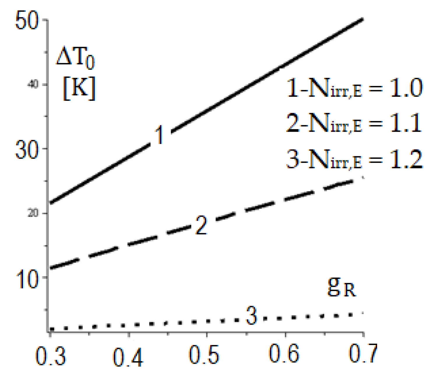
| Trigeneration | Nirr | T0S (K) | TRS (K) | ΔTR (K) | ΔT0 (K) | GTR (kW·K−1) | COP | |
|---|---|---|---|---|---|---|---|---|
| (a) | 1.0 | 0.500 | 308 | 253 | 23.83 | 35.75 | 0.839 | 2 |
| 1.1 | 0.488 | 308 | 253 | 13.24 | 18.83 | 1.547 | 2 | |
| 1.2 | 0.477 | 308 | 253 | 3.15 | 4.31 | 6.503 | 2 | |
| (b) | 1.0 | 0.500 | 273 | 253 | 24.13 | 32.17 | 0.829 | 3 |
| 1.1 | 0.488 | 273 | 253 | 13.56 | 17.13 | 1.511 | 3 | |
| 1.2 | 0.477 | 273 | 253 | 3.49 | 4.24 | 5.88 | 3 | |
| (c) | 1.0 | 0.500 | 343 | 253 | 23.60 | 39.33 | 0.875 | 1.5 |
| 1.1 | 0.488 | 343 | 253 | 13.00 | 20.53 | 1.577 | 1.5 | |
| 1.2 | 0.477 | 343 | 253 | 2.88 | 4.38 | 7.106 | 1.5 | |
| (d) | 1.0 | 0.500 | 343 | 253 | 23.60 | 39.33 | 0.875 | 1.5 |
| 1.1 | 0.488 | 343 | 253 | 13.00 | 20.53 | 1.577 | 1.5 | |
| 1.2 | 0.477 | 343 | 253 | 2.88 | 4.38 | 7.106 | 1.5 |
Publisher’s Note: MDPI stays neutral with regard to jurisdictional claims in published maps and institutional affiliations. |
© 2021 by the authors. Licensee MDPI, Basel, Switzerland. This article is an open access article distributed under the terms and conditions of the Creative Commons Attribution (CC BY) license (https://creativecommons.org/licenses/by/4.0/).
Share and Cite
Dumitrașcu, G.; Feidt, M.; Grigorean, Ş. Finite Physical Dimensions Thermodynamics Analysis and Design of Closed Irreversible Cycles. Energies 2021, 14, 3416. https://doi.org/10.3390/en14123416
Dumitrașcu G, Feidt M, Grigorean Ş. Finite Physical Dimensions Thermodynamics Analysis and Design of Closed Irreversible Cycles. Energies. 2021; 14(12):3416. https://doi.org/10.3390/en14123416
Chicago/Turabian StyleDumitrașcu, Gheorghe, Michel Feidt, and Ştefan Grigorean. 2021. "Finite Physical Dimensions Thermodynamics Analysis and Design of Closed Irreversible Cycles" Energies 14, no. 12: 3416. https://doi.org/10.3390/en14123416
APA StyleDumitrașcu, G., Feidt, M., & Grigorean, Ş. (2021). Finite Physical Dimensions Thermodynamics Analysis and Design of Closed Irreversible Cycles. Energies, 14(12), 3416. https://doi.org/10.3390/en14123416