A Practical GERI-Based Method for Identifying Multiple Erroneous Parameters and Measurements Simultaneously

Abstract

Even with modern smart metering systems, erroneous measurements of the real and reactive power in the power system are unavoidable. Multiple erroneous parameters and measurements may occur simultaneously in the state estimation of a bulk power system. This paper proposes a gross error reduction index (GERI)-based method as an additional module for existing state estimators in order to identify multiple erroneous parameters and measurements simultaneously. The measurements are acquired from a supervisory control and data acquisition system and mainly include voltage amplitudes, branch current amplitudes, active power flow, and reactive power flow. This method uses a structure consisting of nested two loops. First, gross errors and the GERI indexes are calculated in the inner loop. Second, the GERI indexes are compared and the maximum GERI in each inner loop is associated with the most suspicious parameter or measurement. Third, when the maximum GERI is less than a given threshold in the outer loop, its corresponding erroneous parameter or measurement is identified. Multiple measurement scans are also adopted in order to increase the redundancy of measurements and the observability of parameters. It should be noted that the proposed algorithm can be directly integrated into the Weighted Least Square estimator. Furthermore, using a faster simplified calculation technique with Givens rotations reduces the required computer memory and increases the computation speed. This method has been demonstrated in the IEEE 14-bus test system and several matpower cases. Due to its outstanding practical performance, it is now used at six provincial power control centers in the Eastern Grid of China.

1. Introduction

State estimation (SE) has a strong impact on power system applications in a smart grid [1]. Even with modern smart metering systems, erroneous measurements of the real and reactive power in the power system are unavoidable. Multiple erroneous parameters and measurements may occur simultaneously in the state estimation of a bulk power system.

Traditional detection methods for erroneous measurements assume that the values of the network parameters are precisely correct [2]. These methods detect and identify measurement errors effectively using residual analysis (sum of squared residuals [3] and weighted-normalized residuals [4,5]) and nonquadratic criteria [6]. However, one erroneous parameter, e.g., branch impedance, usually produces an obscure error. The parameter error and the set of correlated measurement errors on the same branch have the same effect on SE [7]. Thus, parameter errors are misidentified, negatively influencing the SE.

Parameter errors occur when data are entered incorrectly or fail to be updated in time, etc. [1,7]. Parameter identification and estimation are considered sequentially in traditional parameter estimation methods. These methods are typically performed using either residual sensitivity analysis [8,9,10] or augmented SE [11,12,13,14,15,16]. The first approach does not need to modify the core SE code and is, thus, easy to implement, as the sensitivities of measurement residuals to measurement errors can be directly acquired from solved SE cases. However, the identification results are easily corrupted by parameter and measurement errors. The second approach identifies parameter errors by treating suspicious parameters as additional state variables to estimate. Such calculations can be performed with static normal equations [11,12,13] or the Kalman filter theory [14,15,16]. Their advantages and disadvantages are shown in Reference [7].

The normalized Lagrange multipliers (NLM) method [17,18,19,20,21] uses measurement residuals to calculate the Lagrange multipliers of parameters. By comparing the normalized measurement residuals representing measurement errors and Lagrange multipliers representing parameter errors with a threshold, erroneous parameters and measurements can be identified simultaneously [18]. To increase the redundancy of measurements, researchers have adopted synchronized phasors [19] and multiple measurement scans [20,21].

The problem of parameter errors and measurement errors is usually studied using the least square method. Reference [22] proposes a phasor measurement unit-based positive sequence measurement error model to identify parameter errors based on the Weighted Least Square (WLS) SE. Reference [23] combines adaptive linear neuron and the traditional robust IGG method for parameter identification by training the adaptive linear neuron with the least mean square algorithm. Reference [24] adopts Gaussian least squares differential correction to identify the gross error between estimated values and measured data. Based on an intelligent measurement infrastructure, Reference [25] makes full use of the simplicity and accuracy of the improved nonlinear least square method to identify erroneous parameters.

Compared with the above algorithms, a robust state estimation directly eliminates the influence of parameter errors on SE without having to go through the steps of identifying, correcting, and removing erroneous parameters [26]. Reference [27] conducts a two-stage WLS SE to reduce the negative effect of measurement errors directly. Reference [28] calculates transmission line parameters at both ends of a line using median estimation to reduce the impact of measurement errors. Reference [29] automatically updates the weighting factors of measurement dependencies with a robust state estimation method based on the WLS SE model. Reference [30] uses the genetic learning particle swarm optimization hybrid algorithm for the robust state estimation method to estimate the key parameters. Seven robust methods for line impedance estimation using fast voltage and current variation measurement are compared in an analysis of real measured data [31]. However, the robust state estimation requires extreme changes to existing power system SE applications.

This paper proposes a gross error reduction index (GERI)-based method as an additional module for an existing state estimator to identify multiple erroneous parameters and measurements simultaneously.

In addition, identification methods adopt multiple measurement scans to increase the redundancy of measurements and the observability of parameters in References [10,16,20,21]. The GERI-based method also adopts multiple measurement scans in this paper.

In the bulk power system, the existence of erroneous parameters is harmful to SE. Moreover, we try to explore a parameter identification method applied easily in the bulk power system. The GERI-based method is adopted to simultaneously identify multiple erroneous parameters and measurements. Its contributions are as follows:

(1)

Identifying multiple erroneous parameters and measurements simultaneously with only one WLS SE.

(2)

Being an additional module integrated into the WLS state estimator with minor changes in the WLS SE code.

(3)

Adopting the simplified calculation of variables to increase the computation speed and reduce the required computer memory.

(4)

Adopting multiple measurement scans to increase the redundancy of measurements without any investment in new meters.

The rest of the paper is organized as follows. We derive the formulation of the GERI-based method in Section 2. In Section 3, a simplified calculation of variables is deduced and the different effects of multiple measurement scans on erroneous parameters and measurements are analyzed. In Section 4, the effectiveness of the proposed method is verified by simulation results on the IEEE 14-bus test system, several matpower cases, and the Eastern Grid in China. Finally, the paper is concluded in Section 5.

2. The GERI-Based Method

2.1. The Weighted Least Square State Estimation

Except for topological errors, the GERI-based method is adopted to identify erroneous parameters and measurements simultaneously. For the convenience of expression, we define their corresponding network parameter error vector (${\mathbf{p}}_{\mathbf{e}}$) and measurement error vector (${\mathbf{v}}_{\mathbf{e}}$) as a general parameter error vector ($\mathbf{s}$):

$$\mathbf{s}=\left[\begin{array}{c}{\mathbf{p}}_{\mathbf{e}}\\ {\mathbf{v}}_{\mathbf{e}}\end{array}\right].$$

(1)

The nonlinear measurement equation considering ${\mathbf{v}}_{\mathbf{e}}$ and ${\mathbf{p}}_{\mathbf{e}}$ is as follows:

$$\mathbf{z}=\mathbf{h}(\mathbf{x},{\mathbf{p}}_{\mathbf{e}})+{\mathbf{v}}_{\mathbf{e}}+\mathbf{r},$$

(2)

where $\mathbf{z}$ is the vector of measurements; $\mathbf{x}$ is a system state vector, including voltage magnitudes and phase angles; $\mathbf{h}(\mathbf{x},{\mathbf{p}}_{\mathbf{e}})$ is the nonlinear function relating measurements to system states and network parameter errors; and $\mathbf{r}$ is a measurement residual vector modeled as a random Gaussian variable with zero mean.

Let ${\mathbf{x}}^0$ be the initial value of $\mathbf{x}$. The Taylor series expansion is applied in $\mathbf{h}(\mathbf{x},{\mathbf{p}}_{\mathbf{e}})$ to obtain the following approximate linear formula:

$$\begin{array}{c}\hfill \mathbf{h}(\mathbf{x},{\mathbf{p}}_{\mathbf{e}})=\mathbf{h}({\mathbf{x}}^0,\mathbf{0})-{\mathbf{H}}_{\mathbf{x}}\Delta \mathbf{x}-{\mathbf{H}}_{\mathbf{p}}{\mathbf{p}}_{\mathbf{e}},\end{array}$$

(3)

where $\Delta \mathbf{x}$ is the state variable vector, and $\Delta \mathbf{x}=\mathbf{x}-{\mathbf{x}}^0$. ${\mathbf{H}}_{\mathbf{x}}$ and ${\mathbf{H}}_{\mathbf{p}}$ are the coefficient matrices of $\Delta \mathbf{x}$ and ${\mathbf{p}}_{\mathbf{e}}$:

$$\begin{array}{cc}\hfill {\mathbf{H}}_{\mathbf{x}}& =\frac{\partial \mathbf{h}(\mathbf{x},{\mathbf{p}}_{\mathbf{e}})}{\partial \mathbf{x}}{|}_{\mathbf{x}={\mathbf{x}}^0,{\mathbf{p}}_{\mathbf{e}}=\mathbf{0}},\hfill \end{array}$$

(4)

$$\begin{array}{cc}\hfill {\mathbf{H}}_{\mathbf{p}}& =\frac{\partial \mathbf{h}(\mathbf{x},{\mathbf{p}}_{\mathbf{e}})}{\partial {\mathbf{p}}_{\mathbf{e}}}{|}_{\mathbf{x}={\mathbf{x}}^0,{\mathbf{p}}_{\mathbf{e}}=\mathbf{0}}.\hfill \end{array}$$

(5)

Substituting the linear term in $\mathbf{h}(\mathbf{x},{\mathbf{p}}_{\mathbf{e}})$ (3) into measurement Equation (2), $\mathbf{r}$ is given as follows:

$$\begin{array}{c}\hfill \mathbf{r}=\mathbf{z}-\mathbf{h}({\mathbf{x}}^0,\mathbf{0})-{\mathbf{H}}_{\mathbf{x}}\Delta \mathbf{x}-{\mathbf{H}}_{\mathbf{p}}{\mathbf{p}}_{\mathbf{e}}-{\mathbf{v}}_{\mathbf{e}}={\mathbf{r}}^0-{\mathbf{H}}_{\mathbf{x}}\Delta \mathbf{x}-{\mathbf{H}}_{\mathbf{s}}\mathbf{s},\end{array}$$

(6)

where ${\mathbf{r}}^0$ is the initial measurement residual vector; $\mathbf{s}$ is general parameter error vector defined in (1); ${\mathbf{H}}_{\mathbf{s}}$ is the coefficient matrix of $\mathbf{s}$. ${\mathbf{r}}^0$ and ${\mathbf{H}}_{\mathbf{s}}$ are formulated as follows:

$$\begin{array}{cc}\hfill & {\mathbf{r}}^0=\mathbf{z}-\mathbf{h}({\mathbf{x}}^0,\mathbf{0}),\hfill \end{array}$$

(7)

$$\begin{array}{cc}\hfill & {\mathbf{H}}_{\mathbf{s}}=\left[{\mathbf{H}}_{\mathbf{p}},\mathbf{I}\right].\hfill \end{array}$$

(8)

Based on the Weighted Least Square estimator, the objective function ($\mathit{J}({\mathbf{x}}^0+\Delta \mathbf{x},\mathbf{s})$) is:

$$Min:\mathit{J}({\mathbf{x}}^0+\Delta \mathbf{x},\mathbf{s})={\mathbf{r}}^T\mathbf{W}\mathbf{r},$$

where the weighting matrix $\mathbf{W}$ is a diagonal matrix.

With (6), $\mathit{J}({\mathbf{x}}^0+\Delta \mathbf{x},\mathbf{s})$ can be simplified as:

$$\mathit{J}({\mathbf{x}}^0+\Delta \mathbf{x},\mathbf{s})={({\mathbf{r}}^0-{\mathbf{H}}_{\mathbf{x}}\Delta \mathbf{x}-{\mathbf{H}}_{\mathbf{s}}\mathbf{s})}^T\mathbf{W}({\mathbf{r}}^0-{\mathbf{H}}_{\mathbf{x}}\Delta \mathbf{x}-{\mathbf{H}}_{\mathbf{s}}\mathbf{s}).$$

(9)

2.2. Gross Error and the GERI Index for Proposed Method

Gross error and the GERI index are important indexes for each parameter or measurement. Both are closely related to the minimum objective function, so the minimum objective function is presented first. According to Reference [1], $\mathit{J}({\mathbf{x}}^0+\Delta \mathbf{x},\mathbf{s})$ in (9) is expanded to find the minimum value.

$$\begin{array}{cc}\hfill & \mathit{J}({\mathbf{x}}^0+\Delta \mathbf{x},\mathbf{s})={\mathbf{r}}^{0T}\left(\mathbf{W}-\mathbf{W}[{\mathbf{H}}_{\mathbf{x}},{\mathbf{H}}_{\mathbf{s}}]{\left(\left[\begin{array}{c}{{\mathbf{H}}_{\mathbf{x}}}^{\mathit{T}}\\ {{\mathbf{H}}_{\mathbf{s}}}^{\mathit{T}}\end{array}\right]\mathbf{W}[{\mathbf{H}}_{\mathbf{x}},{\mathbf{H}}_{\mathbf{s}}]\right)}^{-1}\left[\begin{array}{c}{{\mathbf{H}}_{\mathbf{x}}}^{\mathit{T}}\\ {{\mathbf{H}}_{\mathbf{s}}}^{\mathit{T}}\end{array}\right]\mathbf{W}\right){\mathbf{r}}^0+\hfill \\ \hfill & {\left(\left[\begin{array}{c}\Delta \mathbf{x}\\ \mathbf{s}\end{array}\right]-{\left(\left[\begin{array}{c}{{\mathbf{H}}_{\mathbf{x}}}^{\mathit{T}}\\ {{\mathbf{H}}_{\mathbf{s}}}^{\mathit{T}}\end{array}\right]\mathbf{W}[{\mathbf{H}}_{\mathbf{x}},{\mathbf{H}}_{\mathbf{s}}]\right)}^{-1}\left[\begin{array}{c}{{\mathbf{H}}_{\mathbf{x}}}^{\mathit{T}}\\ {{\mathbf{H}}_{\mathbf{s}}}^{\mathit{T}}\end{array}\right]{\mathbf{Wr}}^0\right)}^T\times \left(\left[\begin{array}{c}{{\mathbf{H}}_{\mathbf{x}}}^{\mathit{T}}\\ {{\mathbf{H}}_{\mathbf{s}}}^{\mathit{T}}\end{array}\right]\mathbf{W}[{\mathbf{H}}_{\mathbf{x}},{\mathbf{H}}_{\mathbf{s}}]\right)\times \hfill \\ \hfill & \left(\left[\begin{array}{c}\Delta \mathbf{x}\\ \mathbf{s}\end{array}\right]-{\left(\left[\begin{array}{c}{{\mathbf{H}}_{\mathbf{x}}}^{\mathit{T}}\\ {{\mathbf{H}}_{\mathbf{s}}}^{\mathit{T}}\end{array}\right]\mathbf{W}[{\mathbf{H}}_{\mathbf{x}},{\mathbf{H}}_{\mathbf{s}}]\right)}^{-1}\left[\begin{array}{c}{{\mathbf{H}}_{\mathbf{x}}}^{\mathit{T}}\\ {{\mathbf{H}}_{\mathbf{s}}}^{\mathit{T}}\end{array}\right]\mathbf{W}{\mathbf{r}}^0\right).\hfill \end{array}$$

(10)

It is obvious that the first term on the right-hand side of (10) has nothing to do with $\left[\begin{array}{c}\Delta \mathbf{x}\\ \mathbf{s}\end{array}\right]$ and $\mathit{J}({\mathbf{x}}^0+\Delta \mathbf{x},\mathbf{s})$ reaches the minimum when the second term on the right hand side is 0. The estimated value of $\left[\begin{array}{c}\Delta \mathbf{x}\\ \mathbf{s}\end{array}\right]$ that makes $\mathit{J}({\mathbf{x}}^0+\Delta \mathbf{x},\mathbf{s})$ the minimum satisfies:

$$\left[\begin{array}{c}\Delta \widehat{\mathbf{x}}\\ \widehat{\mathbf{s}}\end{array}\right]={\left(\left[\begin{array}{c}{{\mathbf{H}}_{\mathbf{x}}}^{\mathit{T}}\\ {{\mathbf{H}}_{\mathbf{s}}}^{\mathit{T}}\end{array}\right]\mathbf{W}[{\mathbf{H}}_{\mathbf{x}},{\mathbf{H}}_{\mathbf{s}}]\right)}^{-1}\left[\begin{array}{c}{{\mathbf{H}}_{\mathbf{x}}}^{\mathit{T}}\\ {{\mathbf{H}}_{\mathbf{s}}}^{\mathit{T}}\end{array}\right]{\mathbf{Wr}}^0,$$

(11)

where $\Delta \widehat{\mathbf{x}}$ is the estimated state variable vector, and $\widehat{\mathbf{s}}$ is the estimated general parameter error vector. $\widehat{\mathbf{s}}$ and $\Delta \widehat{\mathbf{x}}$ can be rewritten as:

$$\begin{array}{cc}\hfill \widehat{\mathbf{s}}& ={\left({{\mathbf{H}}_{\mathbf{s}}}^{\mathit{T}}\mathbf{WA}{\mathbf{H}}_{\mathbf{s}}\right)}^{-1}{{\mathbf{H}}_{\mathbf{s}}}^{\mathit{T}}\mathbf{WA}{\mathbf{r}}^0,\hfill \end{array}$$

(12)

$$\begin{array}{cc}\hfill \Delta \widehat{\mathbf{x}}& ={\left({{\mathbf{H}}_{\mathbf{x}}}^{\mathit{T}}\mathbf{W}{\mathbf{H}}_{\mathbf{x}}\right)}^{-1}{{\mathbf{H}}_{\mathbf{x}}}^{\mathit{T}}\mathbf{W}({\mathbf{r}}^0-{\mathbf{H}}_{\mathbf{s}}\widehat{\mathbf{s}}),\hfill \end{array}$$

(13)

where:

$$\mathbf{A}=\mathbf{I}-{\mathbf{H}}_{\mathbf{x}}{\left({{\mathbf{H}}_{\mathbf{x}}}^{\mathit{T}}\mathbf{W}{\mathbf{H}}_{\mathbf{x}}\right)}^{-1}{{\mathbf{H}}_{\mathbf{x}}}^{\mathit{T}}\mathbf{W}.$$

(14)

As $\mathbf{A}$ is a dense matrix, its computation will worsen the whole algorithm’s computational efficiency. By using the results of the orthogonal transformation method in WLS SE, the calculations of $\widehat{\mathbf{s}}$ and $\Delta \widehat{\mathbf{x}}$ can be simplified, as will be introduced in Section 3.1.

By substituting $\widehat{\mathbf{s}}$ and $\Delta \widehat{\mathbf{x}}$ into (9), the minimum objective function ($\mathit{J}({\mathbf{x}}^0+\Delta \widehat{\mathbf{x}},\widehat{\mathbf{s}})$) is:

$$\mathit{J}({\mathbf{x}}^0+\Delta \widehat{\mathbf{x}},\widehat{\mathbf{s}})={({\mathbf{r}}^0-{\mathbf{H}}_{\mathbf{x}}\Delta \widehat{\mathbf{x}}-{\mathbf{H}}_{\mathbf{s}}\widehat{\mathbf{s}})}^T\mathbf{W}({\mathbf{r}}^0-{\mathbf{H}}_{\mathbf{x}}\Delta \widehat{\mathbf{x}}-{\mathbf{H}}_{\mathbf{s}}\widehat{\mathbf{s}}).$$

(15)

$\mathit{J}({\mathbf{x}}^0+\Delta \widehat{\mathbf{x}},\widehat{\mathbf{s}})$ is defined as the gross error for all parameters and measurements.

When a parameter j is suspected, its gross error ($\mathit{J}({\mathbf{x}}^0+\Delta {\widehat{\mathbf{x}}}^{\mathit{j}},{\widehat{\mathbf{s}}}^{\mathit{j}})$) is calculated with all the parameters and measurements, except for j. The gross error for j is as follows:

$$\mathit{J}({\mathbf{x}}^0+\Delta {\widehat{\mathbf{x}}}^{\mathit{j}},{\widehat{\mathbf{s}}}^{\mathit{j}})={({\mathbf{r}}^0-{\mathbf{H}}_{\mathbf{x}}\Delta {\widehat{\mathbf{x}}}^{\mathit{j}}-{\mathbf{H}}_{\mathbf{s}}{\widehat{\mathbf{s}}}^{\mathit{j}})}^T\mathbf{W}({\mathbf{r}}^0-{\mathbf{H}}_{\mathbf{x}}\Delta {\widehat{\mathbf{x}}}^{\mathit{j}}-{\mathbf{H}}_{\mathbf{s}}{\widehat{\mathbf{s}}}^{\mathit{j}}).$$

(16)

The GERI index for j is defined as $\Delta {\mathit{J}}^{\mathit{j}}$:

$$\begin{array}{c}\hfill \Delta {\mathit{J}}^{\mathit{j}}=\mathit{J}({\mathbf{x}}^0+\Delta \widehat{\mathbf{x}},\widehat{\mathbf{s}})-\mathit{J}({\mathbf{x}}^0+\Delta {\widehat{\mathbf{x}}}^{\mathit{j}},{\widehat{\mathbf{s}}}^{\mathit{j}}).\end{array}$$

(17)

If j is erroneous, the values of $\mathit{J}({\mathbf{x}}^0+\Delta {\widehat{\mathbf{x}}}^{\mathit{j}},{\widehat{\mathbf{s}}}^{\mathit{j}})$ and $\mathit{J}({\mathbf{x}}^0+\Delta \widehat{\mathbf{x}},\widehat{\mathbf{s}})$ will show a large difference. Hence, the value of $\Delta {\mathit{J}}^{\mathit{j}}$ represents the suspicion degree of j.

2.3. Algorithm for the GERI-Based Method

The GERI-based method has a structure of nested two loops: Algorithm 1 (the inner loop) is the identification of the most suspicious parameter or measurement; Algorithm 2 (the outer loop) is the validation of erroneous parameters and measurements.

2.3.1. Algorithm 1: Identification of the Most Suspicious Parameter or Measurement

Algorithm 1 aims to identify the most suspicious parameter or measurement in each loop. Assuming that $(\mathit{k}-1)$ erroneous parameters or measurements have been identified, $B^{\mathit{k}}$ denotes the set of identified erroneous parameters and measurements, $dim{B}^{\mathit{k}}=\mathit{k}-1$. Let ${\mathit{Q}}^{\mathit{k}}$ denote the set of suspicious erroneous parameters and measurements.

At the ${\mathit{k}}_{th}$ cycle, we denote the parameter or measurement to be checked next as j, such that $\mathit{j}\in {\mathit{Q}}^{\mathit{k}}$. During the ${\mathit{j}}_{th}$ loop, the gross error for j removes the influence of j. Hence, the Jacobin matrix ${\mathbf{H}}_{\mathbf{s}}$ needs to remove j’s corresponding row and column for the calculation of ${\widehat{\mathbf{s}}}^{\mathit{k},\mathit{j}}$, $\Delta {\widehat{\mathbf{x}}}^{\mathit{k},\mathit{j}}$, and $\mathit{J}({\mathbf{x}}^0+\Delta {\widehat{\mathbf{x}}}^{\mathit{k},\mathit{j}},{\widehat{\mathbf{s}}}^{\mathit{k},\mathit{j}})$. ${\mathbf{H}}_{\mathbf{s}}$ is updated to ${{\mathbf{H}}_{\mathbf{s}}}^{\mathit{k},\mathit{j}}$.

${\widehat{\mathbf{s}}}^{\mathit{k},\mathit{j}}$ and $\Delta {\widehat{\mathbf{x}}}^{\mathit{k},\mathit{j}}$ are as follows:

$${\widehat{\mathbf{s}}}^{\mathit{k},\mathit{j}}={\left({{\mathbf{H}}_{\mathbf{s}}}^{\mathit{k},\mathit{j}\mathit{T}}\mathbf{WA}{{\mathbf{H}}_{\mathbf{s}}}^{\mathit{k},\mathit{j}}\right)}^{-1}{{\mathbf{H}}_{\mathbf{s}}}^{\mathit{k},\mathit{j}\mathit{T}}\mathbf{WA}{\mathbf{r}}^0,$$

(18)

$$\Delta {\widehat{\mathbf{x}}}^{\mathit{k},\mathit{j}}={\left({{\mathbf{H}}_{\mathbf{x}}}^{\mathit{T}}\mathbf{W}{\mathbf{H}}_{\mathbf{x}}\right)}^{-1}{{\mathbf{H}}_{\mathbf{x}}}^{\mathit{T}}\mathbf{W}({\mathbf{r}}^0-{{\mathbf{H}}_{\mathbf{s}}}^{\mathit{k},\mathit{j}}{\widehat{\mathbf{s}}}^{\mathit{k},\mathit{j}}).$$

(19)

The gross error for j is:

$$\mathit{J}({\mathbf{x}}^0+\Delta {\widehat{\mathbf{x}}}^{\mathit{k},\mathit{j}},{\widehat{\mathbf{s}}}^{\mathit{k},\mathit{j}})={({\mathbf{r}}^0-{\mathbf{H}}_{\mathbf{x}}\Delta {\widehat{\mathbf{x}}}^{\mathit{k},\mathit{j}}-{{\mathbf{H}}_{\mathbf{s}}}^{\mathit{k},\mathit{j}}{\widehat{\mathbf{s}}}^{\mathit{k},\mathit{j}})}^T\mathbf{W}({\mathbf{r}}^0-{\mathbf{H}}_{\mathbf{x}}\Delta {\widehat{\mathbf{x}}}^{\mathit{k},\mathit{j}}-{{\mathbf{H}}_{\mathbf{s}}}^{\mathit{k},\mathit{j}}{\widehat{\mathbf{s}}}^{\mathit{k},\mathit{j}}).$$

(20)

The gross error for all elements in ${\mathit{Q}}^{\mathit{k}}$ is $\mathit{J}({\mathbf{x}}^0+\Delta {\widehat{\mathbf{x}}}^{\mathit{k}-1},{\widehat{\mathbf{s}}}^{\mathit{k}-1})$ obtained from the ${(\mathit{k}-1)}_{th}$ cycle.

The GERI index for j is as follows:

$$\Delta {\mathit{J}}^{\mathit{k},\mathit{j}}=\mathit{J}({\mathbf{x}}^0+\Delta {\widehat{\mathbf{x}}}^{\mathit{k}-1},{\widehat{\mathbf{s}}}^{\mathit{k}-1})-\mathit{J}({\mathbf{x}}^0+\Delta {\widehat{\mathbf{x}}}^{\mathit{k},\mathit{j}},{\widehat{\mathbf{s}}}^{\mathit{k},\mathit{j}}).$$

(21)

After calculating and comparing all the GERI indexes of j, the maximum GERI ($\Delta \mathit{J}$) is given by the following:

$$\Delta \mathit{J}=\underset{\mathit{j}}{max}\Delta {\mathit{J}}^{\mathit{k},\mathit{j}}=\Delta {\mathit{J}}^{\mathit{k},b}.$$

(22)

Its corresponding parameter or measurement b is the most suspicious parameter or measurement and has the greatest impact on $\mathit{J}({\mathbf{x}}^0+\Delta {\widehat{\mathbf{x}}}^{\mathit{k}-1},{\widehat{\mathbf{s}}}^{\mathit{k}-1})$.

When Algorithm 1 is over, $\Delta \mathit{J}$ and its corresponding b will be output for validation; $B^{\mathit{k}}$, ${\mathit{Q}}^{\mathit{k}}$, ${\widehat{\mathbf{s}}}^{\mathit{k},b}$, $\Delta {\widehat{\mathbf{x}}}^{\mathit{k},b}$, and $\mathit{J}({\mathbf{x}}^0+\Delta {\widehat{\mathbf{x}}}^{\mathit{k}},{\widehat{\mathbf{s}}}^{\mathit{k}})$ are output for Algorithm 2, as well.

The algorithm of Algorithm 1 during the ${\mathit{j}}_{th}$ loop at the ${\mathit{k}}_{th}$ cycle is shown in Algorithm 1.

2.3.2. Algorithm 2: Validation of Erroneous Parameter or Measurement

Algorithm 2 aims to validate erroneous parameters or measurements in each cycle. At the beginning, $\mathit{k}=0$, $B_{\mathit{k}}=\varphi$, and ${\mathit{Q}}^{\mathit{k}}$ contains all parameters and measurements.

Assuming that Algorithm 2 has cycled $(\mathit{k}-1)$ times, Algorithm 1 outputs $\Delta \mathit{J}$ and its corresponding b.

If $\Delta \mathit{J}$ is greater than the given threshold, b is the erroneous parameter or measurement identified during the ${\mathit{k}}_{th}$ cycle. We update $B^{\mathit{k}+1}$, ${\mathit{Q}}^{\mathit{k}+1}$, ${\widehat{\mathbf{s}}}^{\mathit{k}+1}$, and $\Delta {\widehat{\mathbf{x}}}^{\mathit{k}+1}$ for the next cycle.

If not, there is no erroneous measurement or parameter in ${\mathit{Q}}^{\mathit{k}}$. Algorithm 2 will output ${\widehat{\mathbf{s}}}^{\mathit{k}}$ and $\Delta {\widehat{\mathbf{x}}}^{\mathit{k}}$.

The algorithm of Algorithm 2 during the ${\mathit{k}}_{th}$ cycle is shown in Algorithm 2.

Algorithm 1. Identification of the most suspicious parameter or measurement.
1:	Input: k, $B^{\mathit{k}}$, ${\mathit{Q}}^{\mathit{k}}$, $\mathbf{W}$, ${\mathbf{H}}_{\mathbf{x}}$, ${\mathbf{H}}_{\mathbf{s}}$ and $\mathit{J}({\mathbf{x}}^0+\Delta {\widehat{\mathbf{x}}}^{\mathit{k}-1},{\widehat{\mathbf{s}}}^{\mathit{k}-1})$;
2:	Output: b, $\Delta \mathit{J}$, ${\mathit{Q}}^{\mathit{k}}$, ${\widehat{\mathbf{s}}}^{\mathit{k},b}$, $\Delta {\widehat{\mathbf{x}}}^{\mathit{k},b}$ and $\mathit{J}({\mathbf{x}}^0+\Delta {\widehat{\mathbf{x}}}^{\mathit{k}},{\widehat{\mathbf{s}}}^{\mathit{k}})$;
3:	Initialize$\mathit{j}=0$, $b=0$, $\Delta \mathit{J}=0$,${\widehat{\mathbf{s}}}^{\mathit{k}}=\varphi$, $\Delta {\widehat{\mathbf{x}}}^{\mathit{k}}=\varphi$, and $\mathit{J}({\mathbf{x}}^0+\Delta {\widehat{\mathbf{x}}}^{\mathit{k}},{\widehat{\mathbf{s}}}^{\mathit{k}})=0$;
4:	for Each $\mathit{j}\in {\mathit{Q}}^{\mathit{k}}$ do
5:	${\mathit{Q}}^{\mathit{k},\mathit{j}}={\mathit{Q}}^{\mathit{k}}-\left\{\mathit{j}\right\}$;
6:	if $\parallel {{\mathbf{H}}_{\mathbf{s}}}^{\mathit{T}}{\mathbf{WAH}}_{\mathbf{s}}\parallel =0$ then
7:	$\Delta {\mathit{J}}^{\mathit{k},\mathit{j}}=0$;
8:	else
9:	Update ${\widehat{\mathbf{s}}}^{\mathit{k},\mathit{j}}$, Equation (18);
10:	Update $\Delta {\widehat{\mathbf{x}}}^{\mathit{k},\mathit{j}}$, Equation (19);
11:	Update $\mathit{J}({\mathbf{x}}^0+\Delta {\widehat{\mathbf{x}}}^{\mathit{k},\mathit{j}},{\widehat{\mathbf{s}}}^{\mathit{k},\mathit{j}})$, Equation (20);
12:	Update $\Delta {\mathit{J}}^{\mathit{k},\mathit{j}}$, Equation (21);
13:	end if
14:	if $\Delta {\mathit{J}}^{\mathit{k},\mathit{j}}>\Delta \mathit{J}$ then
15:	$b=\mathit{j}$ and $\Delta \mathit{J}=\Delta {\mathit{J}}^{\mathit{k},b}$;
16:	end if
17:	end for
18:	$\mathit{J}({\mathbf{x}}^0+\Delta {\widehat{\mathbf{x}}}^{\mathit{k}},{\widehat{\mathbf{s}}}^{\mathit{k}})=\mathit{J}({\mathbf{x}}^0+\Delta {\widehat{\mathbf{x}}}^{\mathit{k},b},{\widehat{\mathbf{s}}}^{\mathit{k},b})$;
19:	Returnb, $\Delta \mathit{J}$, ${\widehat{\mathbf{s}}}^{\mathit{k},b}$, $\Delta {\widehat{\mathbf{x}}}^{\mathit{k},b}$ and $\mathit{J}({\mathbf{x}}^0+\Delta {\widehat{\mathbf{x}}}^{\mathit{k}},{\widehat{\mathbf{s}}}^{\mathit{k}})$.

Algorithm 2. Validation of erroneous parameter or measurement.
1:	Input: $\mathbf{W}$, ${\mathbf{H}}_{\mathbf{x}}$, ${\mathbf{H}}_{\mathbf{s}}$, ${\mathbf{x}}^0$, ${\mathbf{r}}^0$, $\Delta \mathbf{x}$ and $\mathit{J}({\mathbf{x}}^0,\mathbf{0})$;
2:	Output: $B^{\mathit{k}}$, ${\widehat{\mathbf{s}}}^{\mathit{k}}$ and $\Delta {\widehat{\mathbf{x}}}^{\mathit{k}}$;
3:	Initialize$\mathit{k}=0$, $B_{\mathit{k}}=\varphi$ and ${\mathit{Q}}_{\mathit{k}}=${all parameters and measurements};
4:	Repeat
5:	$b=0$ and $\Delta \mathit{J}=0$;
6:	Algorithm 1;
7:	$B^{\mathit{k}+1}=B^{\mathit{k}}+\left\{b\right\}$;
8:	${\mathit{Q}}^{\mathit{k}+1}={\mathit{Q}}^{\mathit{k}}-\left\{b\right\}$;
9:	${\widehat{\mathbf{s}}}^{\mathit{k}+1}={\widehat{\mathbf{s}}}^{\mathit{k},b}$;
10:	$\Delta {\widehat{\mathbf{x}}}^{\mathit{k}+1}=\Delta {\widehat{\mathbf{x}}}^{\mathit{k},b}$;
11:	$\mathit{k}+1$;
12:	until$\Delta \mathit{J}<threshold$
13:	Return$B^{\mathit{k}}$, ${\widehat{\mathbf{s}}}^{\mathit{k}}$ and $\Delta {\widehat{\mathbf{x}}}^{\mathit{k}}$.

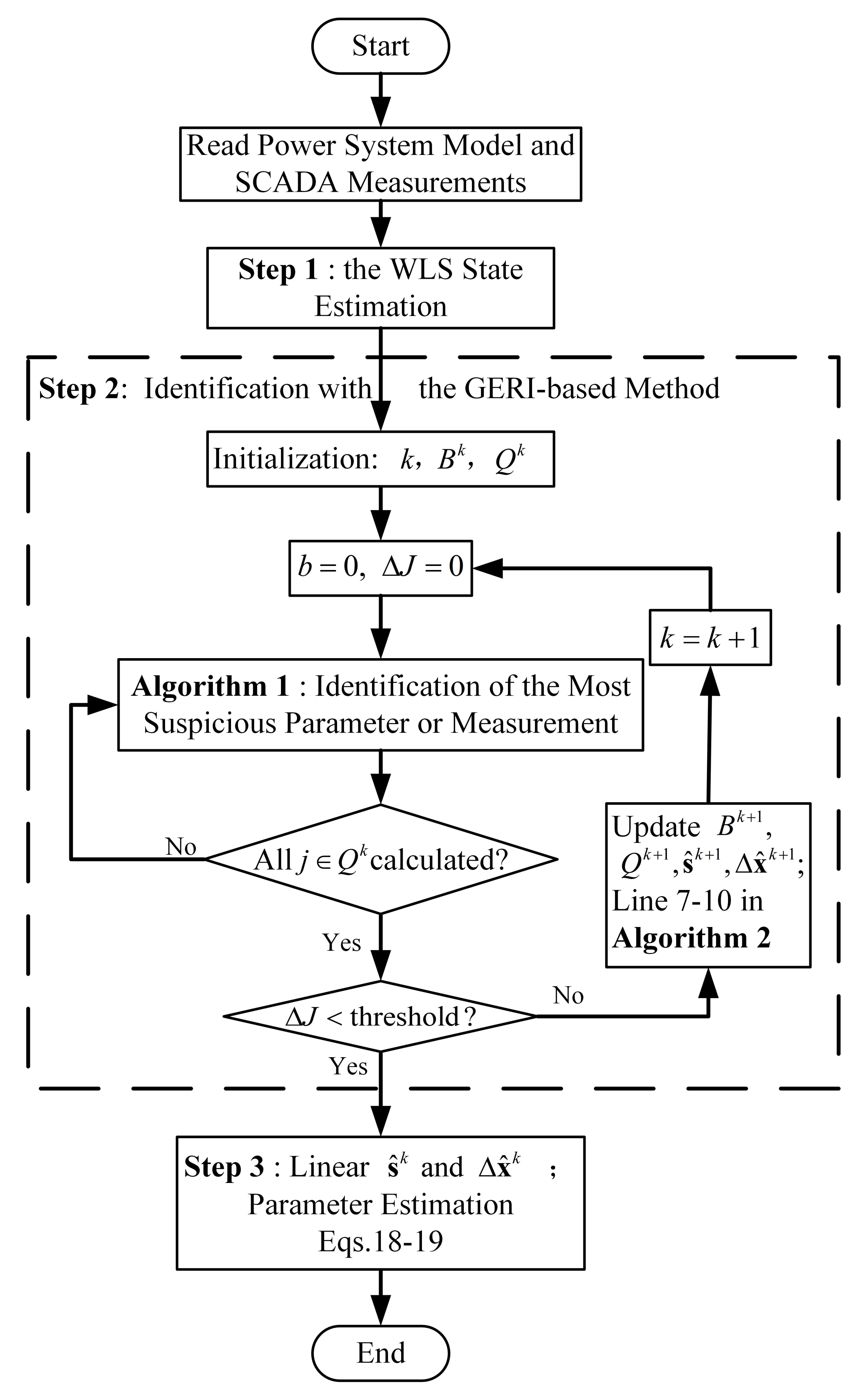
2.4. Flowchart of the GERI-Based Method

The whole algorithm contains three key steps: Step 1—the WLS state estimation; Step 2—identification with the GERI-based method; Step 3—parameter estimation via augmented SE. The measurements are acquired from the supervisory control and data acquisition system and mainly include voltage amplitudes, branch current amplitudes, active power flow, and reactive power flow.

Figure 1 shows the flowchart of the GERI-based method.

Step 1—The WLS SE combined with the orthogonal transformation method is adopted to improve the numerical stability and computation efficiency [32]. With fast Givens rotations technique [33], ${{\mathbf{H}}_{\mathbf{x}}}^{\mathit{T}}\mathbf{W}{\mathbf{H}}_{\mathbf{x}}$, the most important factor in WLS SE and our identification can be computed faster. ${{\mathbf{H}}_{\mathbf{x}}}^{\mathit{T}}\mathbf{W}{\mathbf{H}}_{\mathbf{x}}$ is output for the simplified calculation of the variables ($\widehat{s}$ and $\Delta \widehat{\mathbf{x}}$). $\mathbf{W}$, ${\mathbf{H}}_{\mathbf{x}}$, ${\mathbf{x}}^0$, ${\mathbf{r}}^0$, $\Delta \mathbf{x}$, and $\mathit{J}({\mathbf{x}}^0,0)$ are the inputs for Algorithm 2. In comparison with the NLM method, the GERI-based method only requires one run of the WLS SE. Thus, Step 1 is only run once.

Step 2—With the WLS SE results, the gross errors and the GERI indexes are calculated with the parameters and measurements from multiple measurement scans in Algorithm 1. Then, Algorithm 1 gains the most suspicious parameters and the maximum GERI by comparing all the indexes in Algorithm 1. Algorithm 2 will find all the maximum GERI indexes less than the threshold from output of Algorithm 1 in Algorithm 2. With the GERI-based method, it will output the erroneous parameters and measurements identified for parameter estimation in the next step.

Step 3—Before parameter estimation, linear correction for $\mathbf{x}$ and $\mathbf{s}$ is performed by $\mathbf{x}={\mathbf{x}}^0+\Delta {\widehat{\mathbf{x}}}^{\mathit{k}}$ and $\mathbf{s}={\widehat{\mathbf{s}}}^{\mathit{k}}$. With the corrected $\mathbf{x}$ and $\mathbf{s}$, erroneous parameters and measurements in $B^{\mathit{k}}$ are estimated via augmented SE.

The proposed method is an extension of the WLS method, which makes it closely related to the WLS state estimator in Step 1. When we try to identify multiple erroneous general parameters, it is practical for the proposed method to be directly integrated into the WLS state estimator as an additional module. Furthermore, identification in Step 2 reuses the WLS SE results, which helps to increase the computation speed.

2.5. Relation to the Normalized Lagrange Multiplier Method

The NLM method can identify parameter errors accurately and efficiently. When we identify only one erroneous parameter, the GERI-based method is equivalent to the NLM method. The maximum GERI is equal to the square of the NLM index, $\Delta \mathit{J}={\lambda }_{\mathit{j}}^{NT}{\lambda }_{\mathit{j}}^N$.

According to Reference [18], a normalized Lagrange multiplier $\lambda$ of larger than 3 is an indication of an erroneous parameter. Hence, the maximum GERI of larger than 9 is the corresponding threshold for parameter identification.

Due to the length of the derivation, the proof process is placed in Appendix A. It selects the model of the NLM method cited in Reference [17].

3. Implementation of the Method in Practice

3.1. Simplified Calculation of Variables

As indicated by (14), $\mathbf{A}=\mathbf{I}-{\mathbf{H}}_{\mathbf{x}}{\left({{\mathbf{H}}_{\mathbf{x}}}^{\mathit{T}}\mathbf{W}{\mathbf{H}}_{\mathbf{x}}\right)}^{-1}{{\mathbf{H}}_{\mathbf{x}}}^{\mathit{T}}\mathbf{W}$. As $\mathbf{A}$ is a dense matrix, the calculation of ${\mathbf{A}}^{-1}$ will consume a large amount of time and memory. The method reduces the computation and storage burden of $\mathbf{A}$ by deriving and computing subsets of $\widehat{\mathbf{s}}$ and $\Delta \widehat{\mathbf{x}}$.

According to WLS SE in Step 1, ${{\mathbf{H}}_{\mathbf{x}}}^{\mathit{T}}\mathbf{W}{\mathbf{H}}_{\mathbf{x}}$, which is the key part of $\mathbf{A}$, can be simplified using the orthogonal transformation method [32] and the fast Givens rotations technique [33] as follows:

$${{\mathbf{H}}_{\mathbf{x}}}^{\mathit{T}}\mathbf{W}{\mathbf{H}}_{\mathbf{x}}={{\mathbf{H}}_{\mathbf{w}}}^{\mathit{T}}{\mathbf{H}}_{\mathbf{w}}={\left(\mathbf{Q}{\mathbf{H}}_{\mathbf{w}}\right)}^T\left(\mathbf{Q}{\mathbf{H}}_{\mathbf{w}}\right)={\mathbf{R}}^T\mathbf{R},$$

(23)

where ${\mathbf{H}}_{\mathbf{w}}={\mathbf{W}}^{1/2}{\mathbf{H}}_{\mathbf{x}}$; $\mathbf{Q}$ is the orthogonal transformation matrix; $\mathbf{R}$ is the sparse upper triangular matrix, $\mathbf{Q}{\mathbf{H}}_{\mathbf{w}}$.

Substituting (23) into $\mathbf{A}$:

$$\mathbf{A}=\mathbf{I}-{\mathbf{H}}_{\mathbf{x}}{\mathbf{R}}^{-1}{\mathbf{R}}^{-T}{{\mathbf{H}}_{\mathbf{x}}}^{\mathit{T}}\mathbf{W}.$$

(24)

By converting the calculation of the dense matrix ($\mathbf{A}$) into sparse matrices (${\mathbf{H}}_{\mathbf{x}}$, $\mathbf{R}$ and $\mathbf{W}$), we can improve the computation speed.

3.1.1. Simplified Calculation of $\widehat{s}$

As shown in (12), $\widehat{\mathbf{s}}={\left({{\mathbf{H}}_{\mathbf{s}}}^{\mathit{T}}\mathbf{W}\mathbf{A}{\mathbf{H}}_{\mathbf{s}}\right)}^{-1}{{\mathbf{H}}_{\mathbf{s}}}^{\mathit{T}}\mathbf{W}{\mathbf{Ar}}^0$.

To simplify the calculation of $\widehat{\mathbf{s}}$, we calculate its key parts: $\mathbf{A}{\mathbf{r}}^0$ and ${{\mathbf{H}}_{\mathbf{x}}}^{\mathit{T}}\mathbf{W}\mathbf{A}{\mathbf{H}}_{\mathbf{s}}$.

$$\begin{array}{cc}\hfill {\mathbf{Ar}}^0& ={\mathbf{r}}^0-{\underline{{\mathbf{H}}_{\mathbf{x}}{\underline{{\mathbf{R}}^{-1}{\underline{{\mathbf{R}}^{-T}{\underline{{{\mathbf{H}}_{\mathbf{x}}}^{\mathit{T}}{\underline{\mathbf{W}{\mathbf{r}}^0}}_1}}_2}}_3}}_4}}_5.\hfill \end{array}$$

(25)

The second term of (25) solves sparse matrix-vector iterative multiplication in the order indicated by the underlines.

For another key part, ${{\mathbf{H}}_{\mathbf{s}}}^{\mathit{T}}\mathbf{W}\mathbf{A}{\mathbf{H}}_{\mathbf{s}}$:

$$\begin{array}{c}\hfill {{\mathbf{H}}_{\mathbf{s}}}^{\mathit{T}}\mathbf{W}\mathbf{A}{\mathbf{H}}_{\mathbf{s}}={{\mathbf{H}}_{\mathbf{s}}}^{\mathit{T}}\mathbf{W}{\mathbf{H}}_{\mathbf{s}}-{{\mathbf{H}}_{\mathbf{s}}}^{\mathit{T}}\mathbf{W}{\mathbf{H}}_{\mathbf{x}}{\mathbf{R}}^{-1}{\mathbf{R}}^{-T}{{\mathbf{H}}_{\mathbf{x}}}^{\mathit{T}}\mathbf{W}{\mathbf{H}}_{\mathbf{s}}.\end{array}$$

(26)

Denote: $\mathbf{M}={\underline{{\mathbf{R}}^{-T}{\underline{{{\mathbf{H}}_{\mathbf{x}}}^{\mathit{T}}{\underline{\mathbf{W}{\mathbf{H}}_{\mathbf{s}}}}_1}}_2}}_3$, (26) can be simplified as:

$${{\mathbf{H}}_{\mathbf{s}}}^{\mathit{T}}\mathbf{W}\mathbf{A}{\mathbf{H}}_{\mathbf{s}}={{\mathbf{H}}_{\mathbf{s}}}^{\mathit{T}}\mathbf{W}{\mathbf{H}}_{\mathbf{s}}-{\mathbf{M}}^T\mathbf{M},$$

(27)

where $\mathbf{M}$ is the sparse matrix and can be simply calculated in the order indicated by the underlines.

Substitute ${\mathbf{Ar}}^0$ (25) and ${{\mathbf{H}}_{\mathbf{s}}}^{\mathit{T}}\mathbf{W}\mathbf{A}{\mathbf{H}}_{\mathbf{s}}$ (27) into $\widehat{\mathbf{s}}$ (12):

$$\begin{array}{cc}\hfill \widehat{\mathbf{s}}=& {({{\mathbf{H}}_{\mathbf{s}}}^{\mathit{T}}\mathbf{W}{\mathbf{H}}_{\mathbf{s}}-{\mathbf{M}}^T\mathbf{M})}^{-1}{{\mathbf{H}}_{\mathbf{s}}}^{\mathit{T}}\mathbf{W}\times ({\mathbf{r}}^0-{\mathbf{H}}_{\mathbf{x}}{\mathbf{R}}^{-1}{\mathbf{R}}^{-T}{{\mathbf{H}}_{\mathbf{x}}}^{\mathit{T}}{\mathbf{Wr}}^0).\hfill \end{array}$$

(28)

3.1.2. Simplified Calculation of $\Delta \widehat{\mathbf{x}}$

As shown in (13), $\Delta \widehat{\mathbf{x}}$ contains two key parts: ${{\mathbf{H}}_{\mathbf{x}}}^{\mathit{T}}\mathbf{W}{\mathbf{H}}_{\mathbf{x}}$ (23) and $\widehat{\mathbf{s}}$ (28). Hence, $\Delta \widehat{\mathbf{x}}$ is given by:

$$\begin{array}{c}\hfill \Delta \widehat{\mathbf{x}}={\underline{{\mathbf{R}}^{-1}{\underline{{\mathbf{R}}^{-T}{\underline{{{\mathbf{H}}_{\mathbf{x}}}^{\mathit{T}}{\underline{\mathbf{W}{\underline{({\mathbf{r}}^0-{\mathbf{H}}_{\mathbf{s}}\widehat{\mathbf{s}})}}_1}}_2}}_3}}_4}}_5.\end{array}$$

(29)

$\Delta \widehat{\mathbf{x}}$ can be calculated directly and easily in the order indicated by the underlines in (29).

With the simplified calculation of the variables above, we can calculate $\widehat{\mathbf{s}}$ and $\Delta \widehat{\mathbf{x}}$ directly and avoid calculating the dense matrix $\mathbf{A}$. The main computation part of $\widehat{\mathbf{s}}$ and $\Delta \widehat{\mathbf{x}}$ is $\mathbf{R}$, which is calculated in WLS SE. As $\mathbf{R}$ is a sparse upper triangular matrix, the calculations of variables ($\widehat{\mathbf{s}}$ and $\Delta \widehat{\mathbf{x}}$) only needs to utilize sparse forward-backward iterations, which reduces the computation time and memory requirements.

3.2. Multiple Measurement Scans

Consider a set of N measurement scans. Each measurement residual vector for scan i is expressed as follows:

$$\begin{array}{c}\hfill {\mathbf{r}}^i={\mathbf{z}}^i-{\mathbf{h}}^i({\mathbf{x}}^i,{\mathbf{p}}_{\mathbf{e}})-{{\mathbf{v}}_{\mathbf{e}}}^{\mathit{i}}\forall i\in \{1,2,\cdots ,N\},\end{array}$$

(30)

where i, N, ${\mathbf{r}}^i$, ${\mathbf{z}}^i$, ${\mathbf{h}}^i({\mathbf{x}}^i,{\mathbf{p}}_{\mathbf{e}})$, and ${{\mathbf{v}}_{\mathbf{e}}}^{\mathit{i}}$ are defined in

Table 1. Definition for variables.

Variable	Definition
i	the measurement scan index
N	the number of measurement scans
${\mathbf{z}}^i$	the measurement vector for scan i
${\mathbf{h}}^i({\mathbf{x}}^i,{\mathbf{p}}_{\mathbf{e}})$	the nonlinear function relating the measurements of
	scan i to the system states for scan i and the network
	parameter errors
${\mathbf{p}}_{\mathbf{e}}$	the parameter error vector
${\mathbf{x}}^i$	the system state vector for scan i, including
	voltage magnitudes and phase angles
${\mathbf{v}}_{\mathbf{e}}^i$	the suspected measurement error vector for scan i
${\mathbf{r}}^i$	the measurement residual vector for scan i

.

Let us define the following vectors associated with the N scans:

$$\mathbf{r}=\left[\begin{array}{c}{\mathbf{r}}^1\\ {\mathbf{r}}^2\\ ⋮\\ {\mathbf{r}}^N\end{array}\right],\mathbf{z}=\left[\begin{array}{c}{\mathbf{z}}^1\\ {\mathbf{z}}^2\\ ⋮\\ {\mathbf{z}}^N\end{array}\right],\mathbf{x}=\left[\begin{array}{c}{\mathbf{x}}^1\\ {\mathbf{x}}^2\\ ⋮\\ {\mathbf{x}}^N\end{array}\right],{\mathbf{v}}_{\mathbf{e}}=\left[\begin{array}{c}{{\mathbf{v}}_{\mathbf{e}}}^1\\ {{\mathbf{v}}_{\mathbf{e}}}^2\\ ⋮\\ {{\mathbf{v}}_{\mathbf{e}}}^{\mathit{N}}\end{array}\right],$$

$$\mathbf{h}(\mathbf{x},{\mathbf{p}}_{\mathbf{e}})={\left[\begin{array}{cccc}\mathbf{h}{(\mathbf{x},{\mathbf{p}}_{\mathbf{e}})}^1& \mathbf{h}{(\mathbf{x},{\mathbf{p}}_{\mathbf{e}})}^2& \cdots & \mathbf{h}{(\mathbf{x},{\mathbf{p}}_{\mathbf{e}})}^N\end{array}\right]}^T.$$

The method of using multiple measurement scans to identify general parameter errors via the GERI-based method is similar to that of using a single measurement scan. Multiple measurement scans increase the redundancy of measurements and improve the parameter identification accuracy. However, the influences of multiple measurement scans on erroneous parameters and measurements are different.

If a single erroneous parameter exists, it is relatively constant and will affect the gross error of each scan. Hence, parameter errors can be considered as deterministic variables and their sum influence can be calculated when multiple measurement scans are considered simultaneously. This, therefore, makes erroneous parameters far easier to identify.

If a single erroneous measurement exists, the GERI index is independent of the number of measurement scans made. Using multiple measurement scans increases the redundancy of measurements for identification.

In addition, identification with multiple measurement scans has the same number of $\mathbf{x}$ as the augmented state variables compared with a single scan. However, it improves the identification accuracy and numerical stability by increasing the redundancy in SE.

4. Simulation Results

The GERI-based method identifies erroneous measurements simultaneously based on the identification of erroneous parameters. To illustrate the performance and limitation of this method, its procedure is implemented and tested in an IEEE 14-bus test system and a real power system model of the Eastern Grid in China. Several matpower cases are simulated to further analyze the computation speed of this method in large-scale power systems. In the following simulations, the error covariance is assumed to be 0.01 p.u. for all measurements and the parameter values are in p.u. Except for assumed errors in each case, no deviations are introduced in other parameters or measurements. To improve the implementation of the proposed method, cases consider power flow measurements of 6 scans at load levels of 0.7, 0.8, 0.9, 1.0, 1.1, and 1.2.

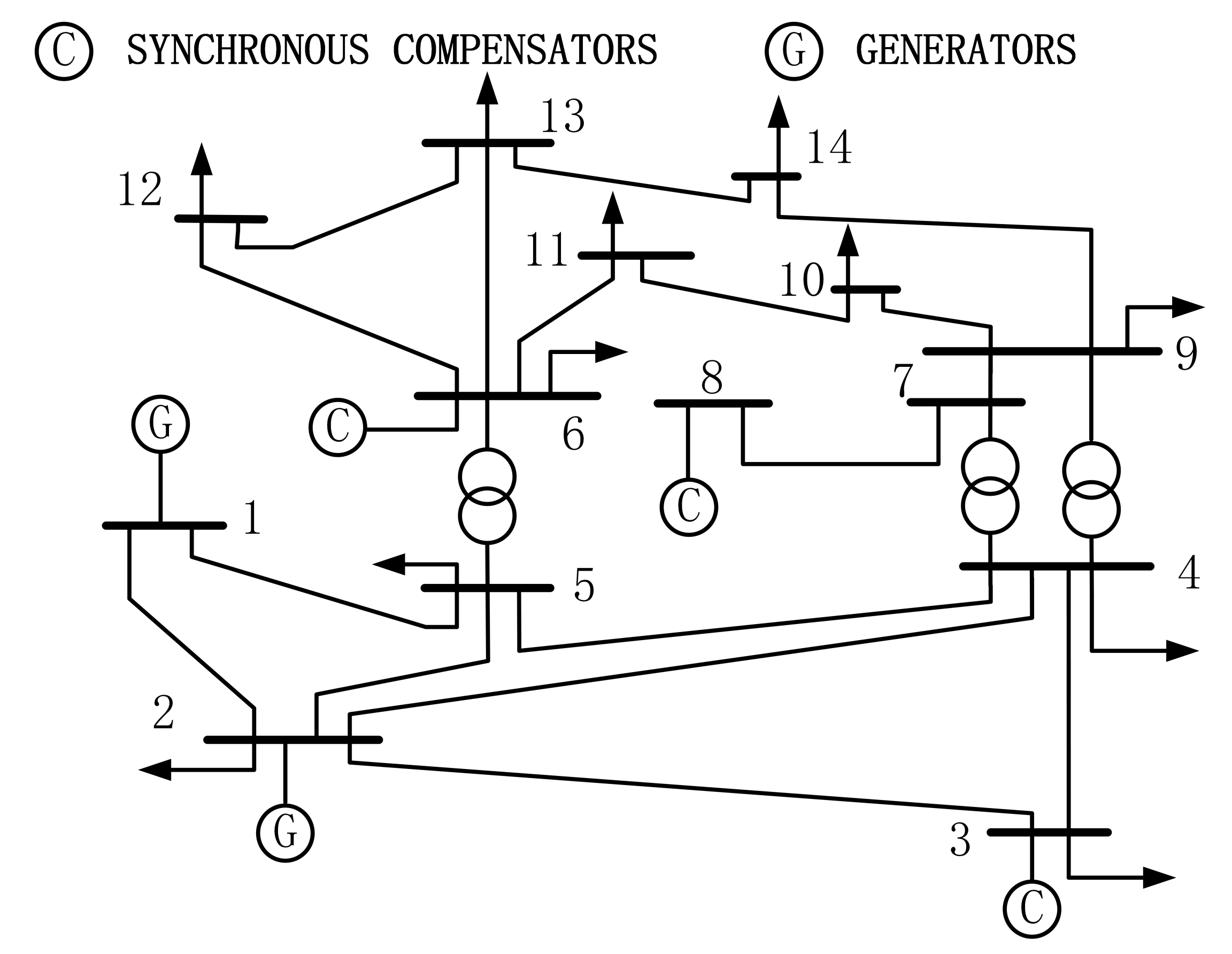
4.1. Simulations of the IEEE 14-Bus Test System

The IEEE 14-bus test system has 14 buses, 20 branches, and 123 measurements, as depicted in Figure 2. All measurements were taken from the WLS SE; are considered to increase redundancy; and contain 1 phase ($\theta$), 14 node voltage values ($V_{\mathit{j}}$), 14 node power flow values ($P_{\mathit{j}}$), 14 node reactive power flow values (${\mathit{Q}}_{\mathit{j}}$), 40 power flow values ($P_{i\mathit{j}},P_{\mathit{j}i}$), and 40 reactive power flow values (${\mathit{Q}}_{i\mathit{j}},{\mathit{Q}}_{\mathit{j}i}$).

Different types of errors are adopted to test the identification effect of the method in three cases.

4.1.1. Case 1: Identification of a Single General Parameter Error

This case identifies all single general parameter errors by adding an assumed general parameter relative error to the true parameter or measurement. The assumed general parameter relative error refers to the ratio of general parameter error (s) to the true number of parameters or measurements.

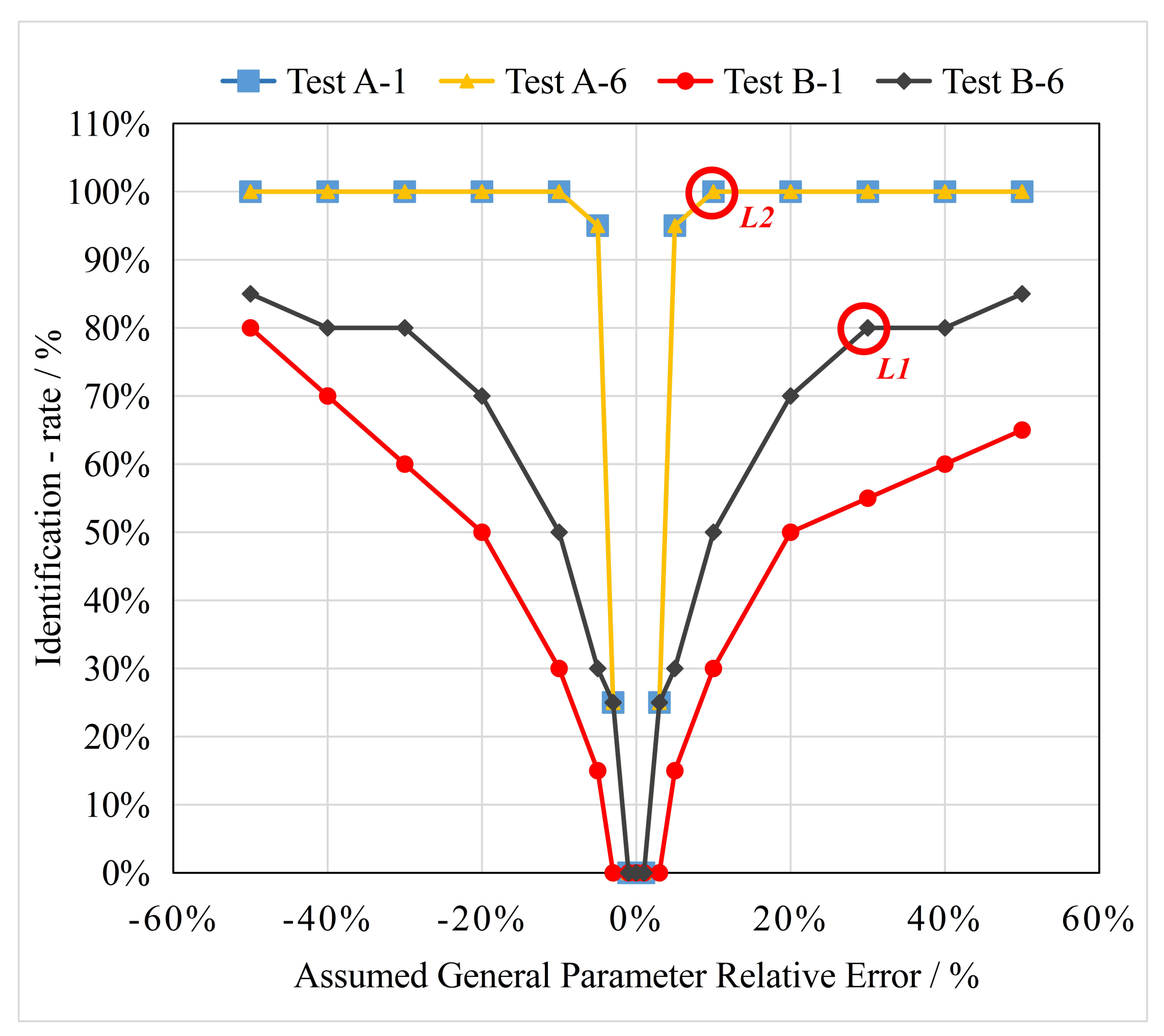
Figure 3 presents the relation between the identification-rate and the assumed general parameter relative error. The identification rate refers to the ratio of the number of identified erroneous parameters and measurements to the total number of parameters and measurements. A single scan is used in Test A-1 and Test B-1, while six scans are used in Test A-6 and Test B-6. Tests A and B in Figure 3 are carried out as follows:

Test A: Different relative errors are introduced in single measurements ($P_{i\mathit{j}}$); all parameters are error-free.

Test B: Different relative errors are introduced in single parameters ($X_{i\mathit{j}}$); all measurements are error-free.

According to Test A, the proposed method identifies the single measurement error when the relative error is larger than or equal to $\pm 5\%$, and no single measurement error is identified when the relative error is less than or equal to $\pm 1\%$. Although multiple measurement scans increase the redundancy of measurements, they have no effect on the identification-rate for a single measurement error in Figure 3. According to Test B, the identification-rate for a single parameter error increases with the relative error. With six scans, the method identifies more single erroneous parameters than with a single scan. Text B-6 is also more beneficial to small parameter errors between +3%–+5% and $-3\%$–$-5\%$ than Text B-1. The adoption of multiple measurement scans increases the identification-rate for a single parameter error, as stated in Section 3.2.

For +30% error added to each parameter ($L1$ in Figure 3) and +5% error added to each measurement ($L2$ in Figure 3),

Table 2. Single error identification results for the NLM method and the GERI-based method with a single scan.

Assumed	the NLM Method		the GERI-Based Method
General	Index	Identified	Index	Identified	${\mathit{\lambda }}^2$/$\mathbf{\Delta }\mathit{J}$
Parameter	/$\mathit{\lambda }$	($\mathit{\lambda }\ge 3$)	/$\mathbf{\Delta }\mathit{J}$	($\mathbf{\Delta }\mathit{J}\ge 9$)
$X_{1-5}$	23.891	$X_{1-5}$	570.773	$X_{1-5}$	1.000012
$X_{13-14}$	1.455	$NO$	2.117	$NO$	1.000012
$P_{2-5}$	4.785	$P_{2-5}$	22.895	$P2-5$	1.000054
${\mathit{Q}}_{2-5}$	4.773	${\mathit{Q}}_{2-5}$	22.786	$\mathit{Q}2-5$	0.999804

shows the partial identification results obtained with the NLM method and the GERI-based method with a single scan. The 2nd column presents the normalized residual index ($\lambda$) and the 3rd column presents the identified erroneous parameters and measurements when $\lambda \ge 3$. The 4th column presents the GERI index ($\Delta \mathit{J}$) and the 5th column presents the identified erroneous parameters and measurements when $\Delta \mathit{J}\ge 9$. The 6th column presents the ratio of ${\lambda }^2$ to $\Delta \mathit{J}$. It is obvious that the deduction of the relation between the NLM method and the GERI-based method in Appendix A is correct; thus, ${\lambda }^2=\Delta \mathit{J}$. For the erroneous reactance of branch 13–14, values of $\lambda$ and $\Delta \mathit{J}$ are too small to identify $X_{13-14}$. However, general parameter errors on branch 1–5 and 2–5 can be identified correctly with both methods.

4.1.2. Case 2: Identification of a Single Parameter Error with an Adjacent Measurement Error

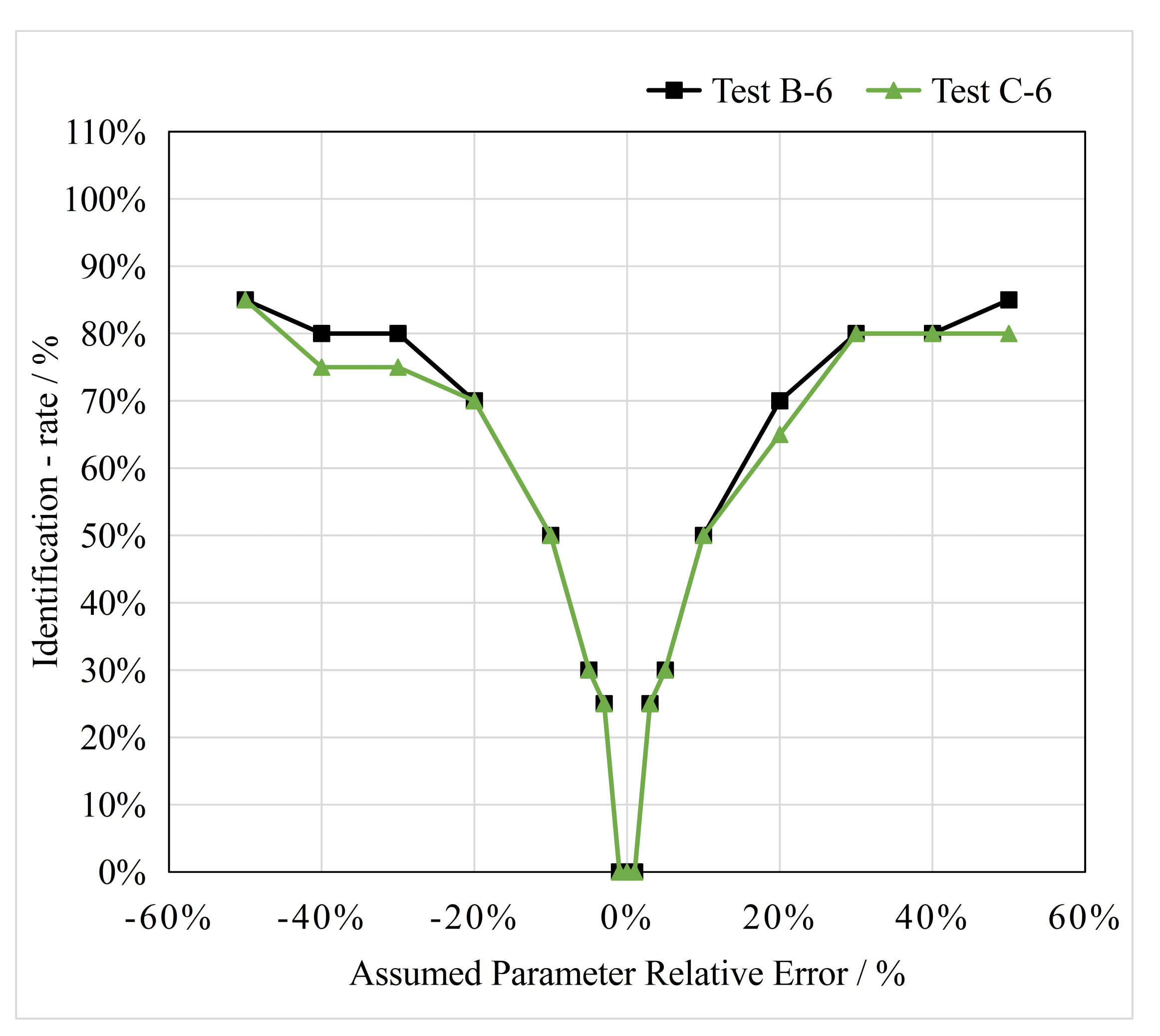
This case identifies all the single erroneous parameters ($X_{i\mathit{j}}$) with an adjacent erroneous measurement ($P_{i\mathit{j}}$) by adding an assumed parameter relative error to the true parameter. The assumed parameter relative error refers to the ratio of parameter error (s) to true parameter value. If the erroneous $X_{i\mathit{j}}$ and $P_{i\mathit{j}}$ are identified simultaneously, the identification case is correct. Identification-rate refers to the ratio of correctly identified cases to the total number of cases.

Figure 4 presents the identification-rate of Test B-6 and Test C-6. Test B-6 is equal to Test B-6 in Figure 3. Test C-6 is as follows.

Test C-6: Different assumed parameter relative errors are added to the parameters when their adjacent measurement error is $5\%$. Six scans are used for identification.

When measurement error and parameter error exist at the same time, it is most difficult to identify the correlation between them, as the two errors have a similar effect on the SE. According to Test C-6, negative effects of $X_{i\mathit{j}}$ and $P_{i\mathit{j}}$ can be distinguished with the GERI indexes. Compared with Test B-6, Test C-6 can increase the identification-rate for Case 2 by improving the identification-rate for a single erroneous parameter.

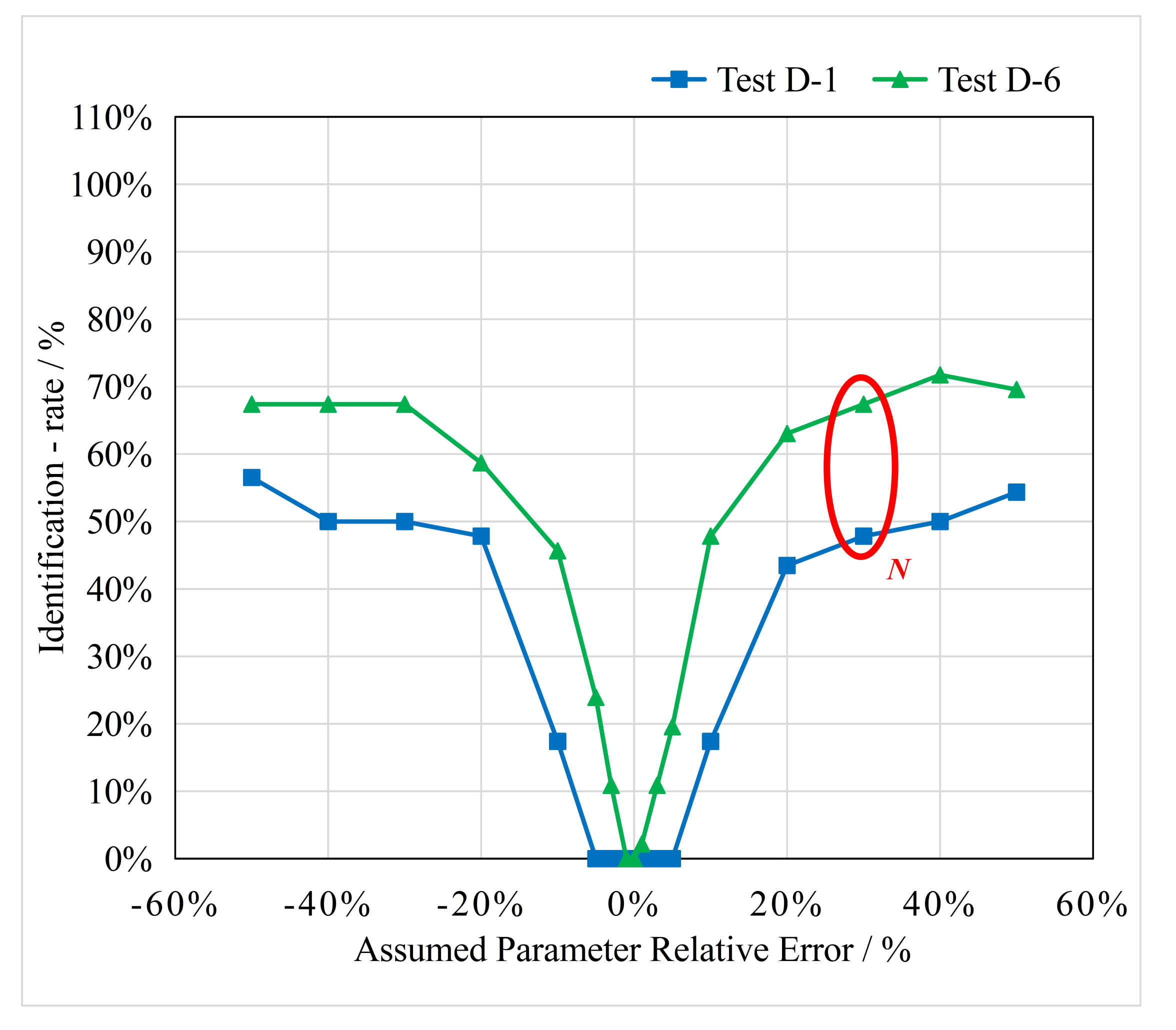
4.1.3. Case 3: Identification of Two Adjacent Parameter Errors

This case presents the identification-rate for two adjacent parameter errors ($X_{i\mathit{j}}$ and $X_{i\mathit{k}}$) existing simultaneously with same assumed parameter errors. Test D adds different assumed parameter relative errors to two adjacent parameters ($X_{i\mathit{j}}$ and $X_{i\mathit{k}}$). For each $X_{i\mathit{j}}$ and $X_{i\mathit{k}}$, the errors are the same. The difference between Test D-1 and Test D-6 is as follows:

Test D-1: A single scan is used for identification.

Test D-6: Six scans are used for identification.

According to Figure 5, this method can identify more parameters with an increasing parameter relative error. The adoption of six scans generally improves the identification-rate for two adjacent parameter errors and the identification of minor parameter relative error between $-5\%$ and $+5\%$.

For N in Figure 5,

Table 3. Identification of two adjacent erroneous parameters with assumed $30\%$ errors.

	Identified Cycle	Identified Parameter	GERI Index	Exact Value/p.u.	Estimated Value/p.u.	Estimation Error/p.u.
With a	1	$X_{5-6}$	34.126	0.25202	0.278599	0.026579
single	$NO$	$X_{4-7}$	$<9$	0.20912	0.250944	0.041824
scan	$NO$	$X_{4-9}$	$<9$	0.55618	0.667416	0.111236
With	1	$X_{5-6}$	185.203	0.25202	0.25202	0
six	2	$X_{4-9}$	25.492	0.20912	0.20912	0
scans	3	$X_{4-7}$	68.652	0.55618	0.55618	0

displays the identification results of two erroneous line reactances ($X_{4-7}$ and $X_{4-9}$) with assumed $30\%$ errors. The 2nd column indicates the cycle of erroneous parameters identified. The 3rd column shows the identified erroneous parameter, and the 4th column shows its GERI index. The 5th column indicates exact values, and the 6th column indicates estimated values. The estimation errors in the 7th column are equal to the estimated values minus exact values. With a single scan, $X_{4-7}$ and $X_{4-9}$ are unidentified because their GERI indexes are less than 9, which is the threshold. $X_{5-6}$ is over-identified. Hence, there are estimation errors after linear correction and parameter estimation. With six scans, $X_{5-6}$ is still over-identified but $X_{4-7}$ and $X_{4-9}$ are correctly identified. The over-identification of $X_{5-6}$ does not affect their correct estimation. It is apparent that multiple measurement scans do help to identify two adjacent erroneous parameters and gain correct estimation values.

4.2. Simulations of the Eastern Grid in China

This case comprises tests on a model of a real power system, the Eastern Grid in China. The Eastern Grid has 6023 buses, 9557 branches, 2454 loads, 72,270 states, and 337,788 measurements, as shown in

Table 4. Scale of simulation for the Eastern Grid in China.

Type	Number
Buses	6023
Branches	9557
Generators	658
Loads	2454
Total states	72,270
Total measurements	337,788
Measurement Scans	6
Introduced erroneous parameters	10

. The initial power flow result is obtained from power flow calculation using offline data. To ensure the identification effect, the power flow results at six measurement scans are similarly used to identify multiple erroneous parameters. This runs on a laptop with an Intel (R) Core ($TM$) i7-4710 $M\mathit{Q}$ [email protected] G Hz and 8.00 GB of RAM.

To test the identification results and calculation efficiency of the proposed method in large-scale power systems, 10 randomly generated erroneous parameters were designed in this case with six measurement scans. The values of these erroneous parameters are their exact values plus $30\%$.

Table 5. Parameter identification results for the Eastern Grid in China.

Cycle	Error Type	Identified Parameter	Gross Error	GERI
1	parameter	$X_{621-622}$	523,705	281,764
2	parameter	$X_{1667-1670}$	241,941	212,557
3	parameter	$X_{3325-3328}$	29,384	7458
4	parameter	$X_{2874-2875}$	21,926	6110
5	parameter	$X_{4355-4357}$	15,816	4869
6	parameter	$X_{15-16}$	10,947	4672
7	parameter	$X_{1667-1678}$	6275	2359
8	parameter	$X_{2991-2993}$	3916	2166
9	parameter	$X_{5077-5080}$	1750	751
10	parameter	$X_{324-325}$	999	730
11	measurement	$P_{621-622}$	269	34
12	measurement	$P_{3325-3328}$	235	25
13	measurement	$P_{15-16}$	210	18
14	measurement	$P_{4355-4357}$	192	13
15	measurement	$P_{5077-5080}$	179	9

shows 1st the parameter identification results obtained from the Eastern Grid in China. The 1st column indicates the identified cycle of general parameter error. Error type is shown in the 2nd column. The 3rd column indicates the identified parameter. The 4th column gives the gross error of the identified erroneous parameter. The GERI index in the 5th column is equal to the gross error of the current cycle minus that of the next cycle, as is shown in (17). We note that all random erroneous parameters are identified simultaneously. Although $X_{1667-1670}$ relates to $X_{1667-1678}$, both are identified correctly without over-identification. However, five additional measurements are over-identified for linearization-induced errors in the nonlinear model.

To analyze the adverse effects of over-identification,

Table 6. Parameter estimation results for the Eastern Grid in China.

Cycle of Parameter Identified	Assumed Erroneous Parameter Value/p.u.	Estimated Parameter Value /p.u.	Exact Parameter Value /p.u.	Estimation Error /p.u.
1	0.007161	0.01023	0.01023	0.000000
2	0.007364	0.01052	0.01052	0.000000
3	0.007490	0.01070	0.01070	0.000000
4	0.007490	0.01070	0.01070	0.000000
5	0.008218	0.01174	0.01174	0.000000
6	0.008939	0.01277	0.01277	0.000000
7	0.011158	0.01594	0.01594	0.000000
8	0.012712	0.01816	0.01816	0.000000
9	0.017780	0.02540	0.02540	0.000000
10	0.025354	0.03622	0.03622	0.000000

shows the parameter estimation results. The 1st column gives the cycle of parameter identified. The 2nd column shows the value of the assumed erroneous parameter. The 3rd column presents the estimated parameter value obtained via augmented SE. The 4th column presents the exact parameter value. The estimation error is given in the 5th column. By comparing the estimated parameter values and exact parameter values, it can be observed that the estimation errors of 10 erroneous parameters are all equal to 0. Thus, over-identification in Table 5 does not affect the estimation results of parameters when multiple erroneous parameters are accurately identified. The GERI-based method performs well in identifying multiple erroneous parameters simultaneously.

Table 7. Computation time of simulation for the Eastern Grid in China.

Procedure	Time (s)
Step 1: State Estimation	4.48
Step 2: Parameter Identification	45.87
Step 3: Parameter Estimation	2.07
Total	52.42

provides the detailed computation time of each step of the simulation for the Eastern Grid test system. For large-scale power systems, parameter identification accounts for the greatest computation time. It takes about 45.87 s to detect 10 erroneous parameters from 9557 line reactances simultaneously with a simplified calculation of variables in Section 3.1. The GERI-based method only requires one run of WLS SE, which takes about 4.48 s. Compared with the method that requires SE for each identification, the proposed method reduces 14 SEs and saves about 62.7 s. Hence, the proposed method can be practically applied in a bulk power system, as it requires less memory and less computation time.

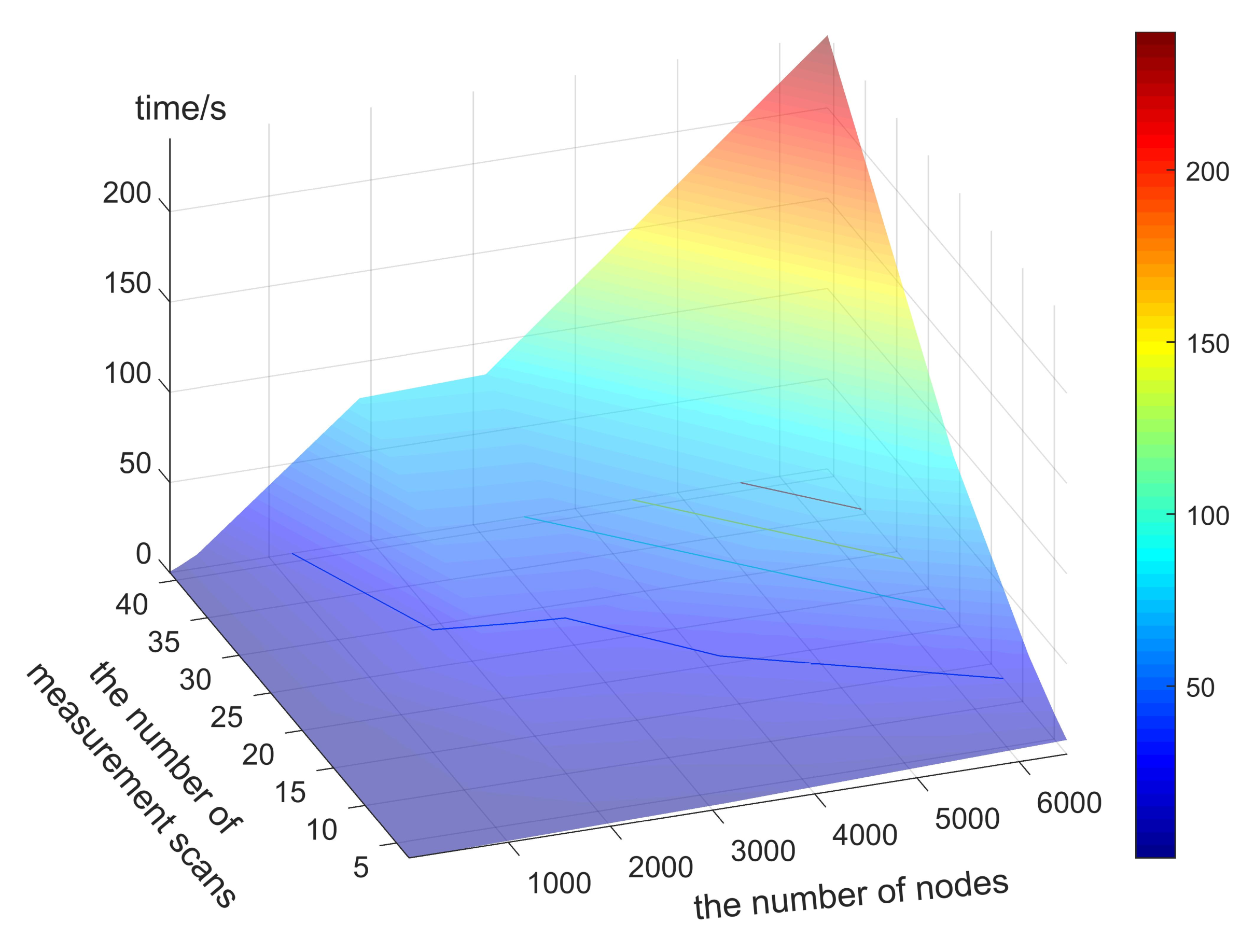
4.3. Simulations of Several Matpower Cases

This simulation applies six matpower files: case 14 (power flow data for the IEEE 14 bus test case), case 30 (power flow data for 30 bus, 6 generator case), case 118 (power flow data for the IEEE 118 bus test case), case 300 (power flow data for the IEEE 300 bus test case), case 1888rte (AC power flow data for the French system), case 3120sp (power flow data for the Polish system—summer 2008 morning peak), and case 6468rte (AC power flow data for the French system).

To compare the computation time when a different number of nodes and a different number of measurement scans are used, we introduced a randomly generated erroneous parameter with an assumed $30\%$ error in each case.

With the single erroneous parameter identified in all cases, Figure 6 shows that the computation time increases when the number of nodes or the number of measurement scans increase. For a system with below 1000 nodes, erroneous parameters can be identified within 50 s by using 41 measurement scans. For a system with 6000 nodes, it takes within 50 s using 10 measurement scans. With multiple measurement scans, we need to select the appropriate number of measurement scans to balance the identification effect and computation speed.

5. Conclusions

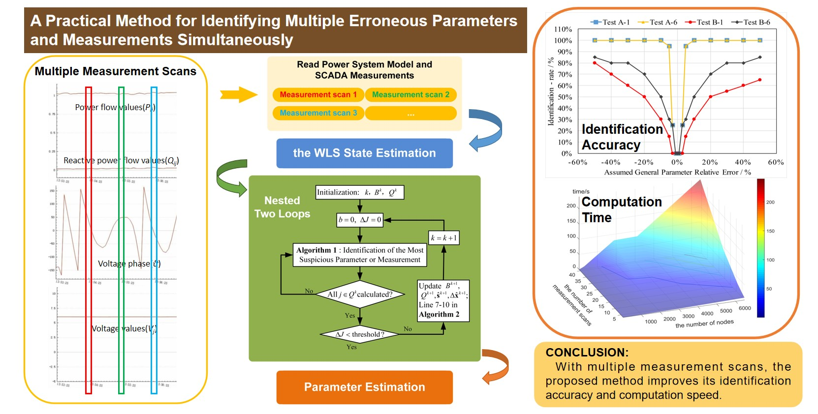
A practical GERI-based method is proposed to identify multiple erroneous parameters and measurements simultaneously for the existing static-state estimator. As an additional functional module, it can be applied quickly and effectively when needed. If administrators have doubts about the accuracy of parameters, the proposed method can be carried out to identify erroneous parameters and eliminate their adverse effects. The simulation of the IEEE 14-bus test system shows the identification effect of three cases. The identification of a single general parameter error, a single parameter error with an adjacent measurement error, and two adjacent parameter errors verify the accuracy of the GERI-based method. Multiple measurement scans increase the redundancy of measurements and help to identify multiple erroneous parameters. The simulation of the Eastern Grid in China indicates that the GERI-based method can identify multiple erroneous parameters accurately in large-scale power systems and performs quite well in terms of computation cost. Simulations of several matpower cases can improve the computation speed by selecting a suitable number of measurement scans.

At present, the proposed identification method has been commissioned for use in six provincial power grids in China. By introducing phasor data from phasor measurement units and testing to find the appropriate number of measurement scans, we will further improve the identification effect and computation speed of this method.