Abstract
This paper presents issues related to the adaptive control of the drive system with an elastic clutch connecting the main motor and the load machine. Firstly, the problems and the main algorithms often implemented for the mentioned object are analyzed. Then, the control concept based on the RNN (recurrent neural network) for the drive system with the flexible coupling is thoroughly described. For this purpose, an adaptive model inspired by the Elman model is selected, which is related to internal feedback in the neural network. The indicated feature improves the processing of dynamic signals. During the design process, for the selection of constant coefficients of the controller, the PSO (particle swarm optimizer) is applied. Moreover, in order to obtain better dynamic properties and improve work in real conditions, one model based on the ADALINE (adaptive linear neuron) is introduced into the structure. Details of the algorithm used for the weights’ adaptation are presented (including stability analysis) to perform the shaft torque signal filtering. The effectiveness of the proposed approach is examined through simulation and experimental studies.
1. Introduction
The continuous development of industrial processes’ automation creates demand for precision, speed and consequently, higher productivity [1,2]. Industrial automation is based mainly on different types of electrical servo systems. In electrical drives, usually, the cascade control concept is implemented. The control structure is divided into two or three main loops. The inner loop is responsible for suitable fast electromagnetic torque control. It can have different structure, depending on the driving motor. For example, it can be realized by a current controller for the DC motor or a FOC structure for the induction motor. The outer loop(s) realize the speed (position) control task [3,4]. Depending on the type of the mechanical structure, a simple PI controller (one-mass system) or more advanced concepts (multi-mass system) can be implemented. The type of the specific control algorithm depends on the design requirements and operation condition of the drive. It can be complicated in the case of system parameter uncertainty, noise levels, types of sensors and a lack of the information of selected system states (thus a special estimator is needed to estimate the unmeasurable signals).
Electrical drive systems can be divided into many groups, taking into account different factors. One possible portion criterion is the type of mechanical connection between the driving motor and the load machine. In the case of a stiff connection, the model of the mechanical part takes the simplest form. It consists of one rotating mass, which encompasses the electrical motor, and a load machine. Obviously, it means that the speed of the driving motor is equal to the speed of the load machine. This model is called a one-mass system in the literature. When the speed of the driving motor is different from the speed of the load machine, a more complicated model, called a two-mass system, should be used. In this case, the mechanical shaft is characterized by a finite stiffness coefficient. The characteristic problems which occur here are torsional vibrations, and they negatively influence the system performances. Firstly, they influence the reliability of the whole drive system, and additional limits of shaft torque amplitude are required in this drive. Secondly, the speed and the position accuracy of the motion control system are affected. In addition, the vibrations can negatively influence the working environment [5,6,7,8,9,10,11,12,13].
In order to successfully suppress torsional vibrations, different approaches have been developed over the years. In general, they can be divided into passive and active frameworks. The first comprises concepts based on the application of additional mechanical dampers, which increase the damping coefficient of the system. Although those approaches allow to successfully suppress vibrations, they also possess some disadvantages. Firstly, they increase the total cost of the system, and secondly, there must be a place to fix the mechanical damper to the system. The active frameworks are based on the implementation of special control algorithms. The classical controller for a standard electrical drive is based on the classical PI/PID concept. This approach is efficient only for a one-mass system with constant parameters and negligible nonlinearities. Since it is not effective enough for the two-mass system, some solutions have been proposed in the literature. The simplest approach for the structure with a PI controller is based on an alternative location of the system closed-loop poles. Since the double (classical) location is not effective, the poles can be placed on a circle or line with an identical real part or damping coefficient [9,10]. These locations can increase the damping ability of the control system, but only within a limited range of parameters. The authors also considered the application of a PID controller [9]. In this case, the designer has three control coefficients, so the independent location of four closed-loop poles is still not possible. More extensive research concerning the use of a PID controller for vibration damping of the two-mass system is presented in [10]. The author considers systems with different resonance ratios. Based on the research, the author concludes that there is a fundamental performance limitation in the case of a PI/PID controller. The systems with low and high resonance ratios are hard to control, as the response of the system is poorly damped or sluggish. The closed-loop bandwidth is limited by the value of anti-resonant frequency. The derivative feedback can be used to improve the damping ability of the system. The cut-off frequency of the low-pass filter in the derivative part has to be set according to the resonance frequency. The D part can partially improve the performance of the system; however, its use is limited due to the measurement noises.
In order to improve the performance of the control structure, other concepts have been proposed. The torsional vibrations can be successfully damped by inserting additional feedback from selected state variables to the system. In [11], nine additional feedbacks are analyzed. They are divided into three groups with identical damping abilities. Insertion of one additional feedback allows to successfully suppress vibrations, however the settling time of the load speed cannot be set freely. In order to locate the closed-loop system poles in a desired position, there is a need to use two additional feedbacks from selected variables [11]. A similar performance can be ensured using a state controller. The location of the system closed-loop poles influence the characteristics of the drive, so it is a significant point during the design procedure [12,13]. In [14,15], the forced dynamic control structure is proposed. It allows to locate the system closed-loop poles in a desired position and additionally eliminate (rather in theory) the influence of the load torque on the load speed. This damps the oscillations caused by a changeable load torque. In the literature, there is a significant number of papers describing the control structure with disturbance observers. This approach is based on the estimated disturbance (shaft torque) and feeds it back to the control structure. This allows to effectively damp oscillations [16,17,18].
For changeable parameters of the plant, more advanced control algorithms can be used, such as: adaptive control [3,19,20,21], sliding-mode control [22], predictive control [23,24] and others. The adaptive control can be generally divided into two main groups. The first one includes the so-called indirect methods. These control structures require additional identification blocks which calculate values of the changeable parameters of the plant. Then, based on these values, the new coefficients of the controller are calculated and updated. As an identification block, different methods can be applied. In [19], the Kalman filter is used to compute the changeable values of the time constant of the load machine. Based on this, the gains of the control structure with additional feedbacks are retuned. In the second framework, direct adaptive systems are included. Contrary to indirect methods, the identification block is not evident here. The controller parameters are retuned based on the output of the plant and the input of the system. In [3], two adaptive control structures with a fuzzy and sliding-fuzzy controller are analyzed. It is shown that the sliding version is more robust to parameter changes than the classical PI controller. The application of the Petri-nets can reduce the complexity of the fuzzy controller, as shown in [20]. In [21], the neural controller is proposed. The presented research proves it effectiveness, despite the simple structure of the controller. The sliding-mode control is known for its robustness against the changes of the plant parameters [22]. The next advanced control structure is based on model predictive control (MPC) [23,24]. This methodology has attracted much attention from the control community for the last few decades. On the basis of the model of the plant, the future behavior of the object is predicted. The optimization procedure allows to select the optimal control strategy in the time window. Applying the MPC allows to obtain optimal transients (according to the specified cost function) and at the same time, implement limitations of the control signal and the internal states of the plant. Additionally, examples of other, control methodologies can be found in the literature [25,26].
These control structures need information of system states. Since in industrial applications, only signals of electromagnetic torque and motor speed are available, there is a need to apply special estimation techniques [19,27,28,29], for example, the Luenberger observer, the Kalman filter and neural networks. However, these estimators are based (in the case of a two-mass system) on motor speed and current signals. Thus, the quality of measurement signals is still important.
Nowadays, with technology development, electrical drives have found many applications in various types of vehicles (cars, e-bikes, self-balancing scooters, traction systems, etc.) [30,31]. Typical issues evident in classical electrical drives (control methods, state variables’ estimation, hardware solutions) are significantly extended, including battery technology, mechanical connections, power consumption management, GPS location, slip control, etc. In [32], the sources of vibrations in a car and their impact on other components are analyzed. A generalized suppression strategy is proposed and tested during idle and cruising modes. The obtained results show good damping ability of the proposed method, with a small impact on the vehicle speed. The authors report that the strategy is also effective for different parameters of the car. Multi-sensor fusion based on a speed estimator is proposed in [33]. The combination of the wheel speed and GPS-BD module is considered. The authors claim that the proposed method has high accuracy and robustness. The hybrid control based on the acceleration slip regulation method is proposed in [34]. The four-wheel independent actuated electrical vehicles are considered here. The proposed method is based on the combination of slip-ratio and maximum-torque strategies. An adaptive torque search method is employed to improve performance at low speeds. For higher speeds, the sliding mode is implemented in order to regulate the slip ratio. An effective control technique is designed using the Lyapunov theory. Hardware-in-loop tests have shown that the proposed strategy possesses good performance under various driving conditions.
Artificial neural networks are algorithms that can be adapted to a specific task in an engineering application during the training process (adaptation of internal coefficients). The mentioned action introduces some flexibility in technical applications. On the basis of an appropriate dataset describing the relationships between the inputs and the outputs of the model, properties of a given neural network can be assigned [35]. This can lead to tunable circuits used for control, observation of state variables, signal prediction, measurement of noise removal or data analysis. This justifies the increasing number of applications of neural networks in various fields of science and industrial solutions. Obviously, among the applications of neural networks, the issues related to electrical drives are also often described in scientific publications [36,37,38]. The characteristic criterion according to which the analyzed implementations of neural networks can be divided is the calculation mode of the adaptation algorithm. The coefficients can be calculated on the basis of a previously collected dataset. Otherwise, the adaptation can be performed online. This means introducing corrections for the parameters of the neural network during operation of the entire system. The second approach seems more favorable. In this case, complex design problems are omitted (correct representations of the problem through training data are reduced, selection of neural network topology and training parameters (e.g., number of epochs), etc.). Due to the specificity of applications, the method of data processing in the neural network is also very important. Two fundamental groups of neural models differ from each other by the direction of data transmission within the structure. The first one takes into account only the signals from the previous network layer in the calculation of the output values of subsequent neurons. The second concept is to introduce feedback inside the network. Therefore, an additional component of the model is elements holding the previously processed values. This provides additional time-dependent information during calculations of output values. This is the reason why applications of recurrent neural networks are often used to analyze dynamic signals. There are different concepts about the inserted feedbacks. However, two types of recurrent neural networks dominate [39]. The first of them are called the Jordan neural networks, where a characteristic element is the introduction of a global coupling from the output layer to the input [40]. The second type of these models—the Elman network—usually contains one hidden layer in which the connection from the neuron outputs to the inputs of subsequent nodes is attached [41]. In this application, the Elman recurrent neural network is used as the basic structure applied in the speed controller of the electrical drive with compound mechanical part.
The control performance of the adaptive control structure depends on the measurement information. Different factors influence the quality of the sensor, for example resolution, linearity, response time, temperature range, sensitivity to additional noises and mechanical vibrations. Over time, the degradation of sensors can also be expected, from small to total deterioration. Those problems degrade the control method characteristics and can lead to instability of the whole control structure. In order to improve the quality of the measurement (or estimated) signals, a different approach can be used. In this paper, the ADALINE models [42,43,44] are applied. This adaptive structure allows to accomplish the above-mentioned tasks. The data space is linearly separated in the ADALINE model, and the calculations include weighted summation of the input values.
In this paper, the issues related to adaptive control for industrial drives with elasticity and changeable parameters are presented. At the beginning of the study, the inner loop (torque control loop) is assumed to be optimized and ensures fast torque responses. The adaptive controller is applied in an outer (speed) loop. The controller is based on RNN (recurrent neural network) and it is inspired by the Elman model. In order to select values of the control, the PSO (particle swarm optimizer) coefficient is applied. Additionally, the ADALINE (adaptive linear neuron) model is used in the system in order to reduce the noises evident in the control structure. Different research scenarios are considered. The systems with different (changeable) inertia of the load machine, elasticity of the flexible connection as well as imperfections in the torque control loop are considered. As a result, the on-line adaptive RNN controller has shown its good damping ability of torsional vibrations. The theoretical considerations are confirmed by a number of simulation as well as experimental studies.
The paper consists of seven main parts. The first section presents the scientific problem and motivation behind the work. Then, the mathematical model of the plant is briefly described. Next, the structure of the adaptive controller and the adaptation law are introduced. In the next section, the ADALINE model and its application as a signal filter based on this neuron are shown. Design issues related to the adaptive neural controller are also considered in the next section of the paper. For this purpose, the PSO algorithm is applied. The simulation and experimental studies show the work of the speed control structure with the recurrent network, and the impact of the additional neural element on drive performance as well as the effectiveness of the proposed approach are also analyzed. The paper is concluded with some summarizing remarks.
2. Mathematical Model of the Control Structure
The main part of the plant, analyzed in this article, can be defined as a two-mass system. It consists of two masses connected by an integrating element. In relation to the real object, the phenomena represented by such a system are observed in the mechanical part of the electrical drive with an elastic joint. The above-described construction of the connection between machines can lead to an additional component (oscillations) in the state variables. Assuming the ‘s’ symbol as the Laplace operator, the control structure presented in Figure 1 can be described by the following system of equations [11,12,13,14,15]:
where: T1, T2 and Tc are the mechanical time constant of the motor, mechanical time constant of the load and stiffness time constant, respectively. The following symbols are used for description of output of neural path of controller (urnn), electromagnetic torque (me), torsional torque (ms), load torque (ml), motor speed (ω1), load speed (ω2) and reference speed (ωref).
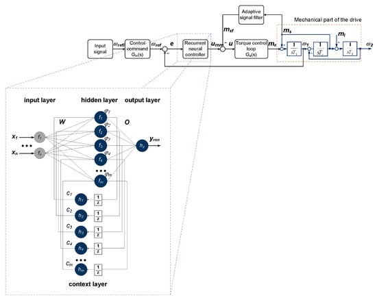
Figure 1.
The schematic diagram presenting the overall concept of the control structure.
The two-mass drive mechanical model is only a simplification of the real-life system [45]. The additional factors, such as the nonlinear characteristic of the mechanical connection (including mechanical hysteresis), the non-linear friction located on both sides, the imperfections in electromagnetically generated torque (for example, the torque ripples) and others, influence the control properties. All of these factors decrease the effectiveness of classical estimation techniques, which motivates the search for different techniques.
The reference speed (ωref) is the external signal that forces internal state variables and output speeds. For the proper (precise influence on the dynamic properties of the system) and stable work (without forcing dynamics higher than limits established through time constants of the plant) of the controller, an additional element at the input of the control structure was applied. It is defined by the following equation [3]:
where ω0 is the resonant frequency and the damping coefficient is noted as ξr.
A typical control structure most often consists of a cascade connection of two loops: the internal loop is used for electromagnetic torque control and the external loop is responsible for speed control. In the inner loop, the following elements can be distinguished: torque (current) controller, power converter and winding and current sensors. Usually, a PI-type controller is applied here. However, it should be stated that this controller is not robust. Changes of the system parameter(s) worsen the torque response, so a more advanced controller could be used, e.g., sliding-mode, fuzzy or predictive. On the other hand, the imperfect torque control can be treated as an additional unmodeled dynamic (disturbance) for an adaptive speed controller.
The representation of the current controller, power electronic devices and current sensors is possible by the expression shown below:
In this application, for most of the analyzed issues, the ideal electromagnetic torque control loop is assumed (the total time constant for current processing is Tme = 0 s). This means that delays in the mentioned part of the control structure are not taken into account. This assumption is possible (obviously for a limited range of forced dynamics) in modern electrical drives (fast processors used for data analysis and calculations, dynamic control of power systems, etc.).
The control signal, u, is defined as a combination of the neural part, urnn, and additional feedback from the shaft torque (attaching an additional signal related to the object enables more accurate damping of torsional vibrations [11]):
where msf is the filtered value of the shaft torque, ms.
The input of the neural controller is described by the following formula:
where ω1 is the value of the motor speed.
The signal msf is calculated using a special connection of neural models. Details of this part of the control structure are presented in the following sections.
The primary element of the adaptive controller is based on a recurrent neural network. In this application, the Elman model was implemented [46,47]. The output value of this model (yrnn) is used in (7):
where ku is the constant output gain.
The recurrent neural network realizes parallel data processing. A characteristic part of the calculations is the multiplication of input signals, for several layers and weights. In the considered neural controller, the following parameters describing the structure of the neural network were assumed (according to the notation used in Figure 1): two inputs (n = 2), five hidden nodes (m = 5) and one output (z = 1). Therefore, a mathematical equation for calculation of the output signal of a recurrent neural network is presented below:
where W[nxm] is the matrix between the inputs and the hidden layer, with elements wih, O[mxz] is the matrix between the hidden layer and the outputs with elements oh, C[mx1] is the matrix of weights for the context layer with parameters ch, h is the actual analyzed hidden node, i is the actual analyzed input and k is the sample number.
In the expression above, φh is the output of the h-th hidden neuron:
The general definitions of the activation functions are as follows:
and
where β is the scaling factor (β > 0, most often from the range (0,1)), and a is the argument of the function.
In this model of the recurrent network, the hidden nodes contain an additional input signal. It is the output value from the previous iteration φ(k − 1), which creates a virtual layer in the structure. Therefore, the value of inh (Equation (10)) is calculated using the following formula:
The input and output weights and scaling parameters for the context layer are adapted on-line (using matrix notation):
In the adaptation process, the gradient method was used, therefore the cost function was defined as follows:
where yref is the reference signal for the control structure and y is the output value.
Then, Equations (15)–(17) can be redefined as:
In Equation (21), μ is the learning coefficient.
Now, the partial derivatives have to be calculated using the chain rule:
In the above calculations, Equations (14) and (18) are used. Moreover, δ is defined by the expression:
The general structure of the adaptive controller includes one output and two inputs. Often, for those variables, additional scaling coefficients are provided, and one of them was presented in Formula (9). The following gains are: ke for control error and kde for derivative of speed error. The influence of these coefficients on the control precision and the proposed method of value determination is analyzed in Section 4 of this paper.
3. The ADALINE Model
3.1. Structure and Parameters’ Adaptation
The adaptive element analyzed in this section is the basis for the adaptive filter included in the control scheme (Figure 1). The extended considerations of ADALINE have been proposed in [48]. The operation of a single unit (with a linear function and threshold) as well as the connection into an extended network are presented. The overall concept of calculations is similar to the typical processing of a classical neuron. The input values are multiplied by the weights (here, bias was omitted), and the argument for the transfer function is the sum of all signals (in this case, the linear function, f, was used):
where ya is the output of the ADALINE model, xa is the input of the node, wa is the weight of input i and k is the number of iterations.
In this application, the adaptation of weights has been realized on-line:
Typically, the optimization of the weight matrix, Wa, is deduced from the analysis of the influence of the network coefficients on the cost function:
In the equation above, yaref is the reference signal for the node.
The training procedure should assume changes of weights that lead to the minimization of the error, Ea, in the subsequent steps of processing:
and using the expression (28):
Often, the state expansion in Taylor series is applied for the analysis of the cost function. After modifications, Equation (31) can be rewritten as:
With some approximation, one can write the equation:
The gradient determination can be carried out using the following calculations:
Equation (33) is achieved if:
Therefore:
Combining the above considerations, the basic equation defining the update of weights in the ADALINE model is obtained as:
In publications, normalization of the input vector is also suggested and used in real solutions [49,50]:
Subsequent calculations show the behavior of the algorithm (38) in the subsequent stages of training. The output signal, (26) and (27), can be described using matrix notations:
The reference value, yaref, is achieved at the output of ADALINE for optimal weights, Wao:
The precise definition of the error (34) can be represented as the following equation:
The weight error in the next iteration is expressed as follows:
Combining (41) and (42):
The equation presenting the changes of the error weight is formed:
Now, the discrete-time Lyapunov function, for stability analysis, is defined [51]:
For the proper work of the ADALINE training, the following conditions should be maintained:
Using the previous results in this section, the above formula has been written as:
Lower values of weight error in the following steps of training are obtained for:
The calculations presented above and the conclusion in the final inequality show the range of accepted values that can be applied for the α parameter. However, a certain level implemented in practical solutions can force the system to operate in different dynamics. A small number (α) in Equation (37) enables a more precise search for the optimal value of the weight matrix. However, it takes longer to search for the appropriate values. On the other hand, a high value of the training coefficient enables a quick jump towards the optimum. However, the precision of the calculations may not be very high. In engineering applications, it seems advantageous to introduce a variable value (high for large error—faster closing to minimum of the cost function, low for small error—more accurate calculations) for the coefficient α [21].
3.2. Concept of Neural Filtering
There are two general structures for neural filtering that are mainly considered in the papers. The first of them needs correct calculation information about the noise level or the reference signal. The learning procedure leads to the estimation of inaccuracies [52,53]. The second idea of adaptive neural filtering switches the reference signal to a historical sample of the disturbed waveform. In such a situation, the neural model is forced to calculate an improved transient. This strategy is often also called signal enhancement. However, both methods make it possible to obtain higher signal quality [53,54,55]. Low computational power necessary for the algorithm calculation should also be noted.
In this article, on-line tuning (presented in the previous section of the article) of the ADALINE model was applied for error minimization (ea). The difference between the reference, yaref, and the output, ya, signals was reduced. In this application, ADALINE with four inputs was used (Figure 2). The input state variable was the measured shaft torque, yaref = ms(k − 1). Subsequent inputs contain values from historical samples of previous input (unit delay elements were applied). The adaptive model should calculate the shaft torque, msf, with a lower level of noise. The training coefficient (α) was experimentally selected. Initial values of weights can be selected as random numbers or zeros.
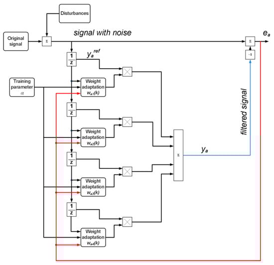
Figure 2.
Neural filter based on the ADALINE model.
This application is related to the electrical drive. The control structure, presented in Figure 1, assumes the connection of an additional feedback from the shaft torque. In many solutions, it is not measured directly. This signal is calculated using suitable observers or simple simulators based on equations. It should be noted that the basic information in the determination of the mentioned state variable is the current signal. It is often a disturbed waveform. The following calculations (using gains or derivative operations) can additionally amplify the disturbances. Moreover, the low-cost construction of the drive is expected. Thus, the implemented sensors may be characterized by a limited accuracy of processing. Additionally, it may not be possible to obtain a small calculation step using cheap programmable devices.
In order to present the properties of the separate part of the system from Figure 1 (the neural filter of shaft torque), simulation tests were carried out. The frequency of calculations was set to fs = 1000 Hz. For this purpose, a disturbance was introduced by adding the value from the random number generator (pseudorandom numbers from normal distribution) to the torque signal. Obviously, in the experimental tests, the ms would be msn. Exemplary results are presented in Figure 3. The learning coefficient was equal to 0.9. The original signal (black marker) and a disturbed transient are presented (red marker). Then, as the result, the output of the ADALINE filter is shown (green marker). The figures (for the same test) are presented twice. In the first case, the long-term drive reversions are presented (Figure 3a). The second graph shows an enlarged fragment of the processed state variable. The aim was to show the stable operation of the adaptive filter (the first case) and transients’ details (the second case). It is easy to notice a significant improvement in signal quality (Figure 3b). The convergence of the algorithm can also be observed. Another advantage of this type of filtering is the lack of delay in the processed signal.
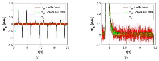
Figure 3.
Results of shaft torque processing using the ADALINE model (entire transient (a) and zoom (b)).
4. The Particle Swarm Optimizer Implemented for ke and ku Selection
The adaptive controller, based on a recurrent neural network, contains a reconfigurable part (weights updated according to the training rule). However, the overall structure includes the constant coefficients that need to be defined during the design stage. It is related to the gains applied for the input signals ke (error) and kde (error derivative) and the control value ku. The mentioned parameters are significant for the proper work of the control system. The validity of the assumptions presented above is verified in the results shown in Figure 4 and Figure 5. If the ke is small (ke = 1), the information about the speed control error is insufficient, and as a result, the correct operation of the controller is difficult to obtain. In the case of an overestimated value of this coefficient (ke = 50), the controller may react with too-rapid changes of the control signal. Then, oscillations appear under the load switching (Figure 4). There is a suitable (intermediate) gain value for the signal at this controller input. Similar dependencies can be observed in the transients of machine speed and load saved for other values of the ku parameter. It can force high-frequency oscillations of the state variables (ku = 50), but also a slow response of the plant (ku = 10). Correct selection of the control signal amplification ensures an appropriate reaction (according to the control signal) in the transient states of the drive operation. Analytical derivation of the formulas describing the fixed parameters of controllers based on artificial intelligence algorithms (neural networks or fuzzy logic) is difficult, and often these values are determined experimentally. One of the solutions for this problem is application of a nature-inspired algorithm. In this case, the particle swarm optimization method was used. Moreover, one of the assumptions, during the implementation of the main controller presented in Figure 1, was to reduce the parameters needed for selection at this stage. The analyzed results were performed for kde = 1. This means that it is possible to obtain an effective controller without insertion of this parameter. In further optimization, only ke and ku are considered.
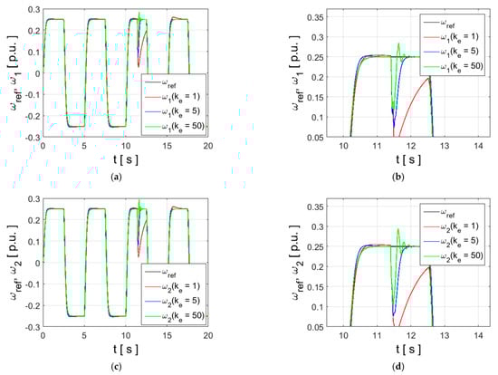
Figure 4.
Transients of motor (a,b) and load speed (c,d) in the control structure—influence of the input gain of the controller.
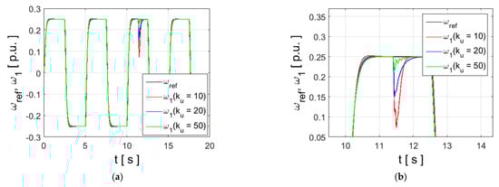
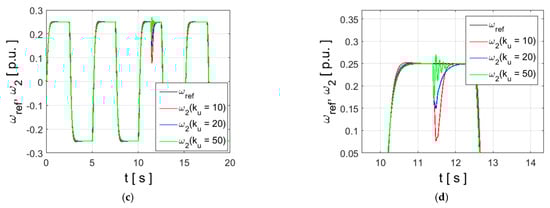
Figure 5.
Motor speed (a,b) and load speed (c,d) in electrical drive with elastic shaft—influence of the output parameter in the RNN controller.
The background of the calculations performed in the PSO is based on the group behavior of organisms. It is compared, in an article presenting the principles of the algorithm, to a flock of birds or the movement of a shoal of fish [56]. The group is considered as a set of potential solutions, among which appropriate values are searched, to find the optimal solution. The search for food is represented by the continuous update of individual parameters. For each element of the set, the characteristic parameters are assigned. These coefficients describe the position among other particles, and also affect the subsequent stages of calculations [57]. To specify, the most important factors describing the elements of the solution set are presented below.
The coefficients describing the accuracy for the next potential solution (for the k-th particle) are as follows: εkp is the value closest to the optimal level, and εkg is the state of the particle related to the global minimum of the cost function, defined as follows:
where:
n is the total number of samples, p is the analyzed sample, u is the control signal and a1 and a2 are design parameters.
The above-presented construction of the cost function contains (apart from the error of speed control, ω1, calculated on the basis of the signal from the motor) an additional component, whose task is to reduce oscillations in the control system. Besides, in this way, the algorithm prevents reaching extreme values of the controller parameters.
The following coefficient is the velocity of the particle νk in the i-th iteration, and is defined according to the formula:
where c1 and c2 are constant parameters (acceleration), typically selected in the range:
Moreover, in the formula describing the velocity, additional parameters (randomly selected) are used:
The last coefficient for the k-th particle is position:
In this implementation of the PSO, the modified version of Equation (54) was applied. The inertia weight, wpso, was inserted [58]:
Additionally, time-varying coefficients of the velocity equation were assumed:
where wpsomax and wpsomin are the upper and lower bounds of the wpso, i is the actual step of processing and imax is the maximal number of iterations.
The acceleration parameters c1 and c2 are recalculated for each iteration according to the expressions [59]:
where c1init is the initial value of c1, c1final is the final value of c1, c2init is the initial value of c2 and c2final is the final value of c2.
The impact of changes in the νk above, analyzed by the optimization process, are presented in [60].
The PSO algorithm performs data processing based on the mathematical relationships shown in the previous paragraph. The PSO algorithm is implemented in subsequent iterations. The basic computations are simple, they do not require the derivative of the objective functions with respect to the optimized parameters. At the initial stage, the data processing conditions are declared: the number of elements of the set, the maximum number of iterations, the limitations of the assigned parameters, the range of parameters described with Equations (59)–(61), etc. The initial values of the solution set are randomized. In order to initially evaluate the whole set, the error is calculated for each parameter (particles). Then, the repeating part of the algorithm is started. The coefficients used in the speed calculation are determined (wpso, c1 and c2). The main part of data processing, in the search for the optimum, is determining the speed and position for subsequent particles. After checking the quality of the obtained results, the criteria for stopping the calculations are analyzed. If the conditions are not met, the following iteration is realized. The following stages of calculation are presented in the diagram in Figure 6.
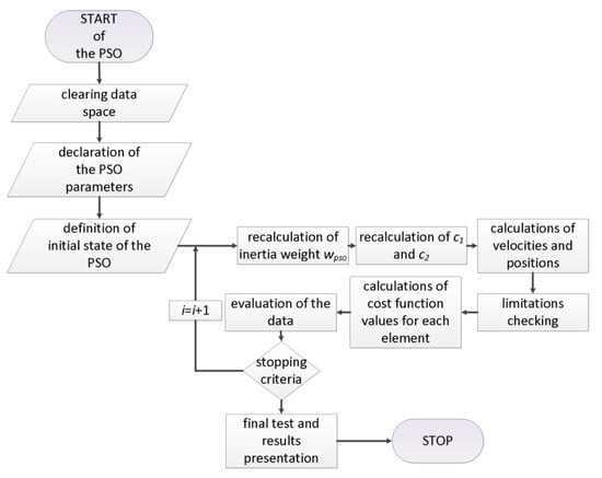
Figure 6.
The scheme presenting the overall concept of the PSO optimization.
As mentioned earlier, in this article, the purpose of the PSO algorithm is to determine the parameters of the adaptive neural controller that uses the recurrent model. In this application, for the acceleration factors, the following range was assumed: c1init = 2.5, c1final = 0.5 and c2init = 0.5, c2fina l = 2.5. The value of the wpso parameter was decreased from 0.9 to 0.1. For two calculated parameters (ke and ku), 20 individuals of the processed set of solutions were appointed. Data modifications were carried out over 30 cycles. The initial value of the objective function is very large (Figure 7a). This state corresponds to the drawn initial values (ke = 0.5688, ku = 2.5508). Transients of the ω2 speed are presented in Figure 7b. The mentioned controller parameters do not ensure stable operation of the control system (red marker). In the following calculation steps, the error values decrease (Figure 7a). As a result, the following values of gains for the controller were achieved: ke = 4.1058, ku = 23.6211. Optimized parameters lead to precise control of the drive. The obtained values were used in the tests of the control structure.
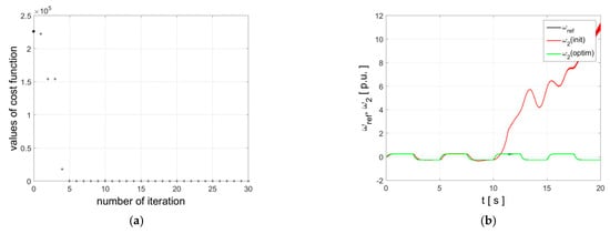
Figure 7.
Results of the PSO optimization—the objective function values during the calculations (a) and output signal (load speed) of the drive (b).
5. Simulations of the Control Structure
This stage of work focused on the numerical analysis of the control structure. Firstly, a simulation model was developed for the system. The following values of time constants were assumed for the object: T1 = T2 = 203 ms and Tc = 0.0012 s. The sampling time was set to ts = 0.0001 s. Several simulations take 30 s. The reference speed is not constant. Initially, this signal starts from 0 to 25% of the nominal value. Then, this transient was changed from the set value to −0.25. Subsequent sequences force the drive to the following reversals. All state variables were represented in the unit system. The drive is started with no load. At t = 11.4 nominal, the load was turned on.
The previous paragraph presents the general assumptions of the simulation tests. The state variables’ responses are shown in Figure 8. The aim of the first studies was to demonstrate the correct operation of the control system. Nominal values of the time constant were assumed. At the initial phase of the drive operation, control inaccuracy is visible (Figure 8a,b). It is related to the random initial values of the neural network coefficients. The neural elements of the control structure are adapted to carry out the relevant tasks (controller and filter). However, after a short period of time (about t = 1 s), the adaptive algorithm tunes the coefficients correctly, and as a result, the speeds (ω1 and ω2) of the drive follow the reference signal. It does not affect the stability of the system. The reaction of the system to load switching is very fast, and the speed returns to the set level after a short time. Obviously, it is related to the step of the current (electromagnetic torque, me). At the transient state, the me variable has higher values than the shaft torque (Figure 8c). Thus, proper operation of the drive can be achieved.
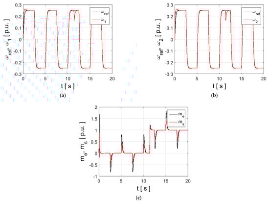
Figure 8.
Transients of state variables in control structure with adaptive neural controller applied for two-mass system—motor speed (a), load speed (b), shaft torque and electromagnetic torque (c).
Figure 9 and Figure 10 show operation of the electrical drive under disturbed time constants of the mechanical part. The parameters of the load (T2) and shaft (Tc) have been changed. Identical parameters of the regulator were introduced. Moreover, once drawn, weight values were loaded before the start of each calculation. In this way, appropriate values that make it possible to compare the performance of the speed controller under different operating conditions are provided. In these figures, the plots of the speed tracking present the high quality of the control. Several transients are close to the reference signal. For changes of the time constant, T2, different values of the electromagnetic torque are noticed in transient states. It is related to changes in the moment of inertia. It can be considered that an object with a larger time constant is heavier, so a higher current is required as the speed value changes. The simulated disturbances, introduced as changes of the shaft constant, in a real case may correspond to tests performed for couplings with different properties that result from the quality of the material or the diameter of the connection.
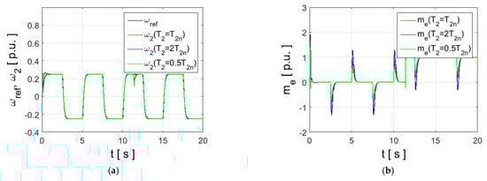
Figure 9.
Transients of state variables (load speed (a) and electromagnetic torque (b)) in control structure with adaptive neural controller applied for electrical drive with elastic coupling—changes of the mechanical time constant of the second motor.
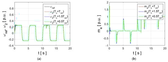
Figure 10.
Transients of state variables (load speed (a) and electromagnetic torque (b)) in control structure with adaptive neural controller applied for electrical drive with elastic coupling—changes of the shaft time constant.
The two-mass system, in this research, is represented as the mechanical part of the electrical drive. A flexible shaft creates a non-ideal connection that disturbs the waveforms of the state variables. This construction can cause oscillations that make precise speed control difficult. However, according to the mentioned assumptions, the current control loop is a delay for the outer loop with the RNN controller. Moreover, a two-mass system can be formed through an electrical drive with different types of machines. Considering the analyzed control structure, some versatility in the application and design process can be inferred. Therefore, the last simulation deals with the influence of Tme on the final results (Figure 11). It should be highlighted that it is a summary time constant, including current measurement, controller operation and power electronic devices. In previous tests, an ideal torque control loop was assumed (Tme = 0). The control system works very well in the studied range of Tme values. This is an additional advantage of the RNN controller. It also leads to the conclusion that the design process can be simplified.
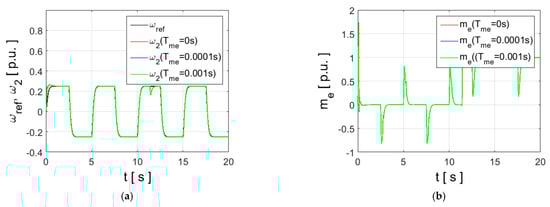
Figure 11.
Transients of speeds (a) and electromagnetic torque (b)—analysis of the processing time of the internal control loop.
6. Experiment
The proposed adaptive control structure has been examined in the laboratory ring. The main part of the experimental set-up consists of two converter-fed DC machines (500 W each) coupled by a flexible connection. Both electrical motors are controlled by a control card (dSpace 1103) via two separate power converters. The whole control algorithm is implemented with the help of this control card. In the realized control structure, two main control loops are visible, namely the torque and speed. The inner driving torque loop encompasses the following elements: PI torque controller, transistor H-bridge (power converter), armature winding and current sensor (LEM type). The current signal supplies a 16-bit A/D converter of the control card. The control signal of the reference current is transformed to a PWM signal and is sent to transistors of the H-bridge (with switching frequency of 10 kHz). The parameters of the current controller are set in order to obtain a fast torque response. In this application, the torque inner loop can be approximated by an equivalent first-order term with time constant equal to 1 ms. The outer speed control loop consists of a speed controller, optimized inner control loop, mechanical part of the drive and the incremental encoder fixed to a driving motor. The encoder’s signal is sent to the control card. In the experimental set-up, there is also a second encoder mounted to the load machine. However, it is not used for the control purpose but only to monitor the position of the load. The main data of motors are: nominal power PN—500 W, nominal speed nN—1450 rev/min, nominal current IN—3.15 A, nominal voltage UN—220 V and moment of inertia JN—0.0044 kg m2. In Figure 12, the sample layout photos are presented.
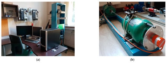
Figure 12.
Experimental set-up—power electronics (a) and electrical machines (b).
The conducted research took into account the assumptions typical for this stage of research related to the electric drive control system, which means issues related to the selection of a programmable device and the method of algorithm implementation. As it was mentioned above, the dSpace 1103 card was used in the laboratory. It is a powerful tool with enough computational power needed for control algorithm implementation. The neural network with on-line weight adaptation was initially implemented in a high-level graphical programming language. The above-described assumptions are commonly known in academic or research centers’ methods. Firstly, the design process is focused on the overall idea, then technical problems are performed. However, two development scenarios are considered in the following work. The first of them deals with the low-cost implementation of the control algorithm. On the other hand, due to the parallel data processing (in the main controller and adaptive filters), the field programmable gates arrays can be used. To improve the efficiency of the code (higher frequency of calculations), the analyzed speed controller can be implemented using the low-level programming technique. The control software (settings of reference values, graphical data representation, etc.) can be prepared, as a standalone application, using Python with graphical libraries.
A number of experiments have been carried out to test the performance of the analyzed control structure with an adaptive controller. The parameters of the input filters are as follows: ωn = 20 s−1 and ξr = 1. The drive is working under the following cycle: the reference command of the motor speed is changing from −0.25 to 0.25, with frequency of 0.2 Hz. The speed reference, taken as 25% of the nominal level, makes it possible to prevent the control system from operating within current limits. In this way, the operation of the control system and the properties of the controller can be clearly observed without the additional influence of disturbing elements. In control theory, the limitation of the control signal is a separate issue. Additionally, this assumption is used for comparative reasons (with other types of controllers). This is also beneficial for the safe operation of the drive during the initial tests. The shape of the reference signal deals with repetitive industrial processes (e.g., work of a robot used in a production line). Moreover, this trajectory is proper for tests of adaptive systems. Through repeated actions, it is possible to observe the reduction of the control error. Additionally, the longer working time presented in the speed transients can be considered as a practical verification of stability.
In the first case, the system is working without external load. Transients of the working system are presented in the following order: motor and load speeds (Figure 13a) and electromagnetic and shaft torque (Figure 13b). Next, the system with a changeable load torque is tested. The disturbance is switched on and off after 1 and 2 s of negative reversal.
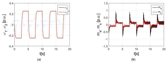
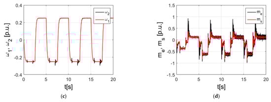
Figure 13.
Transients of state variables in the control structure with an adaptive neural controller applied for the two-mass system—motor speed (a,c), load speed (a,c) and shaft torque and electromagnetic torque (b,d).
As can be concluded from the transients presented in Figure 13, the drive system is working correctly. Both speeds follow the reference command precisely without visible errors (Figure 13a,c). The changing of the reference signal creates the transient state, yet during this time, errors in both speeds are not noticeable. The transients of both torques possess noises, yet they are smaller for the shaft torque. The switch on and off of the load torque creates small, quickly damped oscillation in the load speed, yet the motor speed remains almost constant (Figure 13c). Those small oscillations are also visible in electromagnetic and shaft torque transients (Figure 13d).
The proposed system can be implemented into two ways: without and with additional feedback from the shaft torque. The above consideration can be significant in real industrial applications. Introducing additional information from feedback improves the damping of torsional vibrations. Therefore, higher precision of work can be achieved. However, next, sensors are needed, which leads to higher costs and increased susceptibility to faults. Concluding the above, it can be a compromise that depends on the specific facility and system requirements.
In order to show the advantage of the second approach, the following experimental tests were performed. Firstly, the system without this feedback is implemented, then it is added to the control structure. The drive is working under the following cycle: the reference signal of the speed is set to 0.1, with a frequency of 0.2 Hz. No external load torque is applied to the system this time. The obtained transients for the structure without and with additional feedback are shown in Figure 14.
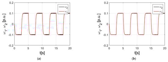
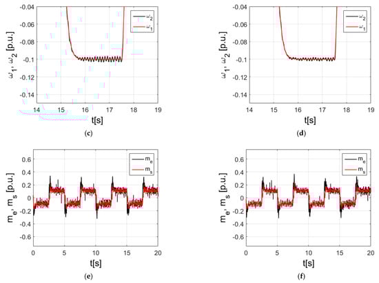
Figure 14.
Transients of state variables in the control structure with an adaptive neural controller applied for the two-mass system—motor speed (a,b), fragment of speeds (c,d) and shaft torque and electromagnetic torque (e,f) for the control structure without (a,c,e) and with (b,d,f) additional feedback from the shaft torque.
Both tested systems work correctly. The speeds follow signals with small errors (Figure 14a,b). The difference between both systems is visible at the enlarged plots of the speeds (Figure 14c,d). The control structure with additional feedbacks from the shaft torque allows to suppress oscillations of the load speeds much more effectively. These oscillations have about a 50% smaller magnitude than in the control structure without additional feedbacks. The transients of electromagnetic and shaft torque are presented in Figure 14e,f. Due to the high level of noises, there are no visible differences between these control structures.
Then, the effectiveness of the time-processing system was tested in an experimental study. The system works in an identical cycle as that used previously. The obtained transients are shown in Figure 15.
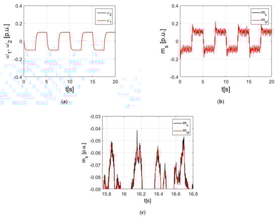
Figure 15.
Transients of state variables in the control structure with an adaptive neural controller applied for the two-mass system—motor speed and load speed (a), real and filtered shaft torque (b,c).
In the control system working under reverse condition, both speeds follow the reference command without noticeable errors. The torques of the system are presented in Figure 15b and its enlargement in Figure 15c. It is clearly seen from the last figure that the filtered shaft torque possesses a lower noise level. Due to the adaptation algorithm applied for the simplified neural model, a reduction of disturbances can be achieved without a complex algorithm or a complicated design process. Additional output delays are not observed. However, besides the overall level of noise, the elimination of the short-peak points (Figure 15c, about t = 16.1 s) is also very important for the control structure. In the closed control loop, it can be amplified. Then, it can be reflected in the snatch of the shaft between the motors. It can be a source of the faults in the mechanical part of the drive.
7. Conclusions
In this paper, we presented issues related to the application of the adaptive neural controller for the drive system with an elastic shaft. The neural system is based on the recurrent architecture and it was tuned on-line in order to minimize the control error. In order to ensure the better damping ability, we included the additional feedbacks from the shaft torque to the control structure. The noises existing in the signal of the shaft torque were suppressed by the ADALINE system. The features of the considered drive system were illustrated by the simulation and experimental results. Based on the theoretical considerations as well as the simulation and experimental tests, we can formulate the following concluding remarks, as presented below.
- In order to suppress torsional vibrations of the two-mass system with changeable parameters (or unknown), there is a need to apply an advanced adaptive control structure. The proposed recurrent neural controller allowed to effectively dampen the torsional vibration, and also, in the drive, possessed additional non-inebrieties such as friction or a nonlinear mechanical shaft (evident in real drives).
- The properties of the control structure depend on input (ke, kde) and output (ku) coefficients. The correct selection of those values is not a trivial task and depends on particular parameters (or their range) of the plant, cycle of work and additional nonlinearities. The proper work of the control structure can be achieved by suitable selection of two of the above-mentioned parameters. In this work, the coefficients ke and ku were selected with the help of the particle swarm optimization method. This algorithm allows to obtain the optimal value to specify the cost function, which resulted in optimal damping ability of the considered control structure.
- The damping ability of the adaptive recurrent controller can be increased by additional feedback from the shaft torque. However, in practical application, this signal can possess a relatively high noise level. In order to minimize the noise levels in the shaft torque signal, the ADALINE system was proposed. It allows to filter the shaft torque signal, which results in correct operation of the drive.
- The proposed control structure allowed to dampen the torsional vibration in the case of changeable parameters of the plant, such as time constant of load machine, stiffness time constant or different values of delay in the torque control loop. For all mentioned scenarios, speed oscillations were suppressed.
Author Contributions
Main idea, M.K. and K.S.; methodology, M.K. and K.S.; simulations, M.K.; validation, K.S.; formal analysis, K.S.; experiment, M.K.; analysis of results, K.S. All authors have read and agreed to the published version of the manuscript.
Funding
This research was supported by basic research funds of the Department of Electrical Machines, Drives and Measurements of the Wroclaw University of Science and Technology (2021).
Data Availability Statement
Not applicable.
Conflicts of Interest
The authors declare no conflict of interest.
Abbreviations
The main nomenclature assumed for presentation of theory and results are presented.
| Abbreviations: | |
| RNN | Recurrent neural network |
| PSO | Particle swarm optimizer |
| ADALINE | Adaptive linear neuron |
| ASD | Adjustable speed drive |
| FOC | Field-oriented control |
| MPC | Model predictive control |
| Parameters: | |
| T1 | mechanical time constant of the motor |
| T2 | mechanical time constant of the load |
| Tc | stiffness time constant |
| ω0 | resonant frequency |
| ξr | damping coefficient |
| Tme | total time constant for current processing |
| W | matrix between the inputs and the hidden layer |
| O | matrix between the hidden layer and the outputs |
| C | matrix of weights in the context layer |
| α | training constant |
| ke | input gain of the RNN (error input) |
| kde | input gain of the RNN (input with derivative of error) |
| ku | output gain of the RNN |
| ts | sampling time |
| State variables: | |
| me | electromagnetic torque |
| ms | torsional torque |
| msf | filtered value of the shaft torque |
| mL | load torque |
| ω1 | motor speed |
| ω2 | load speed |
| ωref | reference speed |
References
- Finch, J.W.; Giaouris, D. Controlled AC Electrical Drives. IEEE Trans. Ind. Electron. 2008, 55, 481–491. [Google Scholar] [CrossRef]
- Pimkumwong, N.; Wang, M.-S. Online Speed Estimation Using Artificial Neural Network for Speed Sensorless Direct Torque Control of Induction Motor based on Constant V/F Control Technique. Energies 2018, 11, 2176. [Google Scholar] [CrossRef]
- Orlowska-Kowalska, T.; Szabat, K. Control of the drive system with stiff and elastic couplings using adaptive neuro-fuzzy approach. IEEE Trans. Ind. Electron. 2007, 54, 228–240. [Google Scholar] [CrossRef]
- Zaihidee, F.M.; Mekhilef, S.; Mubin, M. Robust Speed Control of PMSM Using Sliding Mode Control (SMC)—A Review. Energies 2019, 12, 1669. [Google Scholar] [CrossRef]
- Brock, S.; Luczak, D.; Nowopolski, K.; Pajchrowski, T.; Zawirski, K. Two Approaches to Speed Control for Multi-Mass System With Variable Mechanical Parameters. IEEE Trans. Ind. Electron. 2016, 64, 3338–3347. [Google Scholar] [CrossRef]
- Luczak, D.; Wojcik, A. The study of neural estimator structure influence on the estimation quality of selected state variables of the complex mechanical part of electrical drive. In Proceedings of the 2017 19th European Conference on Power Electronics and Applications (EPE’17 ECCE Europe), Warsaw, Poland, 11–14 September 2017; pp. 1–10. [Google Scholar]
- Inoue, Y.; Katsura, S. Spatial Disturbance Suppression of a Flexible System Based on Wave Model. IEEJ J. Ind. Appl. 2018, 7, 236–243. [Google Scholar] [CrossRef]
- Xiang, B.; Wong, W. Electromagnetic vibration absorber for torsional vibration in high speed rotational machine. Mech. Syst. Signal. Process. 2020, 140, 106639. [Google Scholar] [CrossRef]
- Zhang, G.; Furusho, J. Speed control of two- inertia system by PI/PID control. IEEE Trans. Ind. Electron. 2000, 47, 603–609. [Google Scholar] [CrossRef]
- Goubej, M. Fundamental performance limitations in PID controlled elastic two-mass systems. In Proceedings of the 2016 IEEE International Conference on Advanced Intelligent Mechatronics (AIM), Banff, AB, Canada, 12–15 July 2016; pp. 828–833. [Google Scholar]
- Szabat, K.; Orlowska-Kowalska, T. Vibration suppression in two-mass drive system using PI speed controller and addition-al feedbacks—Comparative study. IEEE Trans. Ind. Electron. 2007, 54, 1193–1206. [Google Scholar] [CrossRef]
- Szczepanski, R.; Kaminski, M.; Tarczewski, T. Auto-Tuning Process of State Feedback Speed Controller Applied for Two-Mass System. Energies 2020, 13, 3067. [Google Scholar] [CrossRef]
- Saarakkala, S.E.; Hinkkanen, M. State-space speed control of two-mass mechanical systems: Analytical tuning and experi-mental evaluation. IEEE Trans. Ind. Electron. 2014, 50, 3428–3437. [Google Scholar] [CrossRef]
- Dodds, S.J.; Szabat, K. Forced dynamic control of electric drives with vibration modes in the mechanical load. In Proceedings of the 2006 12th International Power Electronics and Motion Control Conference, Portoroz, Slovenia, 30 August–1 September 2006; pp. 1245–1250. [Google Scholar]
- Serkies, P.; Szabat, K. Effective damping of the torsional vibrations of the drive system with an elastic joint based on the forced dynamic control algorithms. J. Vib. Control 2019, 25, 2225–2236. [Google Scholar] [CrossRef]
- Ohnishi, K.; Katsura, S.; Shimono, T. Motion Control for Real-World Haptics. IEEE Ind. Electron. Mag. 2010, 4, 16–19. [Google Scholar] [CrossRef]
- Katsura, S.; Suzuki, J.; Ohnishi, K. Pushing operation by flexible manipulator taking environmental information into ac-count. IEEE Trans. Ind. Electron. 2006, 53, 1688–1697. [Google Scholar] [CrossRef]
- Yamada, S.; Fujimoto, H. Precise Joint Torque Control Method for Two-inertia System with Backlash Using Load-side Encoder. IEEJ J. Ind. Appl. 2019, 8, 75–83. [Google Scholar] [CrossRef]
- Szabat, K.; Wróbel, K.; Dróżdż, K.; Janiszewski, D.; Pajchrowski, T.; Wójcik, A. A fuzzy unscented Kalman filter in the adap-tive control system of a drive system with a flexible joint. Energies 2020, 13, 2056. [Google Scholar] [CrossRef]
- Derugo, P.; Szabat, K. Adaptive neuro-fuzzy PID controller for nonlinear drive system. COMPEL Int. J. Comput. Math. Electr. Electron. Eng. 2015, 34, 792–807. [Google Scholar] [CrossRef]
- Kaminski, M.; Orlowska-Kowalska, T. Adaptive neural speed controllers applied for a drive system with an elastic mechanical coupling—A comparative study. Eng. Appl. Artif. Intell. 2015, 45, 152–167. [Google Scholar] [CrossRef]
- Amirkhani, S.; Mobayen, S.; Iliaee, N.; Boubaker, O.; Hosseinnia, S.H. Fast terminal sliding mode tracking control of non-linear uncertain mass–spring system with experimental verifications. Int. J. Adv. Robot. Syst. 2019, 16, 1–10. [Google Scholar] [CrossRef]
- Serkies, P.J.; Szabat, K. Application of the MPC to the Position Control of the Two-Mass Drive System. IEEE Trans. Ind. Electron. 2012, 60, 3679–3688. [Google Scholar] [CrossRef]
- Cychowski, M.T.; Szabat, K. Efficient real-time model predictive control of the drive system with elastic transmission. IET Control Theory Appl. 2010, 4, 37–49. [Google Scholar] [CrossRef]
- Gaidi, A.; Lehouche, H.; Belkacemi, S.; Tahraoui, S.; Loucif, M.; Guenounou, O. Adaptive backstepping control of wind turbine two mass model. In Proceedings of the 2017 6th International Conference on Systems and Control (ICSC), Batna, Algeria, 7–9 May 2017; pp. 168–172. [Google Scholar]
- Huang, Y.; Zhang, Z.; Huang, W.; Chen, S. DC-Link Voltage Regulation for Wind Power System by Complementary Sliding Mode Control. IEEE Access 2019, 7, 22773–22780. [Google Scholar] [CrossRef]
- Bo, T.X.; Phuong, T.T.; Ohishi, K.; Yokokura, Y.; Miyazaki, T. Robust position control using double disturbance observers based state feedback for two mass system. In Proceedings of the IECON 2016—42nd Annual Conference of the IEEE Industrial Electronics Society, Florence, Italy, 23–26 October 2016; pp. 5814–5819. [Google Scholar]
- Yokoyama, M.; Oboe, R.; Shimono, T. Robustness Analysis of Two-Mass System Control Using Acceleration-Aided Kalman Filter. In Proceedings of the IECON 2018—44th Annual Conference of the IEEE Industrial Electronics Society, Washington, DC, USA, 21–23 October 2018; pp. 4600–4605. [Google Scholar]
- Kaminski, M. Adaptive Gradient-Based Luenberger Observer Implemented for Electric Drive with Elastic Joint. In Proceedings of the 2018 23rd International Conference on Methods & Models in Automation & Robotics (MMAR), Miedzyzdroje, Poland, 27–30 August 2018; pp. 53–58. [Google Scholar]
- Tsai, C.-C.; Huang, H.-C.; Lin, S.-C. Adaptive Neural Network Control of a Self-Balancing Two-Wheeled Scooter. IEEE Trans. Ind. Electron. 2010, 57, 1420–1428. [Google Scholar] [CrossRef]
- Ebbesen, S.; Salazar, M.; Elbert, P.; Bussi, C.; Onder, C.H. Time-optimal Control Strategies for a Hybrid Electric Race Car. IEEE Trans. Control Syst. Technol. 2018, 26, 233–247. [Google Scholar] [CrossRef]
- Wang, Q.; Rajashekara, K.; Jia, Y.; Sun, J. A Real-Time Vibration Suppression Strategy in Electric Vehicles. IEEE Trans. Veh. Technol. 2017, 66, 7722–7729. [Google Scholar] [CrossRef]
- Ding, X.; Wang, Z.; Zhang, L.; Wang, C. Longitudinal vehicle speed estimation for four-wheel-independently-actuated electric vehicles based on multi-sensor fusion. IEEE Trans. Veh. Technol. 2020, 69, 12797–12806. [Google Scholar] [CrossRef]
- Ding, X.; Wang, Z.; Zhang, L. Hybrid Control-Based Acceleration Slip Regulation for Four-Wheel-Independently-Actuated Electric Vehicles. IEEE Trans. Transp. Electrif. 2021, 1. [Google Scholar] [CrossRef]
- Hunter, D.; Yu, H.; Pukish, M.S.; Kolbusz, J.; Wilamowski, B.M. Selection of proper neural network sizes and architectures—A comparative study. IEEE Trans. Ind. Inform. 2012, 8, 228–240. [Google Scholar] [CrossRef]
- Lin, F.-J.; Chen, S.-G.; Li, S.; Chou, H.-T.; Lin, J.-R. Online autotuning technique for IPMSM servo drive by intelligent identification of moment of inertia. IEEE Trans. Ind. Inform. 2020, 16, 7579–7590. [Google Scholar] [CrossRef]
- Li, S.; Won, H.; Fu, X.; Fairbank, M.; Wunsch, D.C.; Alonso, E. Neural-Network Vector Controller for Permanent-Magnet Synchronous Motor Drives: Simulated and Hardware-Validated Results. IEEE Trans. Cybern. 2019, 50, 3218–3230. [Google Scholar] [CrossRef]
- Gadoue, S.M.; Giaouris, D.; Finch, J.W. Sensorless control of induction motor drives at very low and zero speeds using neural network flux observers. IEEE Trans. Ind. Electron. 2009, 56, 3029–3039. [Google Scholar] [CrossRef]
- Kharat, P.A.; Dudul, S. Clinical decision support system based on Jordan/Elman neural networks. In Proceedings of the 2011 IEEE Recent Advances in Intelligent Computational Systems, Trivandrum, India, 22–24 September 2011. [Google Scholar] [CrossRef]
- Jordan, M.I. Attractor dynamics and parallelism in a connectionist sequential machine. In Proceedings of the 8th Annual Conference of the Cognitive Science Society; Erlbaum: Hillsdale, NJ, USA, 1986; pp. 531–546. [Google Scholar]
- Elman, J.L. Finding structure in time. Cogn. Sci. 1990, 14, 179–211. [Google Scholar] [CrossRef]
- Accetta, A.; Cirrincione, M.; Pucci, M.; Vitale, G. Sensorless control of PMSM fractional horsepower drives by signal injection and neural adaptive-band filtering. IEEE Trans. Ind. Electron. 2012, 59, 1355–1366. [Google Scholar] [CrossRef]
- Wang, L.; Zhu, Z.Q.; Bin, H.; Gong, L. A Commutation Error Compensation Strategy for High-Speed Brushless DC Drive Based on Adaline Filter. IEEE Trans. Ind. Electron. 2021, 68, 3728–3738. [Google Scholar] [CrossRef]
- Zhang, G.; Wang, G.; Xu, D.; Zhao, N. ADALINE-Network-Based PLL for Position Sensorless Interior Permanent Magnet Synchronous Motor Drives. IEEE Trans. Power Electron. 2016, 31, 1450–1460. [Google Scholar] [CrossRef]
- Bucolo, M.; Buscarino, A.; Famoso, C.; Fortuna, L.; Frasca, M. Control of imperfect dynamical systems. Nonlinear Dyn. 2019, 98, 2989–2999. [Google Scholar] [CrossRef]
- Lin, F.-J.; Shieh, H.-J.; Teng, L.-T.; Shieh, P.-H. Hybrid controller with recurrent neural network for magnetic levitation system. IEEE Trans. Magn. 2005, 41, 2260–2269. [Google Scholar]
- Ren, G.; Cao, Y.; Wen, S.; Huang, T.; Zeng, Z. A modified Elman neural network with a new learning rate scheme. Neurocomputing 2018, 286, 11–18. [Google Scholar] [CrossRef]
- Widrow, B.; Lehr, M. 30 years of adaptive neural networks: Perceptron, Madaline, and backpropagation. Proc. IEEE 1990, 78, 1415–1442. [Google Scholar] [CrossRef]
- Wang, Z.-Q.; Manry, M.T.; Schiano, J.L. LMS learning algorithms: Misconceptions and new results on convergence. IEEE Trans. Neural Netw. 2000, 11, 47–56. [Google Scholar] [CrossRef]
- Jannati, M.; Hosseinian, S.; Vahidi, B.; Li, G. Mitigation of windfarm power fluctuation by adaptive linear neuron-based power tracking method with flexible learning rate. IET Renew. Power Gener. 2014, 8, 659–669. [Google Scholar] [CrossRef]
- Man, Z.; Wu, H.R.; Liu, S.; Yu, X. A new adaptive backpropagation algorithm based on Lyapunov stability theory for neural networks. IEEE Trans. Neural Netw. 2006, 17, 1580–1591. [Google Scholar] [CrossRef]
- Widrow, B.; Lehr, M.; Beaufays, F.; Wan, E.; Bileillo, M. Learning algorithms for adaptive processing and control. In Proceedings of the IEEE International Conference on Neural Networks, San Francisco, CA, USA, 28 March–1 April 1993. [Google Scholar]
- Selvan, S.; Srinivasan, R. Removal of ocular artifacts from EEG using an efficient neural network based adaptive filtering technique. IEEE Signal Process. Lett. 1999, 6, 330–332. [Google Scholar] [CrossRef]
- Jindapetch, N.; Chewae, S.; Phukpattaranont, P. FPGA implementations of an ADALINE adaptive filter for power-line noise cancellation in surface electromyography signals. Measurement 2012, 45, 405–414. [Google Scholar] [CrossRef]
- Martinek, R.; Vanus, J.; Bilik, P.; Stratil, T.; Zidek, J. An efficient control method of shunt active power filter using ADALINE. IFAC-PapersOnLine 2016, 49, 352–357. [Google Scholar] [CrossRef]
- Kennedy, J.; Eberhart, R. Particle swarm optimization. In Proceedings of the ICNN’95—International Conference on Neural Networks, Perth, WA, Australia, 27 November–1 December 1995; Volume 4, pp. 1942–1948. [Google Scholar]
- Poli, R.; Kennedy, J.; Blackwell, T. Particle swarm optimization: An overview. Swarm Intell. 2007, 1, 33–57. [Google Scholar] [CrossRef]
- Marini, F.; Walczak, B. Particle swarm optimization (PSO). A tutorial. Chemom. Intell. Lab. Syst. 2015, 149, 153–165. [Google Scholar] [CrossRef]
- Ratnaweera, A.; Halgamuge, S.K.; Watson, H.C. Self-organizing hierarchical particle swarm optimizer with time-varying acceleration coefficients. IEEE Trans. Evolut. Comput. 2004, 8, 240–255. [Google Scholar] [CrossRef]
- Kaminski, M. Neural network training using particle swarm optimization—A case study. In Proceedings of the 2019 24th International Conference on Methods and Models in Automation and Robotics (MMAR), Miedzyzdroje, Poland, 26–29 August 2019; pp. 115–120. [Google Scholar]
Publisher’s Note: MDPI stays neutral with regard to jurisdictional claims in published maps and institutional affiliations. |
© 2021 by the authors. Licensee MDPI, Basel, Switzerland. This article is an open access article distributed under the terms and conditions of the Creative Commons Attribution (CC BY) license (https://creativecommons.org/licenses/by/4.0/).