Regional Diversity of Technical Efficiency in Agriculture as a Results of an Overinvestment: A Case Study from Poland

Abstract

Ensuring adequate profitability of production, which can be ensured by optimal investments, can encourage farmers to be more caring about sustainable development. Several existing studies indicate that technical efficiency in agriculture varies regionally. Investments comprise a basic way to increase efficiency and thus reduce polarisation between regions. However, contrary to established assumptions, not every investment leads to increased efficiency, which entails a phenomenon of overinvestment. Investments should, by definition, be positively correlated with efficiency. However, existing studies indicate the existence of a significant problem of overinvestment, where increased efficiency may not occur. While for about 40% of farms in Poland the scale of investments can be assessed as optimal, more than quarter of farms exhibited absolute overinvestment and nearly one in five farms is underinvested. In response to this problem, this study aimed to identify regional differences in Poland with regard to overinvestment in farms, as well as to determine changes in farm efficiency depending on the region and level of overinvestment. The source material used in the following article consisted of unpublished Farm Accountancy Data Network (FADN) microdata derived from the DG AGRI of the European Commission. The study covered the period 2004–2015. For an original classification of farms according to their level of overinvestment the technical efficiency, using the stochastic frontier analysis approach, was used for determining regional differences that occurred as a result of overinvestment. Stochastic frontier analysis shown noticeable differences in the average technical efficiency for different overinvestment groups. As expected, underinvested farms are the least efficient (general in Poland and in all analyzed regions) and average technical efficiency did not increase. Interestingly, optimally investing farms do not have the highest technical efficiency. Higher efficiency was achieved by both relatively and absolutely overinvested farms. This is due to the fact that in order to produce efficiently in agriculture, it is necessary to at least maintain the level of tangible assets provision, and preferably to increase it as well. In terms of overinvestment levels, farm structure does not differ significantly between individual regions in Poland. However, there are differences between regions in terms of farm efficiency within each group. In all regions, only the underinvested farms did not increase their efficiency over the period under review and the highest efficiency growth rate was in regions where farms were least efficient at baseline.

1. Introduction

Regionalism accompanies every aspect of economic and social development, and the diversity of regional development has a historical, climatic and cultural basis. Such diversity also appears in the context of agricultural investments and may be observed at the level of continents, states or regions of individual countries.

This study aimed to identify regional differences in Poland in terms of overinvestment in farms, as well as to determine changes in farm efficiency depending on the region and level of overinvestment. The research was based on individual farm data collected under the European farm accountancy data collection system FADN. The study covers the period 2004–2015, as this was a time of increased investment in Polish farms, and certain studies [1] reported that structural funds available under the Common Agricultural Policy (CAP) constituted an investment incentive for farms. The research covered Polish farms that continuously participated in the agricultural accounting system FADN during the examined period, which ultimately resulted in 3964 farms being included in the analysis. The study was conducted in accordance with the FADN regional division.

The following study is a contribution to the literature in that it identifies regional differences in farm efficiency depending on the level of overinvestment. The research was designed to answer the following questions: Is there any difference in farm structure depending on the level of overinvestment among individual regions? Are there any differences in farm efficiency between the regions in individual groups? Did the technical efficiency of farms increase during the period under review? To answer these questions, the authors used a novel and original classification of farms according to the level of overinvestment using the stochastic frontier approach.

The paper is organised as follows: in the Section 2, the authors describe the unique FADN source data and applied research methods; in the Section 3, the most significant research results are presented and discussed. Section 4 includes a summary and conclusions, as well as some indications concerning future studies.

2. Literature Review

There is an increasing acknowledgement that the spatial context of a farm’s location has a significant influence on the farmers’ strategic behaviour [2] and that differences in capital market structures across the countries alter investment sensitivity and affect agricultural competitiveness [3]. Regional policy creation can diversify investments, since farm investments are positively associated with public programmes providing support in the form of subsidies [4]. A study conducted by Manevska-Tasevska et al. [5] concerning the diversity of regional efficiency in the Swedish agricultural sector revealed that labour input, the value of owned assets and production differences were the most diversified elements among the regions under study. In Romania, research on regional diversity in agriculture has demonstrated that, due to irrational political decisions, the analysed regions varied in terms of technical capital owned, whereas low investments, issues arising from land ownership and ageing population contributed to the widening of regional differences in agricultural productivity and competitiveness [6].

In Poland, such diversity is sometimes distinguished at the level of self-government units, e.g., voivodeships. Diversification of agricultural investments includes the aforementioned bases (historical, climatic and cultural), differences in plant or animal production and income stratification, in addition to agrarian and production concentrations in different regions. The problem of disproportional investment expenditures in agriculture is visible in the regional diversification of Poland [7].

Investment may be interpreted as the involvement of the funds saved. These funds comprise a certain amount of money and capital expenditures on expenses related to the purchase of new goods or means of production, which, as a result, may improve work, multiply income, positively affect work security or fulfil the needs of society [8,9,10,11,12]. Investments aim to provide the investor with a return on the outlays invested in particular projects in the future (revenue), which will compensate for the period in which the money was invested. Inflation rate and investment risk [13,14] are integral components of economic activity [15], and investments are also factors contributing to the creation of rapid economic growth [16], and simultaneously, its effects. The basic aim of investments is to increase income, production and the quality of manufactured products, improve work safety [17,18,19], introduce new technologies, diversify agricultural activity and adapt agricultural production to the requirements of environmental protection [20]. Additionally, market units may decide to undertake risky and often more capital-intensive investments, as these increase the likelihood of higher returns and determine the product quality [21].

Agriculture is a fundamental branch of any economy, as it provides food security [22] through cultivation and breeding [23]. Agricultural development is necessary to maintain a safe level of nutrition amid an ever-increasing world population, which is estimated to reach 9.7 billion in 2050 [24]. The principal function and task for agriculture is to provide adequate quantity and quality of food that is necessary for the development of the population, while protecting natural resources in the same time, by means of using it in a sustainable way [25]. The sustainability of agriculture on the macro scale (sectoral level) can be achieved by improving sustainability on the micro level i.e., on the farms [26]. It consists of obtaining stable, and at the same time, economically and socially acceptable production in a way that does not threaten the natural environment. Achieving a high degree of sustainability of farms relies on economic sustainability. The economic dimension of sustainability is reflected, inter alia, in investments, which stimulated by an economic effect have a direct or indirect positive impact on environmental sustainability. Ensuring adequate profitability of production can encourage farmers to be more environmentally conscious considering environmentally sensitive natural resources as the foundation of the farm business. Farms that efficiently convert inputs into outputs will be able to meet this challenge. For these reasons the sustainable development of the agricultural sector is supported by intervention instruments in many countries.

Investment in agriculture is important for financial reasons [27], as is production growth, which in turn determines the release of resources to other sectors of the economy, and thus constitutes the foundation for efficient industrialisation [28], in addition to improvement of farms’ operational quality [29] and enabling food security that is consistent with the principles of environmental sustainability [30]. A lack of investment in farms may consequently lead to lower productivity [31,32], whereas improvement of farm performance through investment may increase its productivity [33]. Investments that aim to increase agricultural productivity are estimated to balance the adverse impact of climate change and thus reduce the number of people at risk of hunger [34]. Furthermore, agricultural investments reduce poverty and provide environmental protection [35,36], and they also foster development of the entire agricultural industry [16]. Investment projects aim to substitute living labour with capital, which is a consequence of changes in production factor prices, among which labour costs exhibit the highest dynamics [37]. The production investments undertaken constitute a determinant of opportunities for farm development. They indicate that the farmer is increasing the stocks of tangible assets or improving their quality, which is expected to increase the farm’s potential in the future. Improvements in the technical means of labour and the introduction of advanced machinery and equipment into agricultural production lead to increased productivity of both plant and animal production [38]. Modern agriculture requires the involvement of capital, but not all agricultural, high-risk investments have to bring profit in the short term [39], since they may be directed towards a long-term achievement of sustainability in all its dimensions (including social and environmental) [40]. In agriculture, it takes a certain amount of time before the contributed capital provides a return on investments or before the increased productivity results in efficiency [41]. Moreover, unplanned but necessary investments frequently need to be covered with credit funds, which are not equally accessible in all countries. For example, in a country such as Pakistan, the economy is based on agriculture, but it simultaneously has such high credit restrictions that the development of agriculture is consequently inhibited [42]. Therefore, there are areas in which overinvestment is a problem and areas where it is a lack of investment that causes improper functioning of the sector.

However, from the perspective of the conducted research, it is important to note that investments are not always efficient. Not every investment leads to increased efficiency of the economy [43]. Inefficiency of agricultural investments is manifested through an increased capital-labour ratio and simultaneously decreased labour productivity [44] or a higher rate of land saturation with capital [45]. Technical efficiency is an important factor in studies concerning overinvestment. Understood as an improvement in the potential of agricultural resource utilisation, it constitutes a determinant of farm development [46]. The low productivity of Polish agriculture is influenced by agrarian dispersion and excessive labour resources [47]. High employment in agriculture may hinder the investment processes, and the overpopulation of rural areas of Poland has been proven [48] to negatively affect investments. The essence of productive efficiency is to increase farm income and labour productivity [49]. The efficiency of agricultural production significantly improves competitiveness [6] and constitutes one of the key prerequisites for the competitiveness of enterprises in every business [49]. Therefore, agricultural efficiency is highly desirable. However, this topic still involves considerable discrepancies [50,51], which enables the division of the study areas into regions, some of which may be struggling with agricultural inefficiency. One type of inefficiency is investment inefficiency, which is closely associated with overinvestment, defined as a situation in which the capital-labour ratio increases while labour productivity decreases [52]. Overinvestment in the economy is most simply defined as a situation in which economic units invest more than they should [53]. The excess of labour in rural areas and the ease with which one can obtain a loan, which, for example, in China is granted by the government through the state banking system, influence the high investment rates [54,55]. It is similar in the case of agricultural production that is subsidised with public funds. Bowers [56] proved that the overfunding of agriculture results in overinvestment in the sector. Such an effect, which is caused by excessive state interference in agricultural production, was also observed in the Union of Soviet Socialist Republics [57]. Unfortunately, overinvestment in the agricultural sector is not merely a historical phenomenon.

In agriculture, underinvestment and overinvestment in farms constitute factors that affect the variability of production and, as a consequence, of prices [58]. By studying income variability in Lithuanian agriculture, Morkunas et al. [59] concluded that increased income may prove to be inefficient in the long run, as it may lead to overinvestment, which in turn would raise the fixed costs and, ultimately, increase farm insolvency. In agriculture, overinvestment in tangible assets occurs when capital becomes cheaper. This results in increased investment in farms, and thus a growing risk of overinvestment. Such a process is dangerous due to the consequences it entails. Overinvestment may lead to excess manufacturing capacity, production inefficiency, disruptions in profit and unemployment [60]. Causes of investment may ultimately become negative consequences, such as in the case of investment aimed at increasing production capacity [61].

In the event of limited possibility to expand the scale of production in farms, the necessary condition for increasing income and development, as well as improving competitiveness, is to increase efficiency. Measurement of technical efficiency allows for determination of the direction in which an increase in farm efficiency is possible. On a global scale, such a measurement is also important due to its contribution to poverty reduction through improved food security and higher farm income. Moreover, efficiency is an important indicator of agricultural policy impact effectiveness at the microeconomic (farm) and sectoral (transformation of agricultural structures) levels. The focus of agricultural policies on improving efficiency is necessary in the context of limited availability of natural resources, such as land and water, as well as due to the necessity to limit the environmental footprint of agricultural production [62]. One way to achieve efficiency is to modernise farm assets by investing in new means of production. Studies on farm efficiency provide answers to many questions concerning the economics of farm structure and size [63,64]. The basis for proper policy that addresses this [64,65] consists of defining the factors that affect differences in levels of efficiency [66]. Using the cocoa industry as an example [67], studies have revealed that farm-level technical efficiency and welfare significantly complement each other.

Overinvestment is often associated with an overestimation of demand, which does not take into consideration technical efficiency. In turn, the latter constitutes a major factor that affects the growth of agricultural productivity [68,69]. According to Farrell [70], technical efficiency consists of the ability to produce a given level of output using the minimum amount of input [71]. Although studies on technical efficiency in agriculture lead to different conclusions, they are all related to productivity and profitability. Technical efficiency also refers to turnout [69]. For example, Rahman and Barmon [72] found that elimination of technical inefficiencies could increase rice production in Bangladesh by 10%. Alvarez and Arias [73] highlighted the relationship between technical efficiency and farm size in Spain, and their study indicated significant negligence with regard to efficiency in smaller farms. Technical efficiency is such a broad subject of interest for modern researchers that the causes of higher or lower technical efficiency of farms have also been studied. Among such causes, Tenaye [74] enumerated the policies followed, along with factors such as farm managers’ education, family size, farm size, fragmentation and quality of land, use of loans, use of services disseminating knowledge and employment outside of a farm. More general findings point to inefficient use of means of production, as well as farmers’ inability to operate on a productive scale [67].

From the perspective of a growing population, it is extremely important to increase the technical productivity of farms, but only while maintaining their technical efficiency. After some time, a farm that owns technical resources but does not achieve satisfactory production efficiency becomes economically unviable. Detected early enough, such a situation may contribute to minimising the adverse consequences of farm insolvency. Therefore, it is important to study the phenomenon of overinvestment at each stage of farm development. Investment that does lead to increased efficiency is associated with underinvestment or overinvestment.

The basic goal of investments in agriculture is to improve labor productivity and the accompanying increase in income, increase in production, etc. [17,18,19]. According to the dual model of the economy by Lewis [75,76], the increase in labor productivity in agriculture, which causes the surplus of labor to be released to other sectors of the economy, is a necessary condition for economic development. It is of particular importance in countries where the percentage of people employed in agriculture is relatively high. However, a number of imperfections of the agricultural market lead to a situation in which the profitability of investments is low, and therefore there is no market incentive to implement them, and thus also an increase in labor productivity.

Research Methodology

The source material used in the following article consists of unpublished Farm Accountancy Data Network (FADN) microdata derived from the DG AGRI of the European Commission. The European FADN was established in the countries of the European Economic Community when the implementation of CAP began. It should be noted that only commercial farms are subject to the system’s observation [75]. The uniqueness of the research presented in the following article consists of the implementation of research tasks based on unpublished microdata concerning the selected farms in Poland. 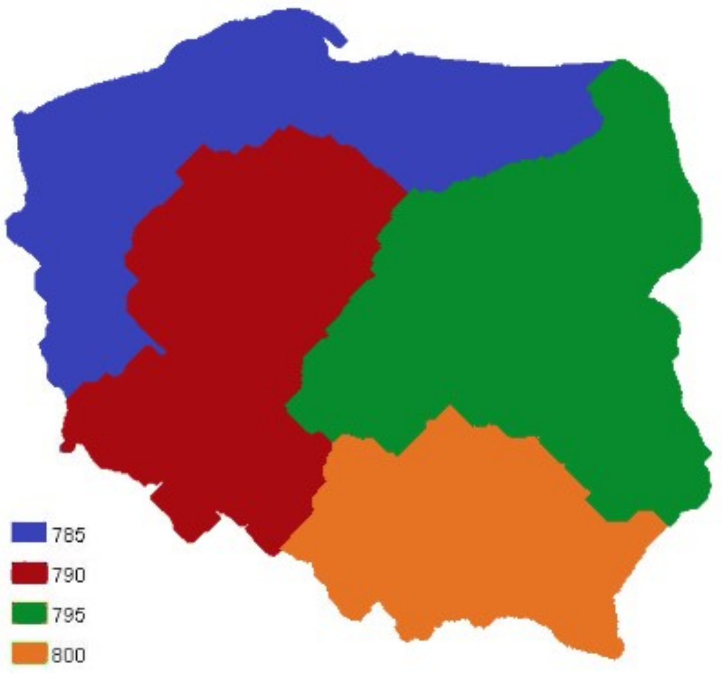The microeconomic nature of collected data also allows for the conducting of analyses in dynamic terms [77]. Formal guidelines concerning work with extremely sensitive data are subject to rigorous restrictions; thus, only the results aggregated for a minimum of 15 farms were presented in this paper. The research involved Polish regions isolated in the FADN methodology: Masuria and Pomerania, Greater Poland and Silesia, Masovia and Podlachia, as well as Lesser Poland and the Foothills (Figure 1). The study covered the period 2004–2015, where the initial year indicates the first extension of the EU to CEE countries, and the final year refers to the most recent data derived from FADN.

Out of all farms, only those characterised by continuous participation in the FADN database during the entire period under review (2004–2015) were approved for the study. The number of farms examined in individual regions is shown in

Table 1. The number of farms examined in individual regions.

Region	Pomorze i Mazury	Wielkopolska i Śląsk	Mazowsze i Podlasie	Małopolska i Pogórze
FADN designation	785	790	795	800
Number of farms	513	1566	1435	450

Source: own elaboration based on the European Union EU-FADN–DG AGRI.

.

Another novelty distinguishing the presented research results is the authors’ method of farm classification, which assumes that the increase in farm assets through investment is substantiated when it leads to a proportional increase in labour productivity. Therefore, overinvestment occurred when:

• An increase in the value of assets leads to a decrease in labour productivity, which may result from, among other things, high costs of maintaining individual assets (e.g., depreciation, insurance, repairs). Such a phenomenon was defined as absolute overinvestment.
• Increase in labour productivity is disproportionately lower than the increase in the asset value. Such a phenomenon was defined as relative overinvestment.

In the first step, changes in labour productivity were calculated for each farm. Labour productivity was defined as the amount of net value-added (gross value-added excluding depreciation), reduced by the value of subsidies for operational and investment activity per full-time employee. The use of net added value (and not the family farm income) was dictated by the need to eliminate external factors from the cost accounting (fees for hired labour, ground rent and interest on loans) to standardise economic outcomes in farms operating based on their own and external production factors. The removal of subsidies from the cost accounting results from the fact that public support should not be considered as an indicator of the economically understood labour productivity. Such an assumption may be adopted even if it is necessary (at least formally) to perform certain activities, such as meeting the cross-compliance or greening requirements, in order to obtain a particular subsidy. However, these activities involve the production of public goods, and thus they do not directly affect the economic outcomes obtained in the market. To determine changes in labour productivity, mean values were calculated for the first three and the last three years of the period under review (to eliminate incidental deviations that may occur in farms between the successive years as a result of factors beyond the producer’s control, primarily including the weather conditions). On this basis, the index of change was calculated according to the following formulae:

$$\mathsf{\Delta }LP=\left(\frac{L{P}_{2013-2015}-L{P}_{2004-2006}}{L{P}_{2004-2006}}\right)\times 100\%$$

(1)

$$L{P}_t=\frac{{\sum }_t^{t+2}(\frac{SE410-SE360-SE406-SE605}{SE010})}{3}$$

(2)

where LP: labour productivity, SE410: gross farm income, SE360: depreciation, SE406: subsidies on investments, SE605: total subsidies (excluding subsidies on investments) and SE010: total labour input (AWU).

Then, changes in the capital-labour ratio were calculated. The value of tangible assets reduced by the value of land per full-time employee was used as an indicator of an increase in the capital-labour ratio. Such an approach is justified by the fact that the problem of overinvestment ultimately concerns the maladjustment of the machinery and construction investment scale to the acreage. Similar to labour productivity, the mean values of the capital-labour ratio were calculated for the first three and last three years of the period under review. Then, the index of change was determined:

$$AL{R}_t=\frac{{{\displaystyle \sum }}_t^{t+2}(\frac{SE441-SE446}{SE010})}{3}$$

(3)

$$\Delta ALR=\left(\frac{AL{R}_{2013-2015}-AL{R}_{2004-2006}}{AL{R}_{2004-2006}}\right)\times 100\%$$

(4)

where ALR: assets-to-labour ratio (capital-labour ratio), SE441: total tangible assets, SE446: land, permanent crops and quotas and SE010: total labour input.

In the next step, each farm was assigned to a specific group based on the level of overinvestment:

Farms exhibiting absolute overinvestment, in which labour productivity declined while the capital-labour ratio increased:

$$\Delta LP<0\wedge \Delta ALR>0$$

(5)

Farms exhibiting relative overinvestment, in which both labour productivity and the capital-labour ratio increased, but the rise in the capital-labour ratio was lower than the rise in labour productivity:

$$\Delta LP>0\wedge \Delta ALR>0\wedge \Delta LP<\Delta ALR$$

(6)

Underinvested farms, in which both labour productivity and the capital-labour ratio decreased.

$$\Delta LP<0\wedge \Delta ALR<0$$

(7)

Optimally investing farms, in which labour productivity and the capital-labour ratio increased, but labour productivity rose at a faster rate than the labour-capital ratio.

$$\Delta LP>0\wedge \Delta ALR>0\wedge \Delta LP>\Delta ALR$$

(8)

In the next step, the estimation of a model that aimed to determine the technical efficiency of farms was conducted. Manufacturing efficiency analysis was determined using the stochastic frontier analysis (SFA) method. SFA allows for characterising the relations within a given industry by comparing the level of input and output of units and taking into account the occurrence of two data components: a random factor and inefficiency [79]. SFA is classified as a holistic method and is therefore used to evaluate the overall performance of an enterprise by determining various relationships between input and output. It is also a frontier method, that is, it is based on the assumption that all units should be able to operate at a certain level of efficiency. This level, often referred to as a boundary level, is determined by the model based on the efficiently operating units of a given sector. Such units are a reference for others, indicating the target range (boundary) of efficiency improvement. Model units create an exemplary level of efficiency; that is, they achieve the best results with the least input or incur the lowest costs with a specific input. SFA is a parametric method. This indicates that the functional form of the boundary value is used to estimate the costs or production function. Such methods require a more accurate knowledge of production and costs incurred. SFA estimates the efficient cost or production, taking into account the stochastic character of the input data [80].

The following analysis focuses on the technical efficiency of farms, which reflects the distance of each farm’s efficiency index from the production boundary. This measure may be estimated either in a non-parametrical way, using data envelopment analysis (DEA) [70,81], or parametrically, using SFA [80,82]. The main reason why it was decided to use SFA instead of DEA is that it separates the measurement error from the component responsible for inefficiency. Unlike other parametric benchmarking methods, SFA takes into account random disturbances that may affect the outcome of the final efficiency measurement. This fact may certainly be considered a major advantage of SFA. Taking into account the specificity of agricultural production, including dependence on weather conditions, the choice of a method that separates ineffectiveness from random variability is the only reasonable approach, especially when the research focuses on regional differences in effectiveness. Dependence on weather conditions varies regionally, especially in terms of the diverse growing season. Thanks to the landmark publications by Meeusen and van den Broeck [82] and Aigner et al. [80], parametric stochastic frontier (SF) models based on cross-sectional or panel data have become extremely valuable tools for performance analysis. These models are based on the theoretical assumption that there is an ideal “boundary” of efficiency that no economic unit can exceed, and that deviations from this boundary represent individual inefficiency. The literature distinguishes between the models of production and cost boundaries. The first approach determines the maximum amount of production that may be obtained using a particular level of input, whereas the second characterises the minimum input required to generate a given level of production. From a statistical perspective, implementation of this idea was made possible thanks to the identification of a regression model characterised by a complex error component, which includes the classical idiosyncratic disturbance resulting from the measurement error, as well as a disturbance responsible for individual inefficiency.

Originally, these models were primarily applied to cross-sectional data. Pitt and Lee [83] were the first to propose an extension of these models with time variables by estimating the following model using the maximum likelihood (ML) method:

$$\begin{array}{ccc}{y}_{it}=\alpha +{x^{\prime }}_{it}\beta +{\epsilon }_{it}& i=1,\dots ,N,& t=1,\dots ,T_i\end{array}$$

(9)

$${\epsilon }_{it}=v_{it}-u_{it}$$

(10)

$$v_{it}\sim \mathsf{{\rm N}}(0,{\sigma }_v^2)$$

(11)

$$u_{it}\sim \mathsf{{\rm N}}(0,{\sigma }_u^2)$$

(12)

A generalisation of this model, which resulted in the acquisition of the truncated normal distribution, was proposed by Battese and Coelli [84]. As Schmidt and Sickles have [85] indicated, it is also possible to perform the Stochastic Frontier model estimation using time-invariant inefficiency by adjusting conventional, fixed effect estimation techniques, thus enabling the correlation of inefficiency with the boundary regressors and avoiding assumptions concerning the ui coefficient distribution. However, time-invariant inefficiency has been called into question, particularly with regard to empirical analyses based on multi-year data sets. To reduce this limitation, Cornwell, Schmidt and Sickles [86] approached the problem by proposing the following SF model with individual-specific slope parameters:

$$\begin{array}{ccc}{y}_{it}=\alpha +{x^{\prime }}_{it}\beta +v_{it}\pm u_{it},& i=1,\dots ,N,& t=1,\dots ,T_i\end{array}$$

(13)

$$u_{it}={\varpi }_i+{\omega }_{i1}t+{\omega }_{i2}{t}^2$$

(14)

in which model parameters are estimated by extending conventional, fixed and random effects panel data estimators. This quadratic form allows for the establishment of a unit-specific model of inefficiency and requires the estimation of a significant number of parameters.

To achieve the main objective of the study, an SF model was created using the previously described panel data. Rather than develop separate models for each region or overinvestment group, a single model was intentionally built to include all farms. The significance of this approach consists of the creation of a single model of production efficiency for the entire country. Use of multiple models would make it difficult to identify differences in the scope of technical efficiency between regions or overinvestment groups. This could prove that farms from a group or region that is actually less efficient would exhibit relatively greater efficiency, as they would, on average, deviate less from the regional or group model.

In the estimated model, total output (SE131 in the FADN database) was established as the output variable, whereas the input variables included labour input (SE010), utilised agricultural area (SE025), tangible assets (total tangible assets reduced by the land value; SE441–SE446) and intermediate consumption (SE275). Cillero et al. [87] used similar variables in their research. Model estimation was performed by means of STATA 15 software (StataCorp LLC, College Station, TX, USA) using the sfpanel command.

Using the model’s estimation, it was possible to determine which part of the total variation was due to inefficiency and which was due to a random factor. During the next stage, having eliminated random errors from this rate, there was the estimation of technical efficiency for each farm in each year. The rate ranges from 0 to 1. If a farm has zero efficiency, the rate is 0. If it is a model farm and uses its input resources as efficiently as possible, the rate is 1.

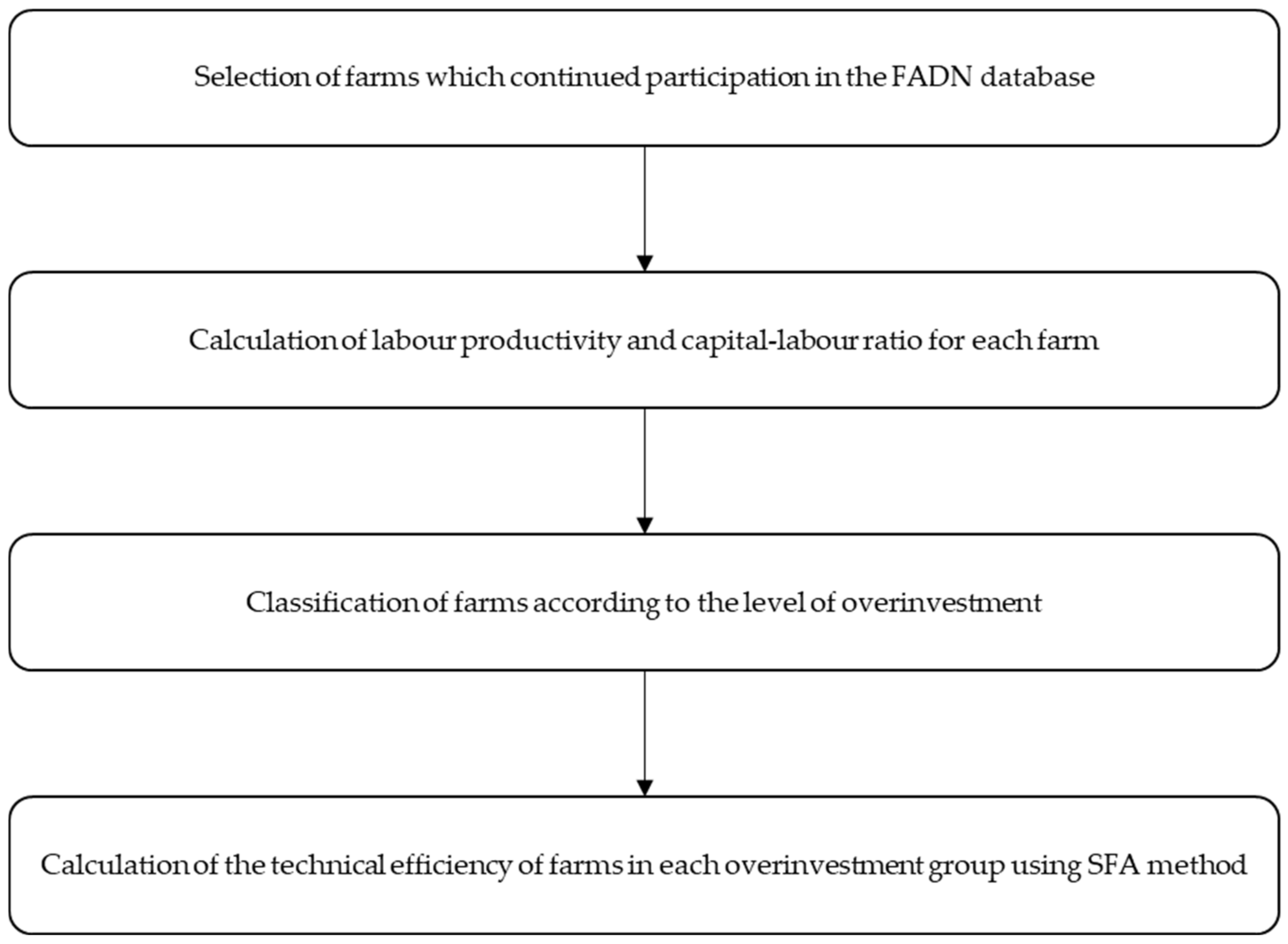
Having calculated the rates of technical efficiency based on the built model, average efficiencies were determined for individual overinvestment groups in Polish regions for 2004–2015. The averages were also calculated for marginal years, which enabled the estimation of changes in the technical efficiency of individual farms. To indicate even more precisely the changes taking place, rate histograms were also created for marginal years, which enabled not only the comparison of averages but also the analysis of changes in their distributions. In summary, regional diversity of technical efficiency in agriculture as a results of an overinvestment was measured as shown in Figure 2.

3. Results and Discussion

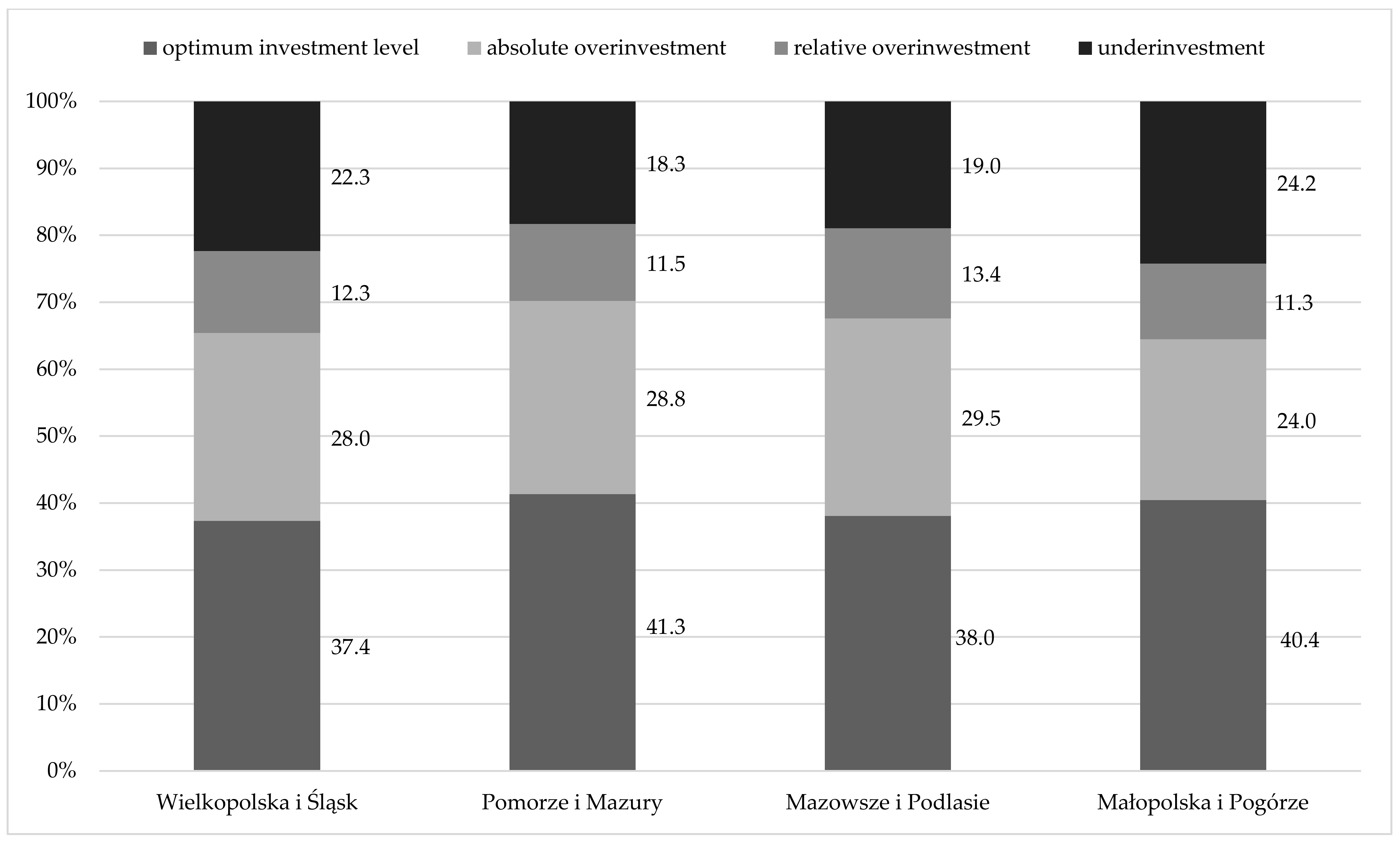
The first step for accomplishing the research objective was to classify the farms according to the overinvestment scale. According to the adopted methodology, farms with a continuity of data in the FADN database in the analysed years were classified based on changes in labour productivity and their technical equipment. The structure of farms, taking into account the overinvestment groups, proves that there are no significant differences in this respect from region to region (Figure 3). A positive aspect is the fact that optimally investing farms comprise the most numerous group in each of the regions. The less positive aspect is that there are relatively few of them, ranging from 37.4% in Greater Poland and Silesia to 41.3% in Masuria and Pomerania. It is necessary to take into account that the situation of farms exhibiting relative overinvestment is also believed to be positive. Admittedly, this group is the least numerous and diversified in all regions, but by summing up its shares with the shares of optimally investing farms, it becomes noticeable that they constitute more than half of all farms in all regions except for Greater Poland and Silesia.

The second-largest group in this structure includes farms exhibiting absolute overinvestment, where, despite an increase in the technical capital-labour ratio, their productivity decreased. In three regions, the percentage share of this group ranged from 28.0% to 29.5%; the value was 24% only in Lesser Poland and Foothills. Unfortunately, this difference results from the fact that, in this region, nearly one in four farms is underinvested in, and the share of underinvested farms is the highest among all regions. When analysing Figure 3, it is necessary to note that differences between the regions in this regard are small enough that the farm structure should be considered very similar. As a result, it is difficult to explicitly identify the best region in terms of farm structure according to the overinvestment groups.

The next step of the study was to build an SF model based on the established variables, whose descriptive statistics are shown in

Table 2. Descriptive statistics of the variables included in the model.

Zmienna (Jednostka)	Region	Mean		Std. Dev.		Min.		Max.
		2004	2015	2004	2015	2004	2015	2004	2015
SE010 (AWU)	Pomorze i Mazury	2.10	2.11	1.20	1.32	0.42	0.23	13.47	12.32
	Wielkopolska i Śląsk	2.10	2.08	1.94	1.91	0.37	0.30	47.20	49.07
	Mazowsze i Podlasie	2.00	2.01	0.99	1.20	0.33	0.21	24.69	23.77
	Małopolska i Pogórze	2.10	2.23	1.47	1.92	0.56	0.44	16.60	24.45
SE025 (ha)	Pomorze i Mazury	53.04	60.42	108.06	94.32	0.00	0.00	1889.00	1325.00
	Wielkopolska i Śląsk	33.93	42.15	54.15	59.29	0.08	0.00	1402.00	1360.65
	Mazowsze i Podlasie	19.95	27.07	20.89	26.83	0.08	0.08	422.48	359.57
	Małopolska i Pogórze	19.37	27.77	24.71	40.68	0.00	0.00	230.00	499.00
SE441–SE446 (tys. EUR)	Pomorze i Mazury	77.31	130.23	82.44	181.21	4.82	2.61	812.29	1803.19
	Wielkopolska i Śląsk	80.59	122.37	72.95	154.08	1.07	0.00	843.81	3114.66
	Mazowsze i Podlasie	62.59	97.16	51.96	114.82	1.76	0.57	655.19	1035.57
	Małopolska i Pogórze	71.20	106.80	99.33	154.08	3.54	0.95	1573.82	1210.09
SE275 (tys. EUR)	Pomorze i Mazury	31.34	61.48	74.84	141.11	1.44	1.62	1013.58	1877.36
	Wielkopolska i Śląsk	28.87	48.91	37.52	71.62	1.01	1.92	872.49	966.10
	Mazowsze i Podlasie	13.74	29.01	22.01	45.67	0.60	1.52	392.14	922.19
	Małopolska i Pogórze	18.08	33.30	34.41	56.54	1.35	1.60	432.19	684.00
SE131 (tys. EUR)	Pomorze i Mazury	50.74	92.65	106.00	215.97	3.37	2.36	1415.692	3048.95
	Wielkopolska i Śląsk	43.82	73.43	56.18	107.85	2.07	0.87	1205.53	1690.85
	Mazowsze i Podlasie	25.22	46.52	33.14	66.47	0.00	1.21	456.63	922.19
	Małopolska i Pogórze	31.72	57.92	47.48	100.52	3.31	2.05	554.04	1427.74

Source: own elaboration based on EU-FADN–DG AGRI; STATA 15.

. On this basis, it is also possible to draw some conclusions concerning the differentiation of individual regions and the dynamics of changes. Certainly, the statistics relate only to the farms included in the FADN database and, additionally, only those maintaining continuity in the said database; hence, the values of the variables differ from those provided by Eurostat. In addition, differences may result from the fact that the FADN database includes only commercial farms and, in overall statistics, subsistence farms.

In the case of labour resources (SE010), all regions have a similar average number of full-time employed persons, oscillating around 2, while the greatest variation measured by standard deviation is found in Greater Poland and Silesia. This means that the amplitude of the variable’s values is greatest in this region.

The situation is different for the average utilised agricultural area (SE025) of the farms included in the FADN sample. Such differences are significant, and in some cases, are even double. The largest farms are located in Masuria and Pomerania, and the smallest ones are in Masovia, Podlachia, Lesser Poland and the Foothills, which may affect the results concerning overinvestment and efficiency. In dynamic terms, the agricultural area increased over the analysed years in all regions. In relative terms, the greatest increase was observed in the regions with the lowest initial agricultural area. It should also be noted that there was a decrease in variation in Masuria and Pomerania, and an increase in variation in Lesser Poland and the Foothills. Furthermore, in three out of the four regions, the initial areas of the largest farms decreased, which may also indicate a reduction in polarisation.

The differences between regions were also visible in terms of providing farms with tangible assets (a value of SE441 variable minus a value of SE446 variable). However, in this case, the variation was not as large as the one concerning their area. In all regions, farms increased the value of tangible assets owned. The standard deviation, however, also significantly increased, which in turn may indicate increasing polarisation in this regard. An increase in the value of tangible assets owned by farms with simultaneous stabilisation in labour resources indicates that there is a global increase in technical work equipment, which is one of the indicators that determine belonging to a particular group in accordance with the adopted classification of farms. It should also be noted that only farms classified as underinvested, accounting for approximately 20% of all farms, decreased their level of technical work equipment.

Both the increase in the average agricultural area and tangible assets provision were accompanied by an increase in intermediate consumption. These Figures were established as the basic measure of the costs of working capital consumption, for which the regions differed significantly. It can be concluded that in so far as farms expand and invest in tangible assets, they also want to intensify production, which implies an increase in the consumption of means of production that largely include intermediate consumption. Indeed, the SE275 variable is the sum of direct costs of plant production (seeds, seedlings, fertilisers, plant protection products), animal production (fodder) and economic overheads (related to operating activities but not recognised as direct operating costs).

The output variable in the estimated model was total output (SE131), which is the sum of the value of plant production, animal production, and other production, primarily intended for sale or consumed in internal production, and transferred, to a small extent, to the household. In this respect, there is considerable variation across the studied regions; however, as with other categories, the average total output increased in each region. The amplitude and variation measured by standard deviation simultaneously increased as well, which may also be indicative of increasing farm polarisation.

The estimation results of the stochastic model are shown in

Table 3. Parameters of the estimated SFA model.

SE131	Coef.	Std. Err.	z	P > |z|	[95% Conf. Interval]
Frontier
SE010	4026.773	371.3045	10.84	0.000	3299.03	4754.516
SE025	254.2794	20.62924	12.33	0.000	213.8469	294.712
SE275	0.8972276	0.010069	89.11	0.000	0.8774928	0.9169624
SE441–SE446	0.1150276	0.0050351	22.85	0.000	0.105159	0.1248962
Usigma
_cons	18.66797	0.0313604	595.27	0.000	18.6065	18.72943
Vsigma
_cons	21.05943	0.0164298	1281.78	0.000	21.02723	21.09163
sigma_u	11,316.12	177.4392	63.77	0.000	10,973.64	11,669.29
sigma_v	37,410.77	307.3256	121.73	0.000	36,813.24	38,017.99
lambda	0.302483	307.798	0.00	0.999	−602.9705	603.5754

Source: own elaboration based on EU-FADN–DG AGRI; STATA 15.

. Wald Chi-Squared statistics were used for testing the null hypothesis, according to which all regression coefficients are simultaneously equal to zero in both models. The small p-value obtained from the test, <0.0001, leads us to accept the alternative hypothesis, according to which at least one of the regression coefficients in the model is not equal to zero. The p-values of the statistics for each variable confirm that each of them is statistically significant, even at a significance level of 0.001.

The coefficients determine the course of the SF for each variable. It can be assumed with a 95% confidence level that an increase in the number of employees by one unit will result in an increase in the output of between 3299.03 and 4754.52. An increase in the agricultural area by one hectare will result in an increase in the output of between 213.85 and 294.71 euros, whereas an increase in fixed capital by one euro will result in an increase in the output of between 0.105 and 0.125 euros. A puzzling aspect is a coefficient value for the intermediate consumption variable, whose 95% confidence interval ranged from 0.87 to 0.92. This means that if intermediate consumption increases by one euro, the output will increase by less than one euro. There may be several reasons for this situation. First of all, it seems possible that farms increasing the output intensity even further enter the zone of decreasing economies of scale, in which an increase in the output does not fully compensate for the additional incurred costs. This could be the case for the use of either inefficient, high-level fertilisation or overly intensive pest management programs, or for where non-optimal animal nutrition is provided. This situation shows that production optimisation, primarily by using cost accounting, is more important from the point of view of economic efficiency than production increase. From a practical point of view, it can also provide guidance for an even more careful use of the economic damage thresholds, which are recommended by integrated pest management, and for more balanced nutrition in terms of animal production.

A correlation of intermediate consumption with inefficiency might be another attempt to explain this situation. According to formula 9, the total model variation consists of two components, i.e., inefficiency and random disturbances. After the total variance was calculated, it turns out that inefficiency accounts for 8.38% of variation, whereas random disturbances cause 91.62% of existing variation. Certainly, random variation in agriculture can result from a number of factors, from weather through changes in agricultural markets to political instability. While the labour, land and fixed capital resources are relatively fixed and difficult to change in a short period of time, the direct costs of production, constituting intermediate consumption, may be the most susceptible to the above-mentioned random disturbances. On the other hand, a farmer can be most responsive to random disturbances through direct cost management.

The high, over 90%, proportion of random variation to total variation should also indicate another extremely important issue related to insurance in agriculture. The fact that most farms are exposed to various types of risks that can affect production efficiency makes it extremely important for the stable functioning of farms to transfer the risk to an insurance entity. Then, in the case of damage caused by various factors, the farmer may lose part of the output. However, they will not lose income, which will enable them to continue functioning in a stable manner.

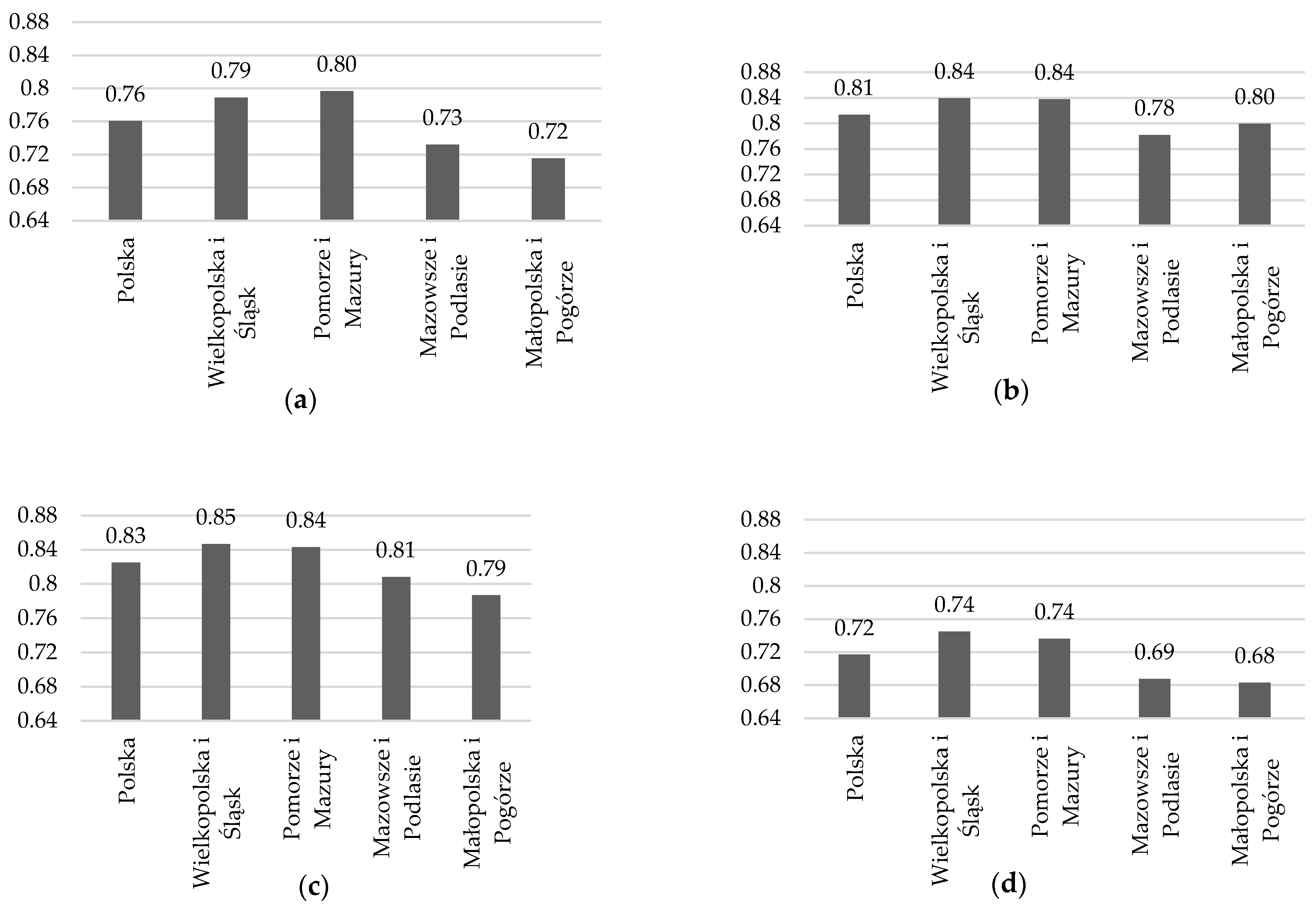
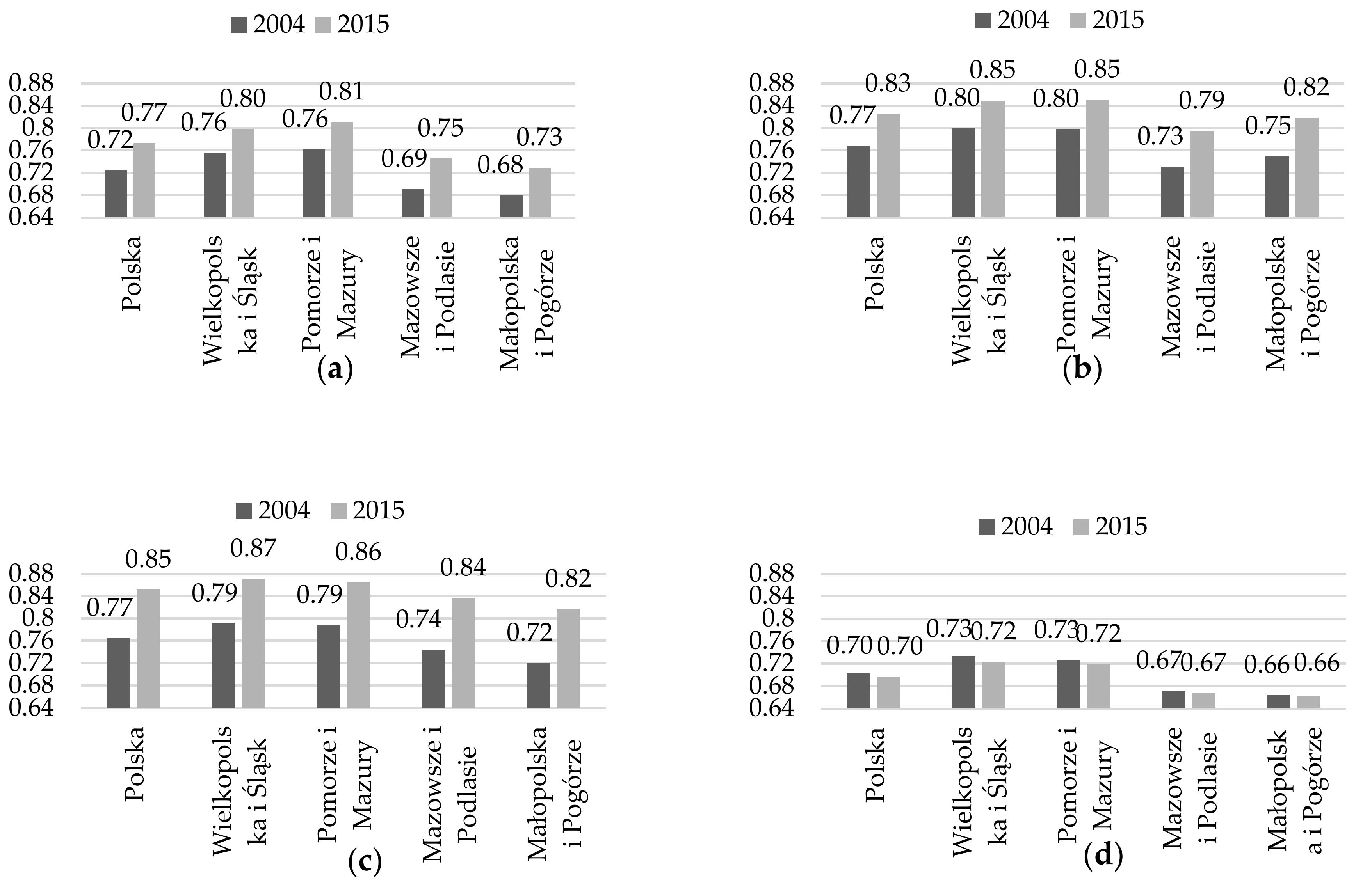
A key part of the study involved determining the technical efficiency of each farm based on the built SF model. The average values of the technical efficiency index were then calculated separately for each region and overinvestment group. This enabled identification of regional differences in terms of the established measure.

Figure 4 shows the average technical efficiency of farms in individual regions of Poland depending on the overinvestment group during the period 2004–2015. There are noticeable differences in the average technical efficiency for different overinvestment groups, ranging, for the country as a whole, from 0.72 for underinvested farms to 0.83 for relatively overinvested farms. Given the nature of the agricultural sector, this inconspicuous difference in manufacturing efficiency can strongly translate into farm viability and profitability. It should be taken into account that the viability level in agriculture is frequently only a few percent. Thus, if a farm is 11% less efficient, that is very likely the reason it may be incurring losses in operations.

Interestingly, optimally investing farms do not have the highest technical efficiency. The farms with the highest technical efficiency include relatively overinvested farms in Greater Poland, Silesia, Masovia and Podlachia and absolutely overinvested farms in Lesser Poland and the Foothills. In the case of Masuria and Pomerania, the same, on average, efficiency was achieved by both relatively and absolutely overinvested farms. Underinvested farms are the least efficient in all regions. This is due to the fact that in order to produce efficiently, it is necessary to at least maintain the level of tangible assets provision, and preferably to increase it as well.

Differences are also revealed on a regional basis. In all groups, the most efficient farms are located in Greater Poland and Silesia, as well as in Masuria and Pomerania, where the average efficiency in each group is higher by several percent than in Masovia and Podlachia or in Lesser Poland and the Foothills. Those differences are significant enough to state that the group of underinvesting farms in two more efficient regions has higher average technical efficiency than farms that optimally invest in the other two regions.

The results given in Figure 4 are the average results for 2004–2015; hence, they do not take into account the changes that may have occurred in farms over the analysed period. Therefore, the average technical efficiency for the marginal years in each group was calculated so that the dynamics could be identified in each group and region (Figure 5).

The key and primary finding of the study is that average technical efficiency, only for the group of underinvested farms, did not increase in any of the regions, mostly remaining at a similar or slightly lower level. In other groups, regardless of the region, the efficiency increased by at least several percentage points (from 0.04 in Greater Poland and Silesia in the group of optimal farms up to 0.10 in Masovia and Podlachia, as well as in Lesser Poland and the Foothills, in the group of relatively overinvested farms).

It should also be noted that, as a rule, the greatest change dynamics took place in regions where the initial efficiency was the lowest. On the one hand, this may indicate the use of development opportunities of regions with the weakest agricultural structure (as highlighted by discussing descriptive statistics of variables adopted in the model). On the other hand, it may indicate decreasing marginal effectiveness. The more efficient a farm is, the more difficult it becomes to increase that efficiency. This is demonstrated by practical terms of production: for example, each additional fertiliser unit has a decreasing proportion in production. Moreover, beyond a certain limit, an increase in the use of fertilisers may even cause a decrease in production.

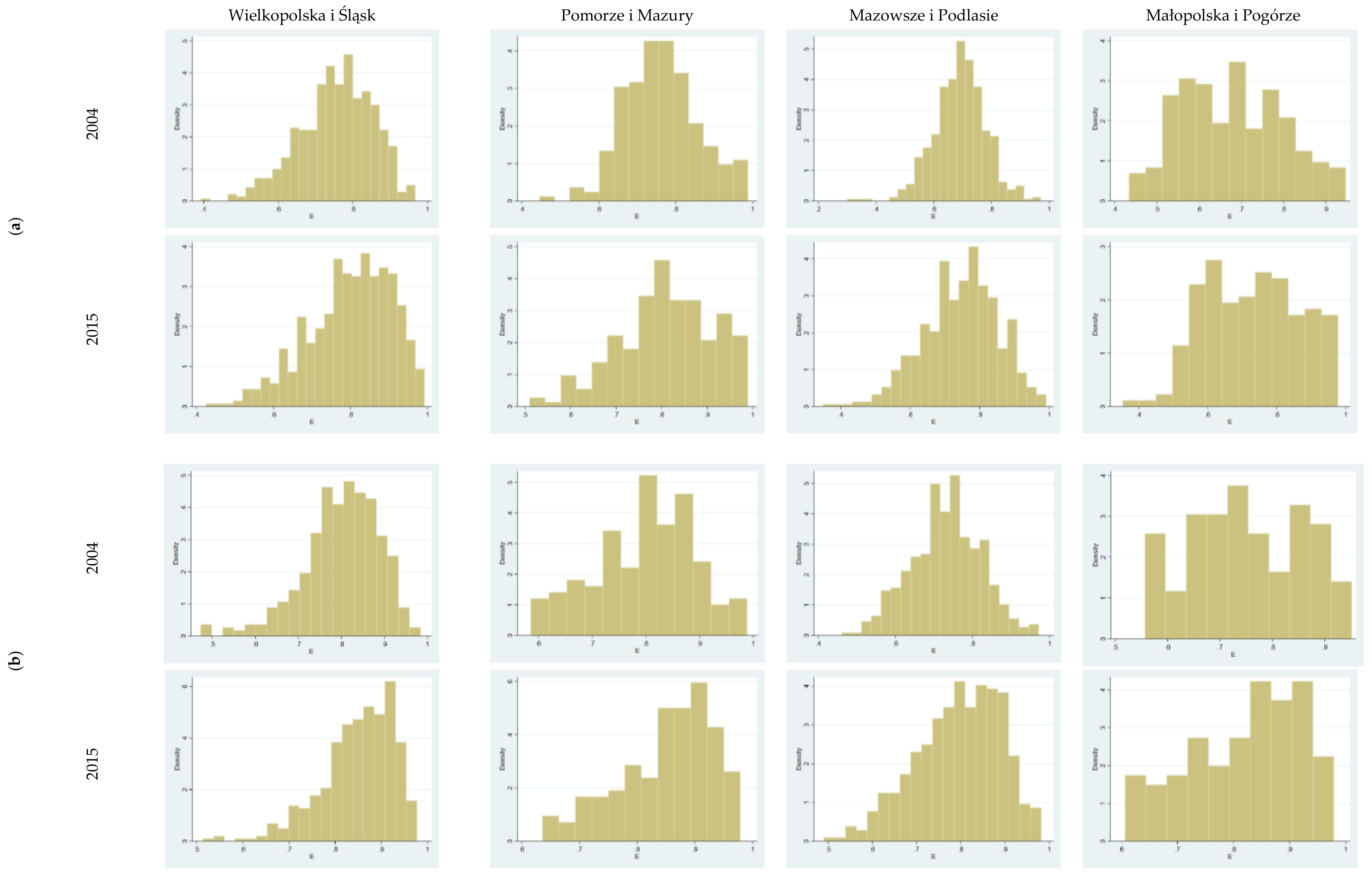
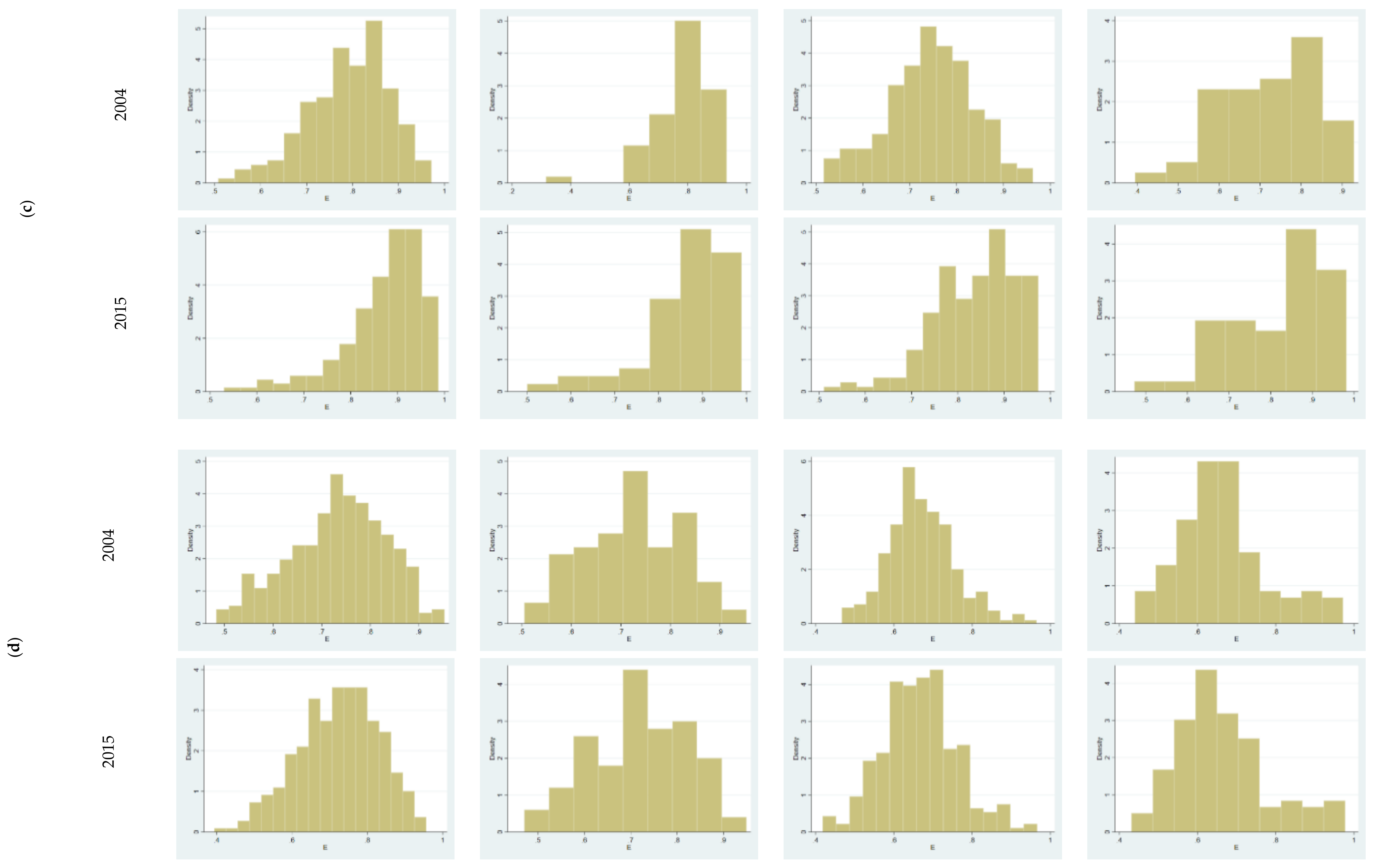
The presented histograms of the technical efficiency distribution of farms (Figure 6) confirm the relationships described above. For the first three groups, there was a clear distribution shift to the right, indicating a general improvement in the structure of farms according to their efficiency. The distribution in question did not improve, and in some regions even worsened, only for the group of underinvested farms.

4. Conclusions

From the theoretical and methodological point of view the methodical approach used in this study, which consisted of conducting an original classification of farms according to their level of overinvestment and a further measurement of technical efficiency using the SF approach, turned out to be a useful tool for determining regional differences that occurred as a result of overinvestment. It enabled the indication of important relationships that were presented in the literature review, but which had never before been noted at the micro level of FADN farms in regional comparison.

The results indicate a significant problem of investment scale in relation to farm efficiency. About 40% of farms in Poland the scale of investments can be assessed as optimal, more than quarter of farms exhibited absolute overinvestment and nearly one in five farms is underinvested. However, on a regional basis, the structure of farms in terms of the level of overinvestment does not significantly differ across regions of Poland. Nevertheless, there are differences between regions in terms of farm efficiency within each group. In all regions, only the underinvested farms did not increase their efficiency over the period under review. The highest efficiency growth rate occurred in regions where farms were least efficient at baseline. These results indicate a significant problem of inability to improve farm efficiency. The investments that show a correlation to the level of efficiency achieved provide a clue. Indeed, although underinvestment in this area affects the lack of efficiency growth.

This yielded important results provide a guidance for more careful investment planning by farmers. When planning investments farmers should take into account their effect in the form of changes in the effectiveness of the production factors used. The results may also have implications for agricultural policy. Programming the regional allocation of pro-investment funds should take into account regional differences of the agricultural sector in terms of providing farms with tangible assets and efficiency of production. The allocation of funds should take into account the leveling of regional disproportions while minimizing the potential incentives to overinvestment.

All studies indicate the significance of the raised problem This highlights the need for a future focus on the raised problem of overinvestment, as well as the identification of possible causes of the studied phenomenon. It seems advisable to make some modifications for further research, which could provide an even more solid foundation for inference. It may be appropriate to divide farms according to agricultural type, as differences may be due to the regional specificity of agricultural production. In this way, each direction of production has different conditions that determine efficiency. Along the same lines, it may be useful to build a separate model for each region or agricultural type. This will enable determination of the SF for each type of activity to locate the greatest inefficiency and determine where random disturbances are primarily responsible for the variation.