Effectiveness of Artificial Neural Networks in Hedging against WTI Crude Oil Price Risk

Abstract

Despite the growing share of renewable energy sources, most of the world energy supply is still based on hydrocarbons and the vast majority of world transport is fuelled by oil products. Thus, the profitability of many companies may depend on the effective management of oil price risk. In this article, we analysed the effectiveness of artificial neural networks in hedging against the risk of WTI crude oil prices increase. This was reformulated from a regressive problem to a classification problem. The effectiveness of our approach, using artificial neural networks to classify observations, was verified for over ten years of WTI futures quotes, starting from 2009. The data analysis presented in this paper confirmed that the buyer of a call option was more often likely to incur a loss as a result of its purchase than make a profit after the final payoff from the call option. The results of the conducted research confirm that neural networks can be an effective form of protection against the risk of price fluctuations. The effectiveness of a network’s operation depends on the choice of assessment indicators, but analyses show that the networks which, for the indicator that was selected, gave the best results for the training set, also resulted in positive rates of return for the test set. Significantly, we also showed interdependence between seemingly unrelated indicators: percentage of the best possible results achieved in the analysed period of time by the proposed method and percentage of all available call options that were purchased based on the results from the networks that were used.

1. Introduction

In today’s world, crude oil is one of the most important resources. It is a leading fuel and its price has a direct effect on the global economy, oil exploration and exploitation, as well as many other activities. Crude oil plays a key role in numerous areas of the world economy as an input in the production of numerous types of goods in many sectors of the economy. Crucially, despite the quickly growing share of renewable energy sources, transport and delivery of almost all goods and many services still rely on crude oil.

Previous studies have shown that crude oil price fluctuations have a significant impact on the level of economic activity and consumer sentiment. This correlation was especially noticeable during the financial crisis in 2007–2008 [1]. There has also been a lot of research on the relation between oil prices and the rate of real GDP growth, unemployment, and inflation rate in the USA [2,3,4,5,6,7,8] and other countries [9,10] as well as general studies on the impact of commodity price volatility on growth [11].

Literature has also identified the impact of oil price shocks on macroeconomic aggregates such as the level of investment, stock prices and returns [12,13,14,15,16,17], inflation rate [18], industrial production and exchange rates [19,20,21,22,23], as well as financial and monetary policy [24]. There has also been a large number of studies concerning the impact of crude oil prices on various groups of commodities such as: gold [25,26], silver, platinum and palladium [27], zinc, copper and molybdenum [28], agricultural [29,30,31,32], and energy commodities [33,34,35,36,37].

The impact of oil prices on the level of countries’ risks is also an increasingly popular subject of research. Liu et al. [38] have suggested that properties of country risk remain comparatively steady despite the oil price volatility. They have also found that oil price fluctuations can expand a country’s risk under some special conditions. Said-Zada identified technical progress as an important additional source of economic modernisation [39]. In turn, Lee et al. [40] investigated the dynamic relationship between oil price shocks and country risk using a Structural VAR framework for a sample of both net oil-exporting and net oil-importing countries. They have shown that positive oil price shocks trigger a reduction in country risk for net oil-exporting country. The opposite is also true. The issue of risk and oil prices was also discussed by Lee and Yoon [41]. They found the effect of volatility spillover from the Brent oil market to the European Union carbon emission allowance (EUA) market. They also showed that investors can effectively hedge their investment risk by holding EUAs and energy sources together as assets. Zeng and others investigated the dynamic volatility spillover effect between EUAs and similar market-based approaches [42].

Numerous studies showing the impact of fluctuations in crude oil prices on macroeconomic indicators and the level of risk incurred by countries and enterprises in various industries, confirm the importance of effective hedging against resource price changes. However, to the best of our knowledge existing papers have focused on price forecasting and regression, whereas we have reformulated this to a classification problem, which can be a useful approach, especially on the commodity derivatives market.

Derivatives are one of the instruments that can support the price risk management process. Moreover, due to the variety of delivery methods for raw materials and other products (their completion is assigned to a specific moment in the future), they constitute an important part of commodity exchanges. Nonetheless, the misuse of derivatives may be perceived as an additional source of risk, based on the events preceding the 2007–2008 financial crisis.

For long options, that are the subject of our research, the maximum loss is limited and equal to the value of the total option premium (the unit option premium multiplied by the number of options that were bought). This makes it possible to use long options as a tool offering protection against unfavourable changes in oil prices, without generating additional risk. Furthermore, taking a long position in a call option does not require the buyer to make an initial deposit or add to it during the term of the contract. Therefore, the only cost for the option buyer is the option premium, which is paid on the day the position is opened. It is also worth noting that this amount is known and it is up to the buyer to decide whether or not to accept this cost.

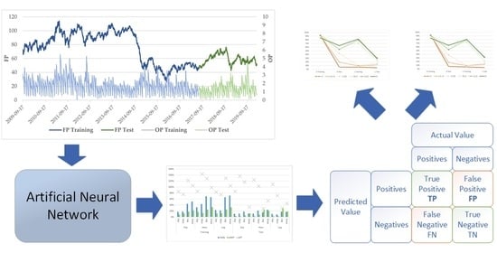
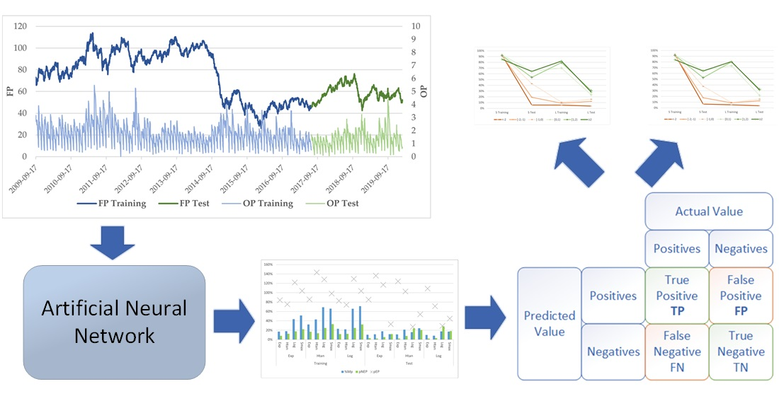
The main aim of this paper is to analyse the effectiveness of using artificial neural networks in search for buy signals for European call options, referring to the nearest expiration date for future contracts on WTI crude oil (front month futures).

The choice of artificial neural networks (ANNs) to search for option buy signals was dictated by the complexity of this problem. ANNs are nonlinear methods that imitate the human brain. They are characterised by: self-organisation, data-driven memory, self-learning, self-adaptation and associated memory [43]. ANNs use large amounts of processed information and can capture hidden functional relationships in data, even if the functional relationships are unknown or difficult to identify.

In order to choose ANNs as a tool to support the decision-making process in the crude oil options market, we were also influenced by numerous attempts to use this tool in oil price prediction. Azadeh et al. [44] used a flexible algorithm based on ANNs and fuzzy regression (FR) to forecast annual oil prices. They showed that the selected ANNs models considerably outperform the FR models in terms of mean absolute percentage error (MAPE). Chiroma et al. [45] proposed an approach based on a genetic algorithm and neural network (GA–NN) for the prediction of WTI crude oil prices. Mann–Whitney test results indicated no significant difference between median WTI crude oil prices predicted by GA–NN and prices observed from May 2008 to December 2011. In turn, Wang and Wang [43], in an attempt to forecast crude oil prices and oil stock prices, used a combination of multilayer perception (MLP), and Elman recurrent neural networks (ERNN) with stochastic time effective function (ST) to develop a forecasting model, called ST-ERNN. The forecasting results of the proposed model were more accurate than the backpropagation neural network (BPNN) and ERNN models. The issue of volatility forecast and option-trading strategy was explored by Liu and others using an improved Artificial Bee Colony with Back Propagation (BP) natural network model. They found that the ANN model is better at predicting implied volatility than for example Monte Carlo simulation [46].

These and other ANNs models [47,48,49,50,51,52,53,54,55,56] have shown that ANNs provide an important alternative to econometrics (both linear and nonlinear) in forecasting crude oil prices. Dbouk et al. [57] noted, however, that the accuracy of price predictions is not a key aspect of successful investment or hedging strategies. It is also worth noting that the main aim of our research was not to use the ANNs to predict future oil prices, but to search for call options purchase signals with the use of this tool. There are currently no studies other than our previous article [58] that consider hedging against changes in prices of oil (and other raw materials) as a classification problem. In the case of options market participants, especially buyers, the problem of the correct classification (profit or loss) of the return on hedging is particularly important. Based on copious market data, buyers must make quicks decision whether the purchase of options at a given point in time will be an effective form of hedging against oil price fluctuations in the future. In our opinion, using ANNs to make this type of decisions may facilitate hedging against oil price changes. Thus, this paper focused on finding network parameters that maximise network effectiveness indicators which are defined later in the study.

This paper builds on an approach proposed by the authors in [58]. In order to be able to extend the results, the analyses are carried out on the same data set. To the best of our knowledge, that was the only study until now indicating that neural networks can be a useful tool supporting the process of managing the risk of changes in oil prices using option contracts. Significantly, in this study, we showed the interdependence between two seemingly unrelated network indicators—the first assessing the quality of the network and the second the share of options that were purchased.

The dataset that was used covers the period of time from 16 June 2009 to 14 February 2020. In this paper, we present an analysis based on new network effectiveness indicators which are directly related to the hedging costs (sum of option premiums) and the number of buy signals generated by a given network. These indicators had a significant impact on the analysis and our final results.

The remainder of this article is structured as follows: Section 2 presents the proposed method: the commodity option pricing (Section 2.1), multilayer perception structure (Section 2.2) and network quality assessment indicators that we use (Section 2.3). Section 3 provides data and reports its statistical properties. Our empirical results are introduced in Section 4. The summary, conclusions and future research directions are presented in Section 5.

2. Proposed Methods

We propose a tool to support decision-making processes on the crude oil option market. To hedge against the risk of oil price increases, we took long positions in call options. This approach can also be used for other commodities. The proposed tool uses multilayer perceptron neural networks. In turn, the indicators presented in Section 2.3 were chosen to evaluate the effectiveness of neural networks to search for call options buy signals.

2.1. WTI Crude Oil Options and their Parameters

The research focuses on WTI crude oil options available in the New York Mercantile Exchange (NYMEX). This is a commodity futures exchange owned and operated by CME Group of Chicago. The underlying asset in crude oil options on NYMEX is a WTI Light Sweet Crude Oil future contract (symbol: CL). Crude oil futures are settled based on the price of the WTI oil delivered to Cushing, Oklahoma. Each CL contract is equal to 1000 barrels. The contracts trade in increments of one cent per barrel [59].

A light sweet crude oil option on the NYMEX expires three business days prior to the underlying futures contract (CL). The analysed option contract is a European Style option cash settled on the expiration day. The expiration cycle of the crude oil option contract is monthly. On expiration of a call option, the option payout will be the settlement price of the CL contract minus the strike price multiplied by 1000 barrels, or zero, whichever is greater [60]. In our empirical section, we analyse the options underlying the price of the first (nearest) crude oil futures contract. Hence, the number of days until the expiry of the option ranged from 34 to 1. For the option pricing model, we used the equation proposed by Fisher Black in 1976 [61]. The Black model is a variant of the Black–Scholes option pricing model. Its basic application is for pricing options on futures contracts (mainly commodity options). The Black model is based on the assumption that prices are the random motion of particles suspended in a medium (Brownian motion—a case of stochastic Wiener process). In turn, calculation of the option premium focuses on searching for a value balancing the payout for the option buyer on the expiration day [62,63]. Eventually, with regard to the initial assumptions, prices of European commodity call options are expressed with the following equation [62,64]:

$$o{p}_c=e^{-r^{d}T}\left[f_{0}N\left(d_1\right)-KN\left(d_2\right)\right],$$

(1)

where

$$d_1=\frac{\ln \left(\frac{f_0}{K}\right)+\frac{{\sigma }^2}{2}T}{\sigma \sqrt{T}},$$

(2)

$$d_2=\frac{\ln \left(\frac{f_0}{K}\right)-\frac{{\sigma }^2}{2}T}{\sigma \sqrt{T}}$$

(3)

and

• $o{p}_c$—price of the call option (option premium),
• $f_0$—the future price of the underlying asset on the day of opening position
• $K$—strike price,
• $r^d$—risk-free interest rate (p.a.),
• $T$—time to expiry (years),
• $\sigma$—volatility of future price in the analysed period (per year),
• $N$—cumulative distribution function of the standard normal distribution

In our study, we include only ATM (at-the-money) options, i.e., those with strike price (almost) identical to the WTI future price on a given day. ATM options data were sourced from the QuikStrike platform provided by CME Group [65].

2.2. Artificial Neural Networks

In the paper, the Statistica software (TIBCO Software Inc, Palo Alto, CA, USA) was used to build artificial neural networks. The analysed networks were classification networks. In this paper, Multilayer Perceptron was used. MLP is one of the most prevalent neural networks with the ability of complex mapping between inputs and outputs, which make it possible to approximate nonlinear functions [43]. These are networks with unidirectional information flow (a class of feedforward ANNs).

The networks used in the study consist of three layers, i.e., the input layer, one hidden layer and the output layer. The Broyden–Fletcher–Goldfarb–Shanno algorithm [66] was used as a training algorithm. The number of neurons in the hidden layer of the network was set ranging from 5 to 80. In the hidden layer, five different types of activation functions were used: sine, hyperbolic tangent, exponential, linear and logistic. In addition to the above the softmax function was implemented in the output layer.

The proposed method of determining the time of hedging with the use of an ANN is referred to as SANN (due to the use of the Statistica software for creating neural networks). The result of using SANN was to obtain information on whether to buy the call option or not. The task of the network is therefore to solve the classification problem by searching for call option buy signals. The signals being sought are referred to in short as ‘buy signals’.

2.3. Network Quality Assessment Indicators

In our considerations, we assumed that no more than one option contract can be purchased on a given day. In order to be able to assess the performance of individual networks, we started off by using indicators proposed in [58]. Additionally, we calculated indicators relating to the number and value of option premiums. It should be noted that SANNs are trained in a way that maximises the number of correctly classified signals (accuracy). Hence, the given indicators should be considered as the indicators of network evaluation for which the training process has already been completed. Below we present symbol designations, the definitions and the methods of calculating each of these indicators (in four categories).

Let C be a set, whose elements are observation and C′ is a subset of the set C ($C^{\prime }\subset C$).

• Indicators referring to the maximum profit that could be achieved in the given period by taking long positions in call options.

  (a)

  MP (Maximum profit)—the sum of profits from the long call options for all days for which the final result from taking this position was greater than zero (the option was exercised with payout exceeding the value of the option premium); the value of MP index is calculated based on the following equation:

  $$MP={{\displaystyle \sum }}_{c\in C^{\prime }}{z}_c·v_c,$$

  (4)

  where c is an element of the set C′ and z_c denotes a binary variable described by the following equation:

  $$z_c=\left\{\begin{array}{l}1, if v_c>0\\ 0, if v_c<0\end{array}\right.$$

  (5)

  The variable v_c denotes the value of the final results from the purchase of the call option for observation c and it is described by the formula:

  $$v_c=max\left\{f-K;0\right\}-o{p}_c,$$

  (6)

  where

  • F—the future price of the underlying asset on the day of the option’s expiration (for options on futures);
  • K—strike price of the option;
  • op_c—option premium (for the strike price K) for observation c.

  (b)

  pMP—it is the ratio of the sum of the final results for the call options that brought profit in the given period to the sum of the option premiums paid to open these positions.

  $$pMP=\frac{{{\displaystyle \sum }}_{c\in C^{\prime }}{z}_c·v_c}{{{\displaystyle \sum }}_{c\in C^{\prime }}{z}_c·o{p}_c}$$

  (7)

  (c)

  pNMP—indicator showing the ratio of the number of days on which the options brought profit to the number of all options available in the given set of observations:

  $$pNMP=\frac{1}{\left|C^{\prime }\right|}{\displaystyle \sum }_{c\in C^{\prime }}{z}_c$$

  (8)

  where |C′| is the cardinality of a set C′. It was assumed that only one call option can be purchased on a given day, therefore the value of |C′| should be understood as the number of all call options that were available in the given period.

• Indicators referring to the maximum loss that could be achieved in the given period by taking long positions in call options.

  (a)

  ML (Maximum loss)—the sum of all losses from the long call options in a given period; the following formula is used to calculate the value of the ML indicator:

  $$ML={\displaystyle \sum }_{c\in C^{\prime }}{s}_c·v_c$$

  (9)

  where s_c denotes a binary variable described by the following formula:

  $$s_c=\left\{\begin{array}{l}1, if v_c<0\\ 0, if v_c>0\end{array}\right.$$

  (10)

  (b)

  pML—the percentage of capital loss due to the purchase of loss-making options. This indicator is assigned to a value ranging from [−1;0). The value −1 indicates a complete loss of the asset involved in options.

  $$pML=\frac{{{\displaystyle \sum }}_{c\in C^{\prime }}{s}_c·v_c}{{{\displaystyle \sum }}_{c\in C^{\prime }}{s}_c·o{p}_c}$$

  (11)

  (c)

  pNML—the share of loss-making options to the total number of considered observations:

  $$pNML=\frac{1}{\left|C^{\prime }\right|}{\displaystyle \sum }_{c\in C^{\prime }}{s}_c$$

  (12)

• Indicators referring to the result that could be achieved in the given period by taking long positions in call options.

  (a)

  AR (Average return)—the total value of the final result from the long call options on each successive day of quotation in a given period; the AR indicator is described by the following equation:

  $$AR={\displaystyle \sum }_{c\in C^{\prime }}{v}_c=MP+ML$$

  (13)

  (b)

  pAR—the percentage indicator of the amount of return on investment for all observations in the given set of observations:

  $$pAR=\frac{{{\displaystyle \sum }}_{c\in C^{\prime }}{v}_c}{{{\displaystyle \sum }}_{c\in C^{\prime }}o{p}_c}$$

  (14)

• Indicators presenting the results obtained with the use of a given neural network.

  (a)

  EP (Expected Profit)—represents the result of the neural network operation on the subset C′; the value of the indicator is obtained from the following equation:

  $$EP={\displaystyle \sum }_{c\in C^{\prime }}{o}_c·v_c$$

  (15)

  where the value o_c is described by the equation:

  $$o_c=\left\{\begin{array}{c}1, if for observation c, a call option was bought\\ 0, if for observation c, a call option was not bought\end{array}\right.$$

  (16)

  (b)

  %MP (percent of maximum profit)—the percentage of the best possible result (MP) achieved by this method (EP); the value of the %MP is obtained from the following equation:

  $$\%MP=\frac{EP}{MP}·100\%$$

  (17)

  (c)

  pEP—the quotient of the EP index and the sum of all paid option premiums from the C′ period. Its value is expressed by the equation:

  $$pEP=\frac{{{\displaystyle \sum }}_{c\in C^{\prime }}{o}_c·v_c}{{{\displaystyle \sum }}_{c\in C^{\prime }}{o}_c·o{p}_c}$$

  (18)

  The following indicator describes the profit (loss) earned with the use of a given network, considering the total cost of hedging. Since v_c is not less than –op_c, the value of the pEP index is a number not less than −1. This indicator would equal −1 if all call options purchased in the period C′ were not exercised. The maximum value of the pEP index is potentially unlimited.

  (d)

  pNEP—the indicator that shows the percentage of all available call options that were purchased on the basis of the used networks; pNEP was defined with the following equation:

  $$pNEP=\frac{1}{\left|C^{\prime }\right|}{\displaystyle \sum }_{c\in C^{\prime }}{o}_c$$

  (19)

Indicators from categories 1, 2, and 3 were used for the initial data analysis (which were divided into two sets: training and testing). In turn, the indicators from category 4 were used to assess the quality of the proposed method to support the decision-making process in terms of buying call options.

3. Data and Preliminary Analysis

In the empirical part of this study, we focus on the final results in long call options with European style between 16 June 2009 and 14 February 2020. The study contains ATM (at-the-money) options and the settlement price of the nearest crude oil futures contract. The prices of ATM options were determined by the Black model (see Section 2.1.), whereas the parameters required for the option pricing were from the NYMEX (The New York Mercantile Exchange) and QuikStrike software. The established values for the options premium allowed us to determine the final result for the buyer of the call option. The difference between the non-negative payout function and the option premium was established concerning the method of options contract settlement (see Formula (6)). We analysed the options underlying the price of the first futures contract, thus in each of the analysed months, we obtained about 30 final results for the buyer of the call option. The number of final results for the analysed period was 2630.

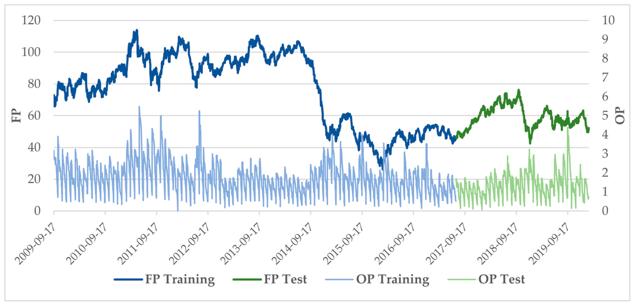
The set of observations was divided into a training set and a test set at a ratio of 75% to 25%, respectively. A continuous set of observations, starting on 17 September 2009, and ending on 14 July 2017, was chosen as the training set. The observations constituting the test set covered the period from 17 July 2017 to 14 February 2020. Figure 1 presents the chart of WTI futures prices and the value of ATM call options. The descriptive statistics for WTI futures prices, option premiums and the long call final results for the training and test sets are presented in

Table 1. Descriptive statistics of WTI futures prices, option premium and long call final results (in USD per barrel).

Category of Set	Training			Test			Total
Value	WTI Futures	Option Premium	Long Call	WTI Futures	Option Premium	Long Call	WTI Futures	Option Premium	Long Call
Number of obs.	1966			664			2630
Mean	76.92	1.7298	−0.141	59.15	1.3428	−0.1374	72.43	1.6321	−0.14
Median	83.46	1.6501	−0.8629	58.15	1.3013	−0.5246	71.54	1.5446	−0.77
Min	26.21	0.01	−5.4758	42.53	0.063	−4.3831	26.21	0.01	−5.48
Max	113.93	5.4758	12.3858	76.41	4.3831	7.5398	113.93	5.4758	12.39
Q1	51.68	1.13	−1.65	53.77	0.91	−1.33	52.76	1.04	−1.56
Q3	96.44	2.18	0.85	64.42	1.67	0.74	93.12	2.08	0.81
Std deviation	22.82	0.84	2.37	7.1	0.65	1.67	21.48	0.81	2.22
Skewness	−0.42	0.86	1.58	0.19	1	0.97	0.05	0.94	1.55
Kurtosis	−1.26	1.32	3.26	−0.72	2.19	1.48	−1.4	1.54	3.51
JB	1546.32	474.96	819.81	386.86	128.65	167.67	2062.32	620.29	1081

Notes: the training set was from 17 September 2009 to 14 July 2017; the test set was from 17 July 2017 to 14 February 2020; JB represents the Jarque–Bera test statistics for normality.

.

The presented results show that the fluctuations in both oil prices and option premiums were greater in the training set than in the test set. Moreover, mean and median values for these variables are noticeably higher in the training set. This may be a consequence of the fact that the training set covers a period of time three times longer than the test set. Negative mean values and medians for long calls show that both in the training set and the test set, the process of buying call options was much more likely to bring losses than profits (almost twice as often the purchase of ATM options generated a loss rather than a profit).

The skewness value suggests that only in the training set the oil prices have negatively skewed distributions. For option premiums and long call final results, the distribution was leptokurtic, while for WTI futures prices they were platykurtic (both for training and test set). The Jorque–Bera statistics give evidence of the non-normality of the oil price, option premium and long call results distributions for both the training and test sets.

In the next stage of empirical research, we use WTI oil prices from the analysed period to determine the following indicators:

• Standard deviation for n recent settlement prices of the WTI futures, where $n\in \left\{1, 2, 3, \dots , 9, 10, 12, 14, \dots , 28, 30, 35, 40, 45, 50, 55, 60\right\}$;
• Arithmetic mean of n recent settlements price of the WTI futures (moving average), where $n\in \left\{2, 3, \dots , 9, 10, 12, 14, \dots , 28, 30, 35, 40, 45, 50, 55, 60\right\}$.

WTI nearest futures prices and the number of days remaining until option expiry, as well as standard deviations and moving averages based on WTI futures prices, were used as input data for artificial neural networks. It should be emphasised that the role of these variables is to reflect the state of the oil market at the time of opening a long position in a call option (WTI futures price as the level of the current oil price; standard deviation as a of the dynamics of oil price changes). We also take into account the impact of the number of days remaining until option expiry as it is a parameter that has a significant impact on the level of option premiums. In turn, the moving average is widely used in technical analysis to reflect market trends. Furthermore, Dbouk et al. [57] have shown that this parameter can be used to predict the directional movement of oil prices with high accuracy.

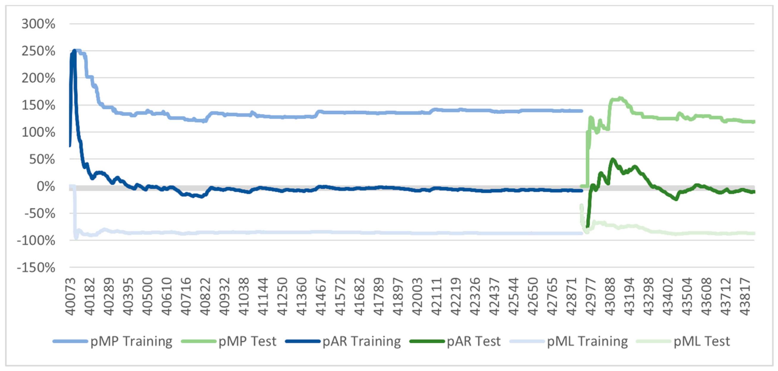
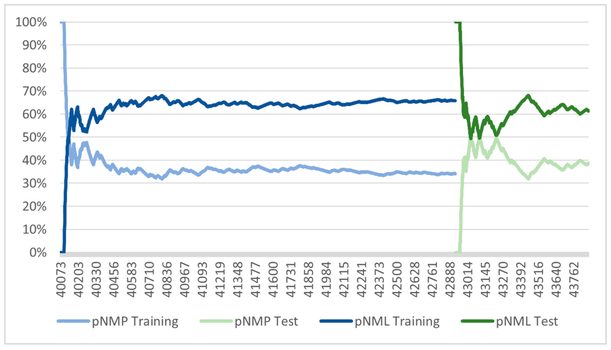
The last element presented in this part is the values of indicators such as pMP, pML, pAR (Figure 2), pNMP and pNML (Figure 3) in the training and test sets. These indicators provide information about the maximum profit, maximum loss and total sum of returns (losses) that could be achieved in the given period by taking long positions in call options. This information was used to compare the results obtained from artificial neural networks.

The values of the analysed indicators were at a similar level in the training and test sets. Moreover, there is a noticeable tendency of the pAR indicator to reach negative values quickly and not to exceed the value of 0 at the end of each of the analysed periods of time. This confirms that taking long positions in call options is much more likely to bring losses than profits, which is also shown in Figure 3.

4. Results

Next, we analysed the impact of the following parameters on the results of the network (SANN):

• The number of neurons in the hidden layer, for which three ranges were established: [5; 30], [31; 55] and [56; 80];
• Activation functions in the hidden layer: linear, logistic, exponential, sine and hyperbolic tangent;
• Activation functions in the output layer: linear, logistic, exponential, sine, hyperbolic tangent and softmax (for the joint entropy error evaluation function).

Additionally, the sum of squares and joint entropy were used as network error functions. The number of neurons in the hidden layer ranged from 5 to 80. For this study, the values of the proposed indicators for 1,000,000 networks described in [58] were recalculated and over new 1,500,000 networks were trained.

In the first part of the analysis of the results, we present the impact of such parameters as the number of neurons, and the activation functions in the output and hidden layer on %MP, pEP and pNEP indicators. The pEP indicator was used only to illustrate the ratio of the result (EP) achieved by a given network to the amount of capital needed to open positions in option contracts (the sum of option premiums). Due to the nature of the proposed study (i.e., hedging against oil price fluctuations), the pEP indicator was not used as the parameter for selecting the best networks. For %MP and pNEP indicators, the best network results were included, marked as b(%MP) and b(pNEP) respectively, where b is the function that returns the best results for a given indicator—it means ‘the best results’. It is also worth noting that since the networks were trained on the training set, the best results will also be for this set, not the test set. For comparison, the results of other indicators obtained by a given network were also included. Appendix A (

Table A1. The best results for the %MP and pNEP indicators.

Function b()	Activation Function		Number of Neurons	Training Set			Test Set
	Hidden Layer	Output Layer		%MP	pNEP	pEP	%MP	pNEP	pEP
%MP	Exp	Exp	5–30	17%	8%	84%	10%	3%	85%
%MP	Exp	Htan	5–30	18%	12%	75%	11%	2%	136%
%MP	Exp	Lin	5–30	15%	12%	62%	9%	3%	92%
%MP	Exp	Log	5–30	44%	18%	122%	18%	5%	117%
%MP	Exp	Sin	5–30	22%	14%	74%	10%	4%	74%
%MP	Exp	Smax	5–30	51%	22%	104%	12%	12%	33%
%MP	Htan	Exp	5–30	32%	17%	86%	11%	2%	124%
%MP	Htan	Htan	5–30	43%	14%	143%	21%	8%	103%
%MP	Htan	Lin	5–30	23%	14%	79%	12%	13%	48%
%MP	Htan	Log	5–30	69%	25%	128%	16%	24%	27%
%MP	Htan	Sin	5–30	32%	20%	79%	10%	25%	17%
%MP	Htan	Smax	5–30	66%	33%	98%	24%	20%	54%
%MP	Lin	Exp	5–30	2%	2%	32%	4%	1%	101%
%MP	Lin	Htan	5–30	1%	2%	29%	0%	0%	31%
%MP	Lin	Lin	5–30	2%	2%	25%	0%	1%	3%
%MP	Lin	Log	5–30	2%	2%	33%	0%	0%	31%
%MP	Lin	Sin	5–30	2%	2%	31%	0%	0%	31%
%MP	Lin	Smax	5–30	2%	5%	15%	4%	2%	50%
%MP	Log	Exp	5–30	23%	12%	83%	10%	2%	109%
%MP	Log	Htan	5–30	22%	12%	74%	8%	3%	71%
%MP	Log	Lin	5–30	22%	15%	71%	13%	7%	80%
%MP	Log	Log	5–30	66%	25%	129%	18%	28%	29%
%MP	Log	Sin	5–30	25%	15%	81%	18%	13%	57%
%MP	Log	Smax	5–30	71%	32%	104%	17%	18%	45%
%MP	Sin	Exp	5–30	10%	7%	60%	11%	3%	97%
%MP	Sin	Htan	5–30	13%	8%	69%	13%	3%	115%
%MP	Sin	Lin	5–30	9%	5%	70%	12%	3%	119%
%MP	Sin	Log	5–30	11%	7%	69%	12%	3%	101%
%MP	Sin	Sin	5–30	9%	5%	74%	10%	3%	88%
%MP	Sin	Smax	5–30	13%	5%	83%	6%	2%	70%
%MP	Exp	Exp	31–55	11%	10%	55%	8%	6%	38%
%MP	Exp	Htan	31–55	10%	11%	56%	11%	3%	111%
%MP	Exp	Lin	31–55	12%	10%	61%	14%	4%	127%
%MP	Exp	Log	31–55	32%	19%	79%	13%	2%	151%
%MP	Exp	Sin	31–55	11%	5%	81%	12%	2%	145%
%MP	Exp	Smax	31–55	42%	18%	115%	14%	4%	121%
%MP	Htan	Exp	31–55	23%	17%	60%	14%	3%	129%
%MP	Htan	Htan	31–55	10%	6%	78%	13%	2%	152%
%MP	Htan	Lin	31–55	20%	14%	61%	12%	10%	44%
%MP	Htan	Log	31–55	31%	18%	80%	10%	20%	21%
%MP	Htan	Sin	31–55	9%	7%	70%	14%	3%	136%
%MP	Htan	Smax	31–55	59%	29%	98%	17%	26%	27%
%MP	Lin	Exp	31–55	2%	2%	34%	4%	1%	141%
%MP	Lin	Htan	31–55	1%	2%	19%	0%	0%	31%
%MP	Lin	Lin	31–55	1%	2%	31%	0%	0%	31%
%MP	Lin	Log	31–55	1%	2%	24%	4%	1%	101%
%MP	Lin	Sin	31–55	2%	2%	27%	0%	1%	3%
%MP	Lin	Smax	31–55	2%	2%	29%	0%	1%	3%
%MP	Log	Exp	31–55	15%	10%	72%	11%	4%	108%
%MP	Log	Htan	31–55	11%	5%	80%	13%	2%	164%
%MP	Log	Lin	31–55	11%	8%	59%	14%	2%	163%
%MP	Log	Log	31–55	30%	20%	67%	8%	22%	18%
%MP	Log	Sin	31–55	11%	8%	68%	14%	2%	157%
%MP	Log	Smax	31–55	43%	25%	80%	11%	8%	56%
%MP	Sin	Exp	31–55	8%	3%	92%	12%	2%	132%
%MP	Sin	Htan	31–55	7%	4%	77%	10%	5%	68%
%MP	Sin	Lin	31–55	7%	3%	111%	12%	2%	151%
%MP	Sin	Log	31–55	11%	6%	77%	8%	2%	98%
%MP	Sin	Sin	31–55	5%	2%	97%	12%	2%	165%
%MP	Sin	Smax	31–55	13%	17%	33%	14%	3%	139%
%MP	Exp	Exp	56–80	9%	8%	62%	9%	2%	100%
%MP	Exp	Htan	56–80	8%	7%	67%	12%	2%	167%
%MP	Exp	Lin	56–80	11%	8%	71%	12%	3%	131%
%MP	Exp	Log	56–80	27%	14%	91%	12%	2%	145%
%MP	Exp	Sin	56–80	11%	7%	78%	11%	3%	124%
%MP	Exp	Smax	56–80	44%	20%	111%	14%	10%	50%
%MP	Htan	Exp	56–80	14%	11%	63%	13%	3%	135%
%MP	Htan	Htan	56–80	11%	6%	76%	13%	2%	164%
%MP	Htan	Lin	56–80	9%	5%	82%	13%	2%	182%
%MP	Htan	Log	56–80	38%	22%	81%	17%	27%	33%
%MP	Htan	Sin	56–80	10%	5%	85%	12%	2%	184%
%MP	Htan	Smax	56–80	37%	23%	70%	17%	30%	24%
%MP	Lin	Exp	56–80	2%	2%	32%	2%	0%	149%
%MP	Lin	Htan	56–80	2%	2%	28%	0%	0%	−42%
%MP	Lin	Lin	56–80	1%	2%	29%	0%	0%	31%
%MP	Lin	Log	56–80	2%	2%	26%	4%	1%	101%
%MP	Lin	Sin	56–80	2%	2%	27%	0%	1%	3%
%MP	Lin	Smax	56–80	2%	2%	31%	0%	1%	3%
%MP	Log	Exp	56–80	8%	6%	68%	14%	4%	114%
%MP	Log	Htan	56–80	8%	5%	64%	13%	2%	181%
%MP	Log	Lin	56–80	9%	5%	70%	14%	2%	163%
%MP	Log	Log	56–80	14%	11%	63%	14%	2%	163%
%MP	Log	Sin	56–80	8%	5%	86%	14%	3%	128%
%MP	Log	Smax	56–80	36%	23%	73%	18%	25%	36%
%MP	Sin	Exp	56–80	3%	3%	62%	5%	2%	106%
%MP	Sin	Htan	56–80	4%	3%	66%	10%	6%	59%
%MP	Sin	Lin	56–80	4%	4%	43%	8%	3%	71%
%MP	Sin	Log	56–80	9%	4%	81%	10%	3%	88%
%MP	Sin	Sin	56–80	3%	2%	70%	8%	4%	70%
%MP	Sin	Smax	56–80	8%	4%	91%	9%	4%	68%
pNEP	Exp	Exp	5–30	6%	15%	19%	12%	2%	163%
pNEP	Exp	Htan	5–30	17%	16%	53%	12%	6%	75%
pNEP	Exp	Lin	5–30	10%	15%	32%	9%	7%	43%
pNEP	Exp	Log	5–30	25%	21%	56%	4%	5%	29%
pNEP	Exp	Sin	5–30	−22%	91%	−12%	38%	41%	45%
pNEP	Exp	Smax	5–30	22%	29%	37%	11%	6%	65%
pNEP	Htan	Exp	5–30	27%	18%	63%	4%	6%	28%
pNEP	Htan	Htan	5–30	20%	17%	52%	13%	2%	134%
pNEP	Htan	Lin	5–30	15%	16%	43%	10%	19%	25%
pNEP	Htan	Log	5–30	43%	28%	69%	5%	24%	9%
pNEP	Htan	Sin	5–30	32%	20%	79%	10%	25%	17%
pNEP	Htan	Smax	5–30	66%	33%	98%	24%	20%	54%
pNEP	Lin	Exp	5–30	1%	3%	11%	1%	1%	37%
pNEP	Lin	Htan	5–30	0%	3%	2%	3%	1%	99%
pNEP	Lin	Lin	5–30	1%	3%	11%	0%	1%	3%
pNEP	Lin	Log	5–30	−1%	3%	−12%	5%	1%	114%
pNEP	Lin	Sin	5–30	1%	3%	16%	0%	1%	3%
pNEP	Lin	Smax	5–30	2%	5%	15%	4%	2%	50%
pNEP	Log	Exp	5–30	14%	18%	35%	13%	2%	149%
pNEP	Log	Htan	5–30	13%	15%	35%	10%	2%	128%
pNEP	Log	Lin	5–30	14%	15%	37%	6%	1%	114%
pNEP	Log	Log	5–30	49%	28%	87%	19%	31%	29%
pNEP	Log	Sin	5–30	9%	16%	30%	5%	5%	40%
pNEP	Log	Smax	5–30	70%	33%	103%	12%	30%	18%
pNEP	Sin	Exp	5–30	10%	9%	47%	10%	3%	90%
pNEP	Sin	Htan	5–30	13%	8%	69%	13%	3%	115%
pNEP	Sin	Lin	5–30	6%	9%	38%	8%	4%	63%
pNEP	Sin	Log	5–30	11%	7%	69%	12%	3%	101%
pNEP	Sin	Sin	5–30	5%	9%	31%	11%	3%	92%
pNEP	Sin	Smax	5–30	7%	11%	34%	10%	5%	60%
pNEP	Exp	Exp	31–55	7%	11%	39%	9%	5%	58%
pNEP	Exp	Htan	31–55	10%	11%	56%	11%	3%	111%
pNEP	Exp	Lin	31–55	8%	12%	36%	12%	5%	73%
pNEP	Exp	Log	31–55	32%	19%	79%	13%	2%	151%
pNEP	Exp	Sin	31–55	−13%	77%	−8%	46%	47%	43%
pNEP	Exp	Smax	31–55	25%	24%	52%	16%	6%	86%
pNEP	Htan	Exp	31–55	23%	17%	60%	14%	3%	129%
pNEP	Htan	Htan	31–55	6%	6%	54%	11%	5%	88%
pNEP	Htan	Lin	31–55	20%	14%	61%	12%	10%	44%
pNEP	Htan	Log	31–55	27%	20%	58%	10%	20%	19%
pNEP	Htan	Sin	31–55	5%	9%	30%	13%	4%	109%
pNEP	Htan	Smax	31–55	59%	29%	98%	17%	26%	27%
pNEP	Lin	Exp	31–55	2%	3%	20%	4%	1%	115%
pNEP	Lin	Htan	31–55	1%	2%	18%	0%	0%	31%
pNEP	Lin	Lin	31–55	1%	2%	15%	0%	1%	3%
pNEP	Lin	Log	31–55	1%	2%	24%	4%	1%	101%
pNEP	Lin	Sin	31–55	1%	3%	11%	0%	1%	3%
pNEP	Lin	Smax	31–55	0%	3%	5%	0%	1%	3%
pNEP	Log	Exp	31–55	14%	13%	42%	13%	2%	149%
pNEP	Log	Htan	31–55	8%	10%	44%	14%	2%	148%
pNEP	Log	Lin	31–55	10%	9%	55%	14%	2%	159%
pNEP	Log	Log	31–55	29%	21%	63%	3%	15%	9%
pNEP	Log	Sin	31–55	−2%	28%	−4%	34%	42%	42%
pNEP	Log	Smax	31–55	43%	25%	80%	11%	8%	56%
pNEP	Sin	Exp	31–55	7%	5%	67%	12%	4%	100%
pNEP	Sin	Htan	31–55	7%	4%	77%	10%	5%	68%
pNEP	Sin	Lin	31–55	7%	3%	111%	12%	2%	151%
pNEP	Sin	Log	31–55	6%	7%	43%	11%	5%	74%
pNEP	Sin	Sin	31–55	4%	4%	52%	12%	5%	89%
pNEP	Sin	Smax	31–55	13%	17%	33%	14%	3%	139%
pNEP	Exp	Exp	56–80	−7%	15%	−27%	20%	11%	98%
pNEP	Exp	Htan	56–80	8%	7%	67%	12%	2%	167%
pNEP	Exp	Lin	56–80	6%	10%	33%	8%	3%	89%
pNEP	Exp	Log	56–80	22%	17%	70%	11%	3%	150%
pNEP	Exp	Sin	56–80	−5%	31%	−9%	38%	57%	30%
pNEP	Exp	Smax	56–80	37%	23%	72%	18%	4%	128%
pNEP	Htan	Exp	56–80	14%	11%	63%	13%	3%	135%
pNEP	Htan	Htan	56–80	11%	6%	76%	13%	2%	164%
pNEP	Htan	Lin	56–80	9%	5%	82%	13%	2%	182%
pNEP	Htan	Log	56–80	38%	22%	81%	17%	27%	33%
pNEP	Htan	Sin	56–80	6%	6%	53%	8%	3%	111%
pNEP	Htan	Smax	56–80	36%	24%	67%	19%	26%	33%
pNEP	Lin	Exp	56–80	1%	3%	9%	0%	0%	−42%
pNEP	Lin	Htan	56–80	0%	3%	6%	0%	0%	−42%
pNEP	Lin	Lin	56–80	1%	3%	17%	0%	1%	3%
pNEP	Lin	Log	56–80	2%	2%	26%	4%	1%	101%
pNEP	Lin	Sin	56–80	2%	2%	27%	0%	1%	3%
pNEP	Lin	Smax	56–80	1%	4%	9%	0%	1%	6%
pNEP	Log	Exp	56–80	8%	6%	68%	14%	4%	114%
pNEP	Log	Htan	56–80	8%	6%	65%	12%	2%	159%
pNEP	Log	Lin	56–80	8%	7%	59%	14%	3%	131%
pNEP	Log	Log	56–80	12%	12%	45%	13%	3%	123%
pNEP	Log	Sin	56–80	−5%	31%	−9%	35%	59%	27%
pNEP	Log	Smax	56–80	36%	23%	73%	18%	25%	36%
pNEP	Sin	Exp	56–80	3%	3%	62%	5%	2%	106%
pNEP	Sin	Htan	56–80	4%	3%	66%	10%	6%	59%
pNEP	Sin	Lin	56–80	4%	4%	43%	8%	3%	71%
pNEP	Sin	Log	56–80	5%	6%	42%	11%	5%	84%
pNEP	Sin	Sin	56–80	3%	3%	60%	10%	3%	106%
pNEP	Sin	Smax	56–80	6%	6%	54%	9%	3%	109%

) summarises all the best results for the %MP and pNEP indicators, classified on the basis of the listed network parameters, i.e., the number of neurons and activation functions in the output and hidden layers.

In the figures, we used the following abbreviated names for activation functions:

• Exp—exponential,
• HTan—hyperbolic tangent,
• Lin—linear,
• Log—logistic,
• Sin—sine,
• Smax—softmax.

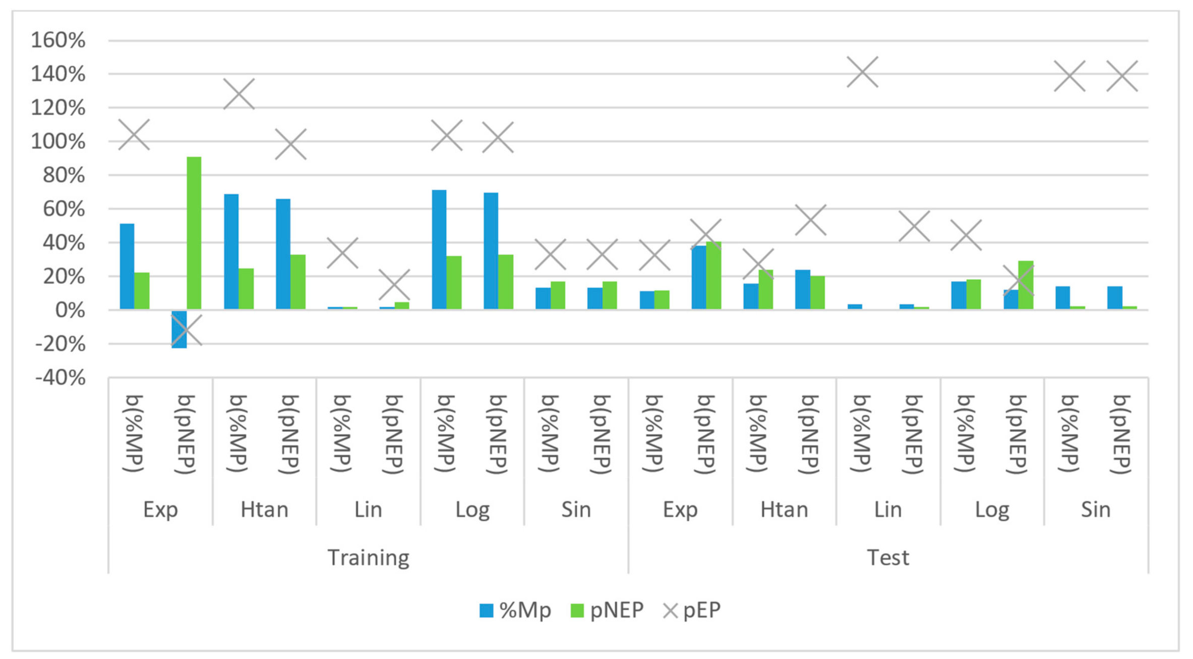
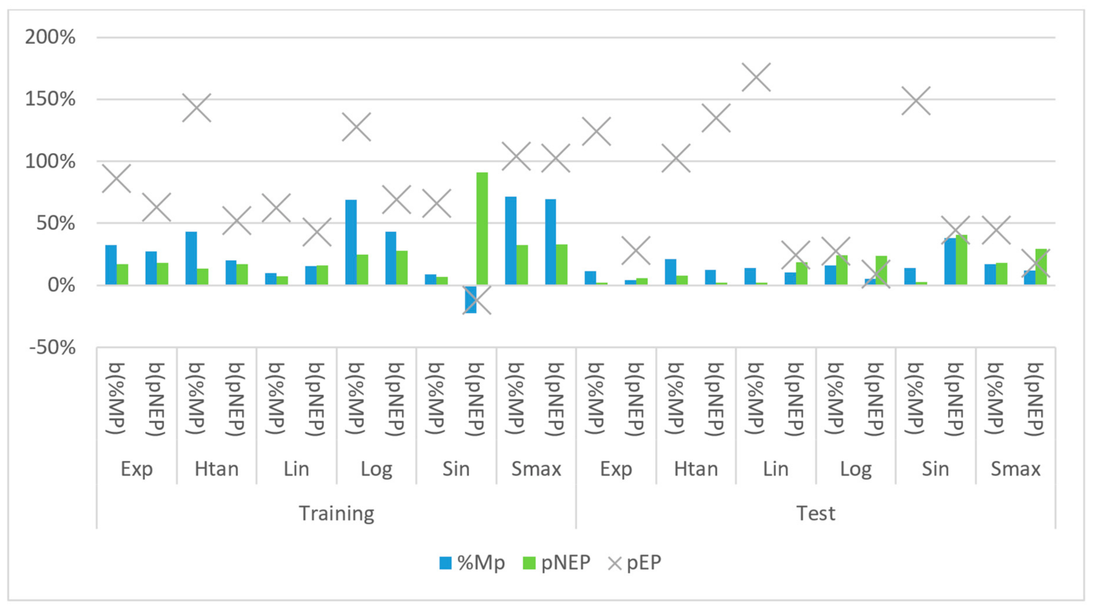
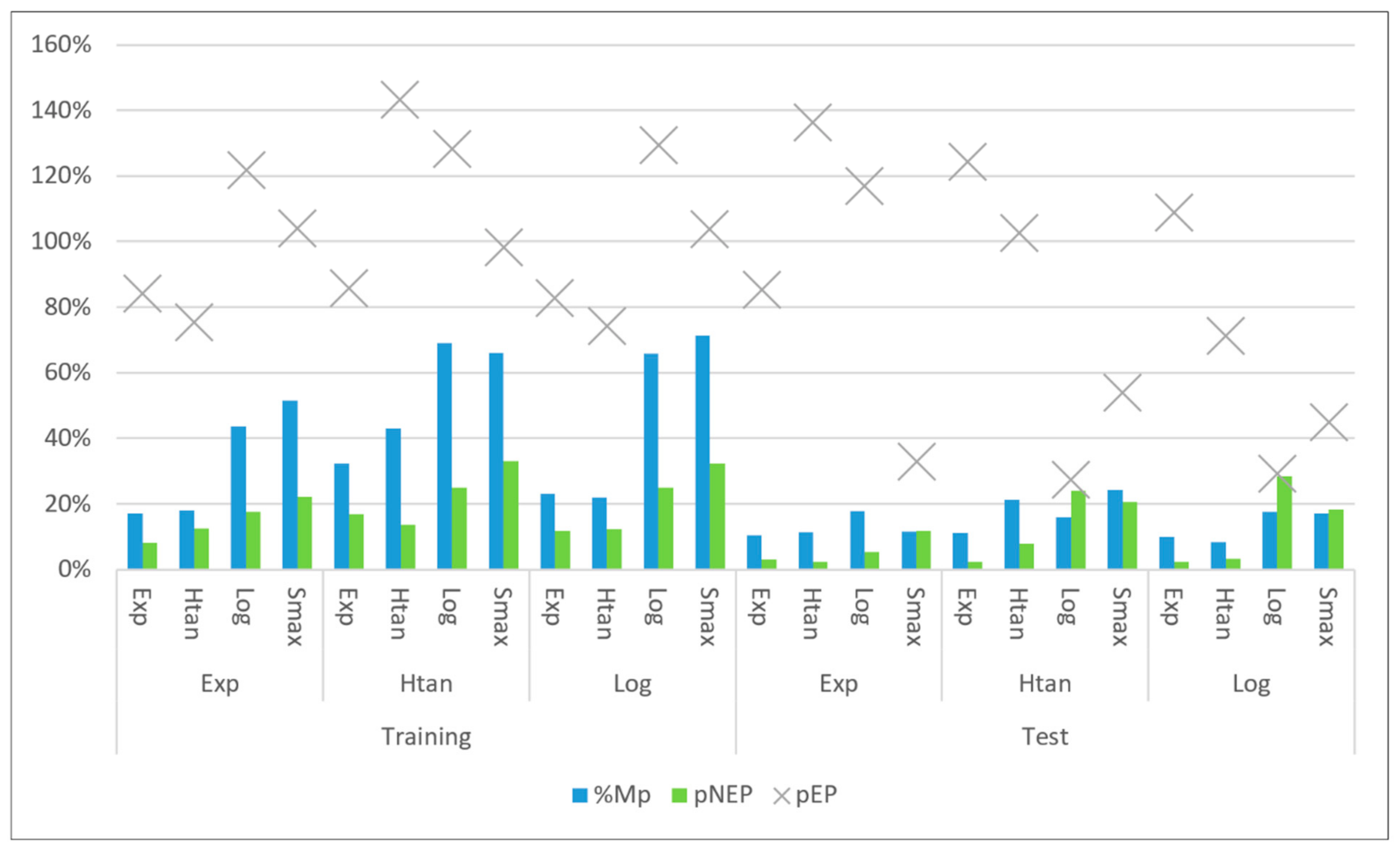
Figure 4, Figure 5 and Figure 6 show the impact of network parameters such as the number of neurons, activation functions in the output and hidden layer on the values of %MP, pEP, and pNEP indicators. For all the values of each parameter, we presented the values of two networks, namely those that allowed us to obtain the best result for the %MP indicator (b(%MP)) and for the pNEP indicator (b(pNEP)) in the training set.

Based on Figure 4, it should be noted that for both the %MP and pNEP indicators, the highest values were obtained for exponential, hyperbolic tangent and logistic activation functions in the hidden layer. The obtained rate of return was lower than zero (which is also referred to as a negative value of the pEP index for this network) only in the case of maximising the value of the pNEP index for the exponential activation function. Moreover, all these networks, defined as the best from the perspective of the training set, achieved positive values of the %MP and pEP indicators in the test set.

For activation functions in the output layer, and for the %MP indicator, the best results were achieved for the following functions: exponential, hyperbolic tangent, logistic and softmax. In the case of the pNEP index, the list of activation functions that gives the best results should also include the sine function, for which the pNEP index had by far the highest value.

The %MP indicator achieved by far the best values for the neural network for which the number of neurons ranged from 5 to 30. In terms of the pNEP indicator, we also checked networks in which the number of neurons in the hidden layer ranged from 31 to 55.

Figure 7, Figure 8 and Figure 9 present the overall analysis concerning the selection of network parameters that gave the best network results for the %MP (Figure 7) and pNEP (Figure 8 and Figure 9) indicators.

A detailed list of results that were the source for data presented in Figure 7 is attached in

Table 2. The values of %MP, pNEP and pEP indicators, depending on the type of activation function in the hidden layer and the output layer for the number of neurons in the range from 5 to 30.

Num.	Activation Function		Training			Test
	Hidden Layer	Output Layer	%MP	pNEP	pEP	%MP	pNEP	pEP
1	Exp	Exp	17.1%	8.1%	84.2%	10.4%	3.0%	85.4%
2		Htan	18.1%	12.4%	75.4%	11.4%	2.4%	136.3%
3		Log	43.7%	17.7%	121.8%	17.8%	5.4%	116.9%
4		Smax	51.4%	22.3%	104.1%	11.5%	11.9%	32.9%
5	Htan	Exp	32.4%	16.9%	85.8%	11.2%	2.4%	124.2%
6		Htan	43.1%	13.6%	143.2%	21.3%	8.0%	102.8%
7		Log	69.0%	24.9%	128.1%	15.9%	24.1%	27.4%
8		Smax	66.0%	33.1%	98.3%	24.2%	20.5%	54.0%
9	Log	Exp	23.1%	11.9%	82.7%	10.0%	2.4%	108.7%
10		Htan	21.9%	12.2%	74.1%	8.4%	3.2%	71.2%
11		Log	65.9%	24.9%	129.3%	17.6%	28.5%	29.2%
12		Smax	71.4%	32.3%	103.9%	17.1%	18.2%	44.7%

.

The highest levels of %MP indicator for the training set were obtained for the hyperbolic tangent activation function in the hidden layer with the logistic activation function in the output layer (69%), and logistic function with softmax (71.4%). Additionally, the highest values of the pNEP index were achieved for hyperbolic tangent with softmax (33.1%) and logistic with softmax (32.3%) activation functions.

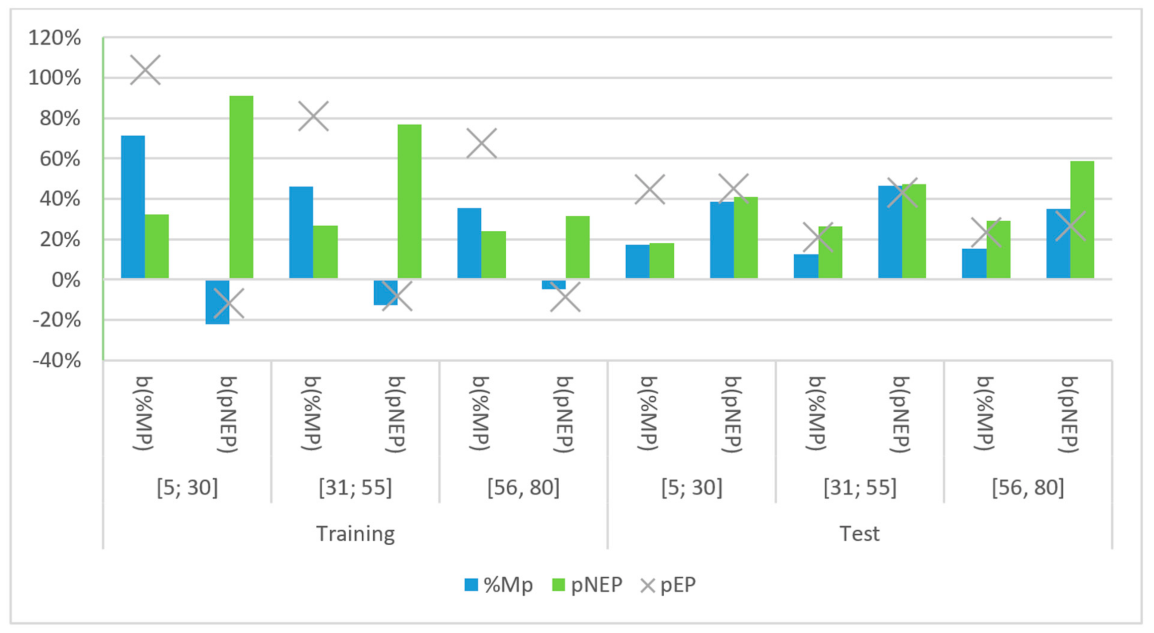
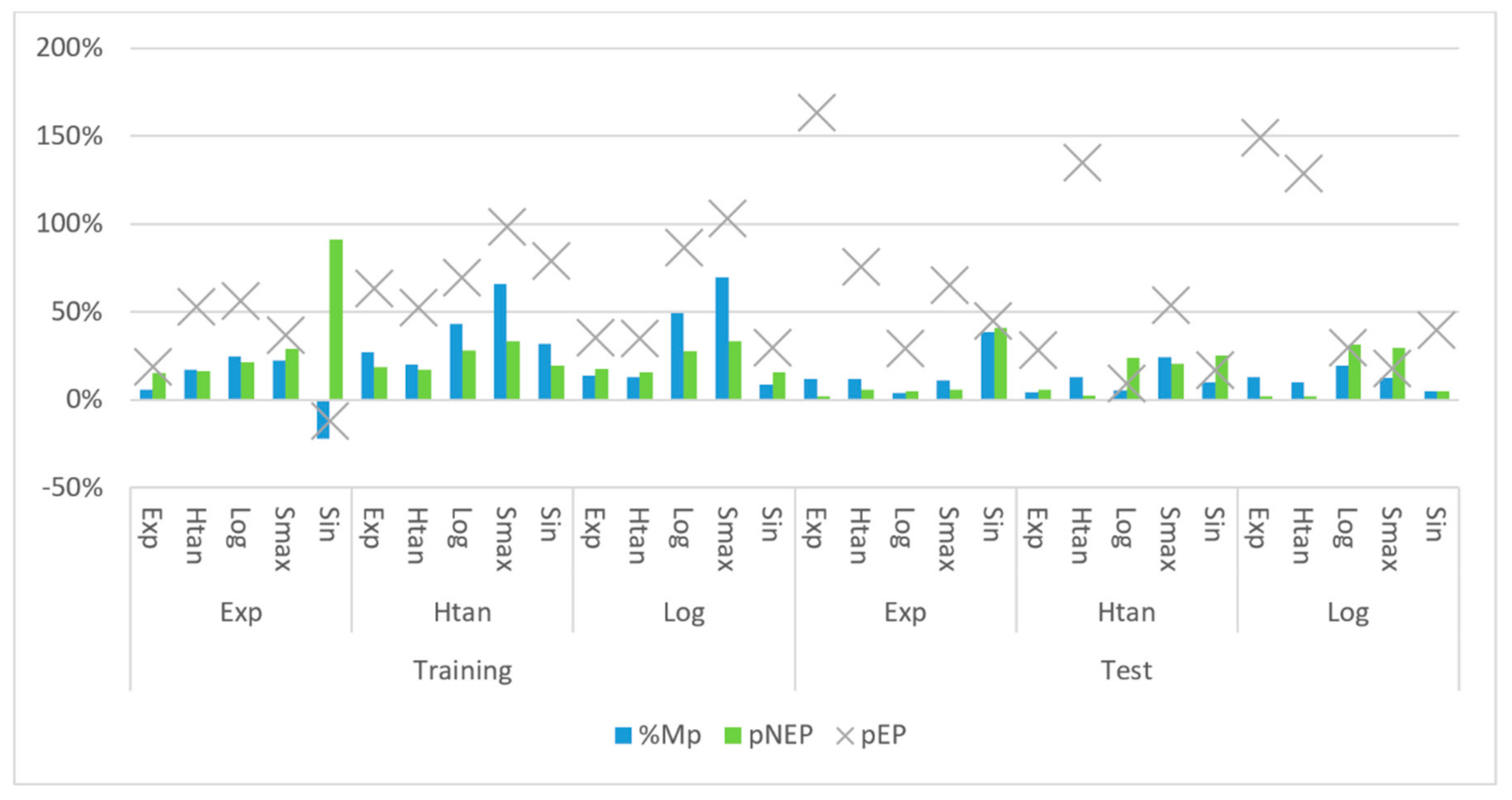
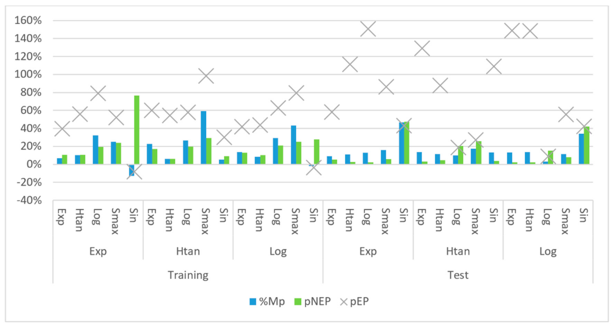
Figure 8 and Figure 9 present the best networks in terms of the value of the pNEP indicator (selected in accordance with the previously presented approach). Figure 8 shows the networks for the number of neurons in the range [5; 30], while Figure 9 depicts a summary for the number of neurons in the range [31; 55].

Table 3. List for the best neural networks based on the maximisation of pNEP indicator.

Number	Number of Neurons	Activation Function		Training			Test
		Hidden Layer	Output Layer	%MP	pNEP	pEP	%MP	pNEP	pEP
1	5–30	Exp	Exp	5.6%	15.3%	18.9%	12,00%	1.8%	163.2%
2			Htan	17.0%	15.9%	53.00%	11.6%	5.9%	75.4%
3			Log	24.5%	21.3%	56.3%	4.00%	5.00%	29.1%
4			Sin	−22.3%	91.1%	−11.9%	38.4%	40.8%	45.0%
5			Smax	22.2%	28.9%	36.6%	11.1%	5.9%	65.2%
6		Htan	Exp	27.1%	18.3%	63.0%	4.1%	5.6%	28.3%
7			Htan	20.0%	17.0%	52.3%	12.6%	2.4%	134.5%
8			Log	43.1%	28.1%	69.3%	5.2%	23.6%	9.2%
9			Sin	31.9%	19.6%	79.2%	9.8%	25.2%	16.8%
10			Smax	66.0%	33.1%	98.3%	24.2%	20.5%	54.0%
11		Log	Exp	13.7%	17.5%	35.1%	12.7%	2.1%	149.1%
12			Htan	12.7%	15.4%	34.8%	10.2%	2.1%	128.2%
13			Log	49.2%	27.7%	86.5%	19.3%	31.2%	29.5%
14			Sin	8.6%	15.6%	29.7%	4.8%	4.8%	39.5%
15			Smax	69.7%	33.1%	102.6%	12.1%	29.5%	17.7%
16	31–55	Exp	Exp	7.0%	10.7%	39.3%	9.0%	5.4%	58.2%
17			Htan	10.1%	10.7%	55.9%	11.2%	2.7%	111.4%
18			Log	32.4%	19.2%	79.1%	12.8%	2.1%	150.7%
19			Sin	−12.8%	76.7%	−8.2%	46.5%	47.3%	43.1%
20			Smax	25.0%	24.1%	52.4%	15.8%	5.6%	86.3%
21		Htan	Exp	22.6%	16.9%	60.1%	13.6%	3.00%	129.1%
22			Htan	6.0%	6.1%	54.3%	11.2%	4.5%	87.9%
23			Log	26.5%	19.7%	57.9%	9.7%	20.3%	18.7%
24			Sin	5.3%	9.1%	29.7%	13.3%	3.6%	109.0%
25			Smax	59.0%	29.1%	98.0%	17.3%	25.8%	27.1%
26		Log	Exp	13.6%	13.1%	41.9%	13.4%	2.3%	148.6%
27			Htan	8.2%	10.1%	43.7%	13.6%	2.4%	148.4%
28			Log	29.2%	20.8%	62.7%	3.1%	15.1%	8.9%
29			Sin	−1.8%	27.6%	−3.7%	34.2%	42.0%	42.1%
30			Smax	43.1%	24.9%	79.7%	11.3%	8.1%	55.6%

below presents a summary of the data used to prepare Figure 8 and Figure 9.

Significantly, the best results for the pNEP indicator were obtained with the use of the exponential activation function in the hidden layer and the sine activation function in the output layer (91.1% for 5–30 neurons and 76.7% for 31–55 neurons). The results presented in Table 3 show that the sine activation function in the output layer was the only function that returned negative %MP values for the training set. Such a relationship can be observed both in the case of the two previously indicated combinations, as well as the logistic and the sine function (with 31–55 neurons). Similarly, the use of sine function in the output layer resulted in the highest %MP values for the test set (38.4% for 5–30 neurons with the exponential function, 46.5% for 31–55 neurons with the exponential function and 34.2% for 31–55 neurons with the logistic function). Crucially, the %MP indicators for the test set for these three networks are much higher than for the networks that were chosen based on the highest b(%MP) values.

Networks with hyperbolic tangent or logistic activation functions in the hidden layer, and logistic or softmax activation functions in the output layer are considered.

As shown in Figure 8 and Figure 9, the highest values of %MP and pNEP indicators for various parameters (activation functions in the hidden layer and the output layer, number of neurons in the hidden layer) are correlated. This aspect is analysed in the next part of the study.

4.1. Correlation Analysis

The correlation between %MP and pNEP indicators is shown in

Table 4. The values of linear correlation coefficients for neural network assessment indicators (%MP and pNEP).

Number	Category		Correlation Coefficient
1	Training		−0.392
	Test		0.759
2	b(%MP)		0.694
	b(pNEP)		−0.293
3	Training	b(%MP)	0.902
	Test	b(%MP)	0.391
	Training	b(pNEP)	−0.572
	Test	b(pNEP)	0.809

Note: the bold values are statistically significant.

and Figure 4, Figure 5 and Figure 6. Correlation coefficients were calculated for three different categories. In the first, the basis for classification is the type of set for which the indicators were selected. In the second, it was the type of indicator maximisation criterion used in the hidden layer. Category 3 is a combination of categories 1 and 2.

This shows that grouping the data by training and test sample as well as selecting the ‘best’ networks, as shown by b(%MP) and b(pNEP), gives the greatest indication of the relationships between the observed results.

Following the data presented in Table 4, we conclude that there is a strong positive correlation between %MP and pNEP indicators for the training sample as reflected in a correlation coefficient of 0.902. Equally, there is no statistically significant relationship between the indicators for the test set (0.391). However, as for the maximisation of the pNEP coefficient, we notice completely different dependence, namely a moderate negative correlation for the training set. This may be the result of the negative values for the networks that use the sine as an activation function in the output layer. It is also worth noting that there is a strong correlation between the indicators for the test set, which appears to be an interesting and important phenomenon and is analysed in a further part of the study.

Due to the disadvantage of the sine function, which as the only activation function in the output layer returned negative %MP values, we decided to exclude this function in further analysis. The results are presented in

Table 5. The values of linear correlation coefficients for neural network assessment indicators (sine function excluded).

Number	Category		Correlation Coefficient
1	Training		0.945
	Test		0.546
2	b(%MP)		0.898
	b(pNEP)		0.471
3	Training	b(%MP)	0.899
	Test	b(%MP)	0.507
	Training	b(pNEP)	0.784
	Test	b(pNEP)	0.741

Note: the bold values are statistically significant.

.

Exclusion of the sine function resulted in obtaining positive correlation values for both parameters selected for both the training and test sets. For b(%MP) indicator, the correlation for the training set is significantly higher than for the test set. Whereas, for b(pNEP), the correlation between the training and test set is at a similar, high level.

Due to the discrepancy between the parameters of the best results, we decided to analyse the overall results with the use of the objective function that considers different weights of both parameters.

4.2. Network Assessment Using a Weighted Rating Function

In this part of the study, we present the results of using a weighted objective function to assess the quality of a given solution. The objective (evaluation) function (RF) has the following formula:

$$RF=a·\%MP+b·pNEP,$$

(20)

where coefficients a and b are weights of a given indicator.

The use of the presented objective function was possible due to the percentage nature of both indicators. Additionally, the following condition was added:

$$a+b=1$$

(21)

It was added to facilitate the comparison of the results obtained by the objective function and the %MP and pNEP indicators.

Investor’s preferences were analysed based on the combinations of weights presented in

Table 6. Analysed combinations of weight values.

Combination	a	b
1	0.75	0.25
2	0.5	0.5
3	0.25	0.75

. In combination 1, an investor prefers profit maximisation over the share of the number of days on which the options brought profit. Combination 3 is appropriate for investors with opposite preferences, i.e., those who place more emphasis on the number of days on which options were profitable. Whereas combination 2 puts equal weight on both parameters.

For each combination (1, 2, 3), the five highest values of the objective function are presented in

Table 7. The best results obtained for a given combination of weight values.

Comb. nr	Number of Neurons	Activation Function		Training Set			Test Set
		Hidden Layer	Output Layer	%MP	pNEP	RF	%MP	pNEP	RF
1	5–30	Log	Smax	71.4%	32.3%	61.6%	17.1%	18.2%	17.4%
	5–30	Htan	Log	69.0%	24.9%	57.9%	15.9%	24.1%	18.0%
	5–30	Htan	Smax	66.0%	33.1%	57.8%	24.2%	20.5%	23.2%
	5–30	Log	Log	65.9%	24.9%	55.6%	17.6%	28.5%	20.3%
	31–55	Htan	Smax	59.0%	29.1%	51.5%	17.3%	25.8%	19.4%
2	5–30	Log	Smax	71.4%	32.3%	51.8%	17.1%	18.2%	17.7%
	5–30	Htan	Log	69.0%	24.9%	46.9%	15.9%	24.1%	20.0%
	5–30	Htan	Smax	66.0%	33.1%	49.6%	24.2%	20.5%	22.3%
	5–30	Log	Log	65.9%	24.9%	45.4%	17.6%	28.5%	23.0%
	31–55	Tanh	Smax	59.0%	29.1%	44.1%	17.3%	25.8%	21.5%
3	5–30	Exp	Sin	−22.3%	91.1%	62.8%	38.4%	40.8%	40.2%
	31–55	Exp	Sin	−12.8%	76.7%	54.3%	46.5%	47.3%	47.1%
	5–30	Log	Smax	69.7%	33.1%	42.3%	12.1%	29.5%	25.2%
	5–30	Htan	Smax	66.0%	33.1%	41.3%	24.2%	20.5%	21.4%
	31–55	Htan	Smax	59.0%	29.1%	36.6%	17.3%	25.8%	23.6%

.

For combinations 1 and 2, the same networks gave the highest results. Two of these five networks were also included in the results for combination 3. This may be due to the high level of correlation between the %MP and pNEP indicators (see Table 5). The comparison also includes two networks with a sine activation function. They are noteworthy despite the negative result of the %MP index obtained by these networks. The networks with the sine activation function allowed us to obtain the highest RF values for both the training and test sets.

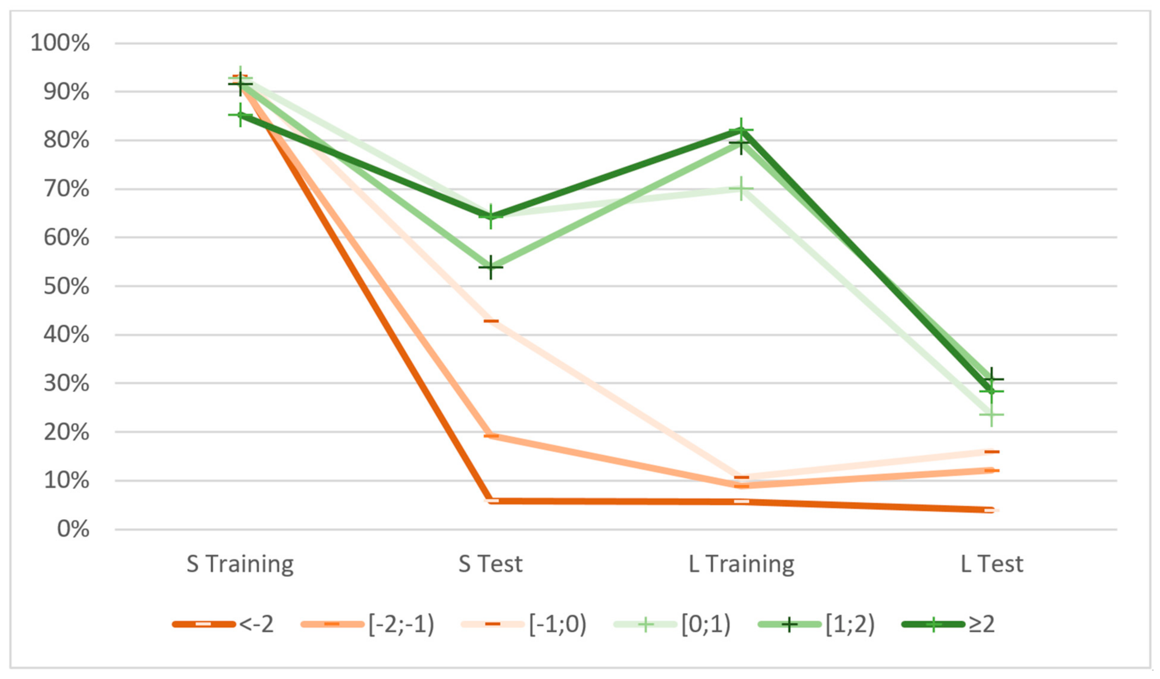
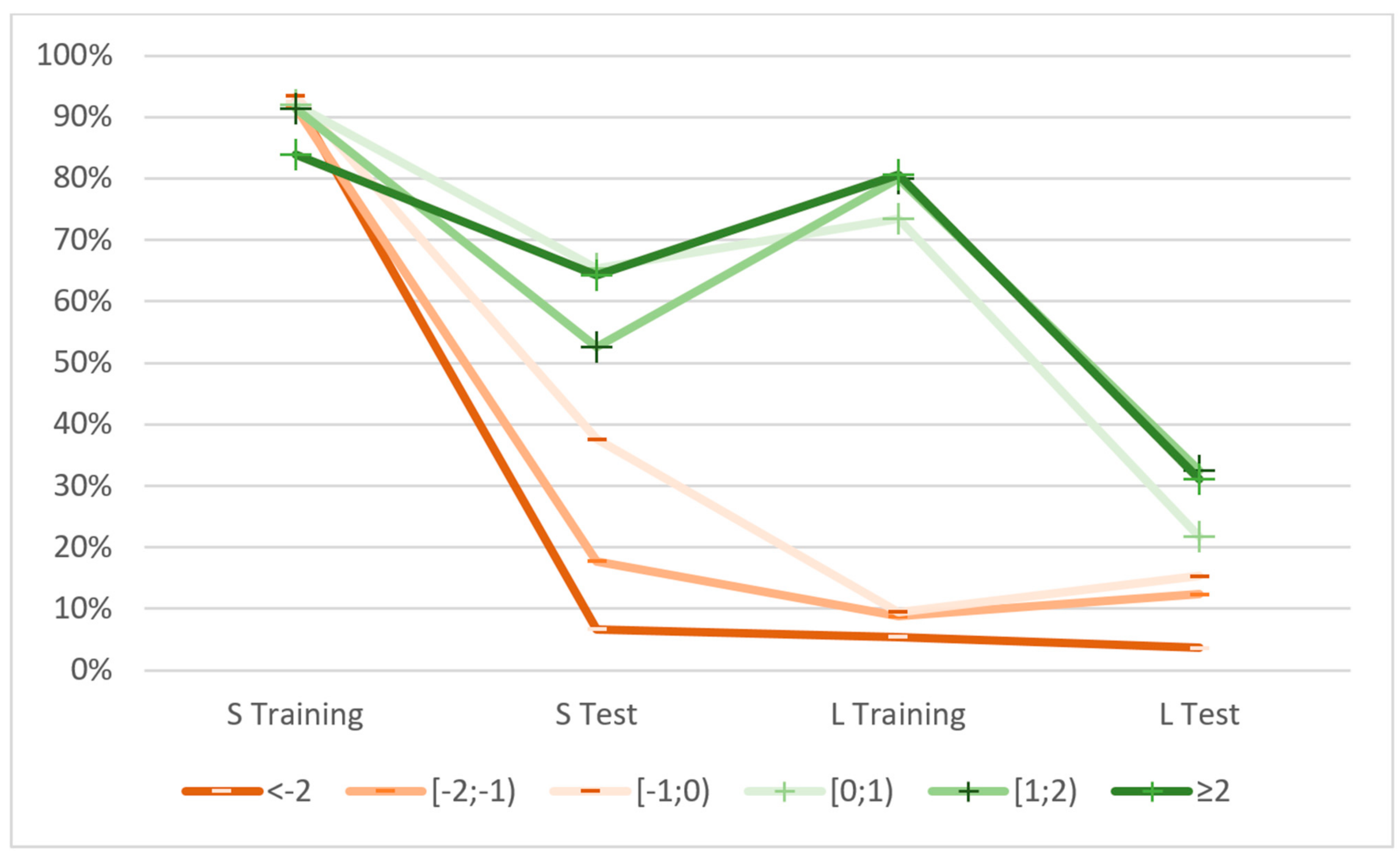
In the last stage of the comparative analysis of the results, network performance indicators for different ranges of returns from long position in call option are analysed.

4.3. Comparison of Networks Based on Effectiveness Indicators

Due to the discrepancy in the results obtained from the perspective of the %MP and pNET indicators, the authors decided to analyse the level of returns generated by networks in given value ranges (classes). For this purpose, the final results for the call option buyer (payoff) were divided into the following six classes:

• ‘<−2’: the end result from taking a long position in the call option was less than −2 USD/barrel;
• ‘[−2; −1)’: the end result from taking a long position in the call option was not less than −2 USD/barrel, but less than −1 USD/barrel;
• ‘[−1; 0)’: the end result from taking a long position in the call option was not less than −1 USD/barrel, but less than 0 USD/barrel;
• ‘[0; 1)’: the end result from taking a long position in the call option was not less than 0 USD/barrel, but less than 1 USD/barrel;
• ‘[1; 2)’: The end result from taking a long position in the call option was not less than 1 USD/barrel but less than 2 USD/barrel;
• ‘>2’: the end result from taking a long position on a call option was greater than 2 USD/barrel.

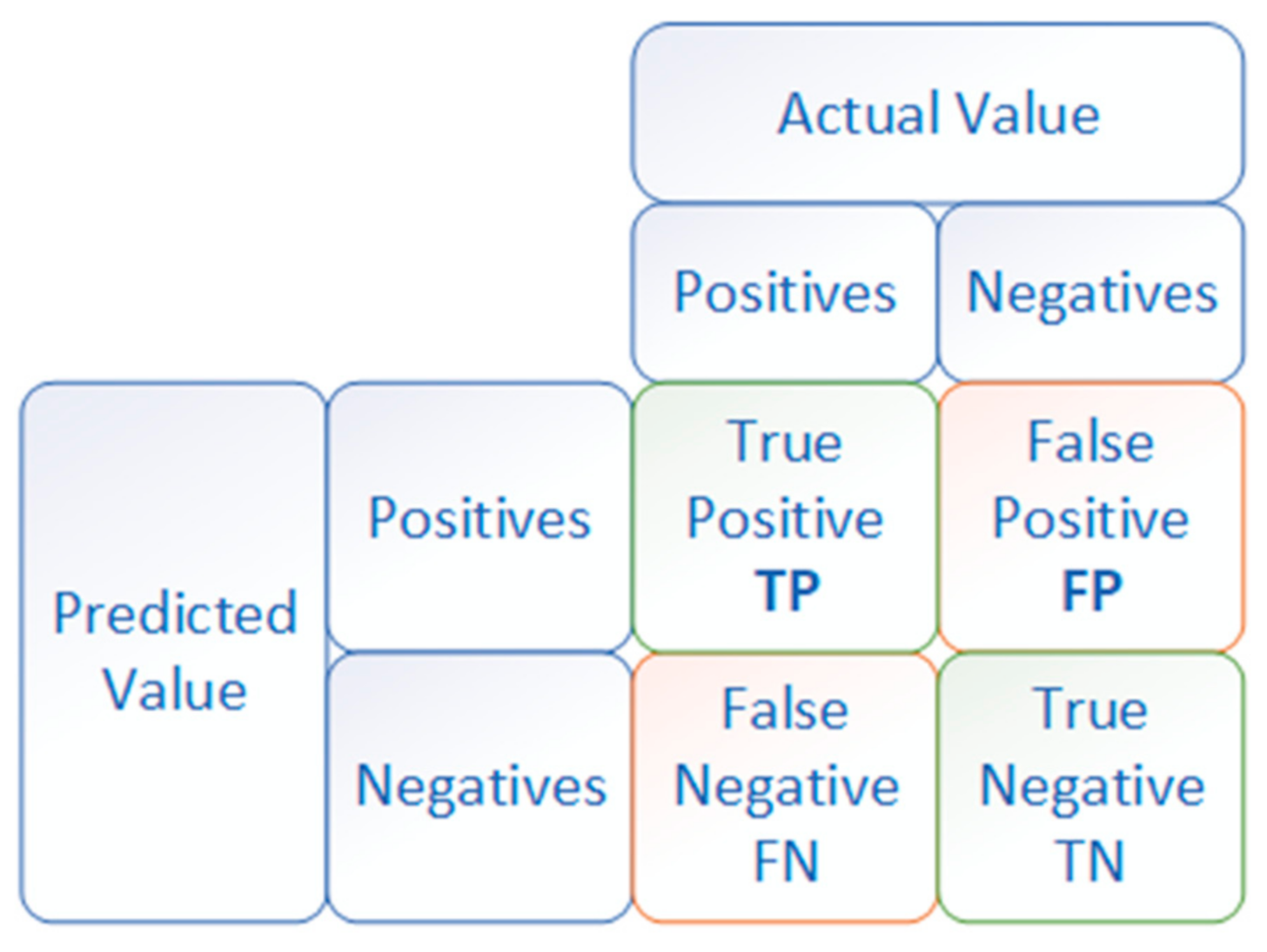
For each class, the number of options that were included in it was determined, as well as the sum of all results (payoffs) obtained from these options. Based on classes defined in this way, the networks that generated the highest values of %MP or pNEP were subjected to a detailed analysis. The confusion matrix (Figure 10) was also used to assess these networks. It shows whether the classification made as a result of the prediction was correct or incorrect (and if so what type of error was made). In the case of the problem under consideration, the main emphasis was placed on the value of ‘True Positive’, which shows the number of correctly predicted buy signals for call options, and the value of ‘False Positive’, which in turn represents the number of erroneous signals for taking a long position in the aforementioned type of option.

Among the networks, which made it possible to achieve the highest values of the pNEP indicator for the training set, the network stands out, which used a sine function as one of the activation functions (in the hidden layer or the output layer). The authors compared this group of networks with networks for which the value of the %MP indicator for the training set was the highest. Figure 11 and Figure 12 were constructed for the best networks from each of the analysed groups (based on %MP and pNEP indicators). The first one shows the ratio of the number of signals generated by a given network, which were assigned to one of the six classes, to the total number of elements in a given class (divided into training and test sets). Figure 12 shows analogous values, but in relation to the sum of the results obtained from the options (payoffs) belonging to the given classes. These values are expressed as percentage points.

As can be seen in Figure 11 and Figure 12, for both values being considered, the graphs show very similar values.

The network with a sine activation function in the output layer is characterised by a very large number of generated buy signals for the training set, both for options generating losses (ranges with values <0) and for options generating profits (ranges with values >0). This translates into very high pNEP indicators and negative %MP indicators (the vast majority of long positions in call options in the training set generated losses). At the same time, for the test set, the values of the %MP indicator increased drastically, with a very significant drop in the pNEP indicator (from 91.6% to 40.8%). This is largely due to the marked decrease in the number of buy signals generated for options that result in losses. The example of the analysed network shows the characteristic (repeating itself for the network with a sine activation function) that the number of False Positive signals is very high for the training set and it drops significantly for the test set. At the same time, the True Positive signals show much lower drops, which allows the network to achieve a very high %MP value for the test set.

In the case of the network which reached the highest value for the %MP indicator (marked with the letter L in Figure 11), the network for the training set is characterised by a very large number of profit-generating buy signals and a small number of signals that bring losses. This very high level of signals-generating profits, combined with a moderate level of signals-generating losses, translates into the highest %MP level achieved for the training set (71.5%). At the same time, this network generates moderate results for the test set (17.1%). It is worth noting that the drastic decline in this indicator is to a much lesser extent the result of an increase in the number of loss signals (False Positive) and to a much greater extent a decrease in the number of profit signals (True Positive). This tendency repeats itself for the remaining networks generating the highest values of the %MP indicator.

Based on the analyses that were conducted, it may be concluded that the main challenge for networks with sine activation functions is the excess number of buy signals generated in the test set, which bring a loss (False Positive). In the case of other networks, the problem of the buy signals being generated takes on a completely different dimension—the main challenge is the insufficient number of correct buy signals (True Positive).

5. Conclusions and Future Research Directions

Analysis of indicators related to maximum profit (MP, pMP, pNMP), maximum loss (ML, pML, pMNL) and overall results (AR, pAR) that were achieved for the period of time being considered show that it is very difficult to generate profits by buying call options. The tool proposed in the study guarantees a limited level of losses but oil prices must deviate by values exceeding the option premiums that were paid for the options to generate profits. This does diminish the effectiveness and popularity of options among the participants of various markets, such as the WTI market that was analysed in this study, as a tool designed primarily to hedge against the negative consequence of price fluctuations.

This study employs artificial neural networks to support the decision-making process of taking long position in crude oil options on the WTI market. Using the Statistica software, over 2.5 million artificial neural networks were trained for this purpose. Compared to study [58], two new indicators were proposed to assess the quality of solutions returned by the networks. The first one (pNEP) showed how often buy signals were generated in our data set. The second one (pEP) was the ratio of expected profit to the price paid for the options in a given period of time. Based on the pNEP and %MP indicators, a criterion for selecting the best networks was formulated. The results for these networks were subjected to a detailed analysis. Furthermore, the pEP index provided additional information on the rate of return obtained from these networks in relation to the level of capital employed.

The best values of the %MP indicator were obtained for networks with the smallest number of neurons (between 5 and 30) and hyperbolic tangent or logistic activation functions. On the other hand, based on this indicator, the logistic and softmax activation functions were the most effective in the output layer. For the pNEP index, ranges of 5 to 55 ([5; 30] and [31, 55]) neurons in the hidden layer of the network gave the best results. Moreover, exponential activation functions for the hidden layer and sine for the output layer were the most effective from this perspective. It is also worth noting that in the output layer only the sine activation function resulted in negative %MP values for the training set. The aforementioned indicators were used to select a network from the set of networks that were already trained. In this case, the selection criterion was the level of correctly classified buying signals from the given network which may encourage market players to take further actions or discourage them.

Excluding networks with the sine activation function resulted in a high level of correlation between the %MP and pNEP indicators. An analysis based on a weighted objective function (RF), based on %MP and pNEP indicators, confirmed a statistically significant correlation between them. The last stage of the analyses that were conducted, showed in turn, that networks with sine activation functions (in the hidden or output layers) tended to generate a large number of buy signals that brought losses in the training set. On the other hand, in the test set, the number of signals of this type showed a marked decrease—as opposed to signals generating profits. As a result, some of the networks with sine activation functions achieved very high %MP indicators of over 40% in the test set. In turn, in the case of the best networks based on the %MP indicator in the training set, large drops in %MP in the test set were caused by a significant decrease in the number of profits generating buy signals. An important characteristic of these networks was the low level of erroneously generated buy signals for both the training and test sets.

In further research, we plan to focus on improving the results from the neural networks from the perspective of their use in hedging against price risk. For this purpose, we plan to implement our own software in the field of neural networks, which will help to analyse the neural networks in detail, with regard to the various evaluation functions that may contribute to assess the network. We also plan to test different types of learning algorithms, including genetic algorithms for weighting the connections between network neurons.

References

1. Hamilton, J.D. Causes and consequences of the oil shock of 2007-08. Brook. Pap. Econ. Act. 2009, 1, 215–259. [Google Scholar] [CrossRef] [Green Version]
2. Hamilton, J.D. Oil and the macroeconomy since World War II. J. Pol. Econ. 1983, 92, 228–248. [Google Scholar] [CrossRef]
3. Hamilton, J.D. What is an oil shock? J. Econ. 2003, 113, 363–398. [Google Scholar] [CrossRef]
4. Kilian, L. Exogenous oil supply shocks: How big are they and how much do they matter for the US economy? Rev. Econ. Stat. 2008, 90, 216–240. [Google Scholar] [CrossRef]
5. Kilian, L. Not All Oil Price Shocks Are Alike: Disentangling Demand and Supply Shocks in the Crude Oil Market. Am. Econ. Rev. 2009, 99, 1053–1069. [Google Scholar] [CrossRef] [Green Version]
6. Kilian, L.; Vigfusson, R.J. Are the responses of the U.S. economy asymmetric in energy price increases and decreases? Quant. Econ. 2011, 2, 419–453. [Google Scholar] [CrossRef] [Green Version]
7. Hamilton, J.D. Nonlinearities and the macroeconomic effects of oil prices. Macroecon. Dyn. 2011, 15, 364–378. [Google Scholar] [CrossRef] [Green Version]
8. Charfeddine, L.; Klein, T.; Walther, T. Reviewing the oil price–GDP growth relationship: A replication study. Energy Econ. 2020, 88, 1–10. [Google Scholar] [CrossRef]
9. Jimenez-Rodriguez, R.; Sanchez, M. Oil price shocks and real GDP growth: Empirical evidence for some OECD countries. Appl. Econ. 2005, 37, 201–228. [Google Scholar] [CrossRef]
10. Atukeren, E. Oil price shocks and the Swiss economy: A causal investigation. Aussenwirtschaft 2005, 60, 151–168. [Google Scholar]
11. Cavalcanti, T.V.; De, V.; Mohaddes, K.; Raissi, M. Commodity Price Volatility and the Sources of Growth. J. Appl. Econ. 2014, 857–873. [Google Scholar] [CrossRef] [Green Version]
12. Jones, C.; Kaul, G. Oil and the stock markets. J. Financ. 1996, 51, 463–491. [Google Scholar] [CrossRef]
13. Basher, S.A.; Sadorsky, P. Oil price risk and emerging stock markets. Glob. Financ. J. 2006, 17, 224–251. [Google Scholar] [CrossRef]
14. Nandha, M.; Faff, R. Does oil move equity prices? A global view. Energy Econ. 2008, 30, 986–997. [Google Scholar] [CrossRef]
15. Al Rahahleh, N.; Bhatti, M.I. Co-movement measure of information transmission on international equity markets. Phys. A Stat. Mech. Appl. 2017, 470, 119–131. [Google Scholar] [CrossRef]
16. Hsiao, C.-L.; Lin, W.; Wei, X.; Yan, G.; Li, S.; Sheng, N. The Impact of International Oil Prices on the Stock Price Fluctuations of China’s Renewable Energy Enterprises. Energies 2019, 12, 4630. [Google Scholar] [CrossRef] [Green Version]
17. Zhu, J.; Song, Q.; Streimikiene, D. Multi-Time Scale Spillover Effect of International Oil Price Fluctuation on China’s Stock Markets. Energies 2020, 13, 4641. [Google Scholar] [CrossRef]
18. Wu, M.-H.; Ni, Y.-S. The effects of oil prices on inflation, interest rates and money. Energy 2011, 36, 4158–4164. [Google Scholar] [CrossRef]
19. Golub, S. Oil prices and exchange rates. Econ. J. 1983, 93, 576–593. [Google Scholar] [CrossRef]
20. Zhang, Y.J.; Fan, Y.; Tsai, H.T.; Wei, Y.M. Spillover effect of US dollar exchange rate on oil prices. J. Policy Model 2008, 30, 973–991. [Google Scholar] [CrossRef]
21. Reboredo, J.C.; Rivera-Castro, M.A. A wavelet decomposition approach to crude oil price and exchange rate dependence. Econ. Model. 2013, 32, 42–57. [Google Scholar] [CrossRef]
22. De Truchis, G.; Keddad, B. On the risk comovements between the crude oil market and U.S. dollar exchange rates. Econ. Model. 2016, 52, 206–215. [Google Scholar] [CrossRef] [Green Version]
23. Śmiech, S.; Papież, M.; Rubaszek, M.; Snarska, M. The role of oil price uncertainty shocks on oil-exporting countries. Energy Econ. 2021, 93, 105028. [Google Scholar] [CrossRef]
24. Antonakakis, N.; Chatziantoniou, I.; Filis, G. Dynamic spillovers of oil price shocks and economic policy uncertainty. Energy Econ. 2014, 44, 433–447. [Google Scholar] [CrossRef] [Green Version]
25. Ewing, B.T.; Malik, F. Volatility transmission between gold and oil futures under structural breaks. Int. Rev. Econ. Financ. 2013, 25, 113–121. [Google Scholar] [CrossRef]
26. Chen, R.; Xu, J. Forecasting volatility and correlation between oil and gold prices using a novel multivariate GAS model. Energy Econ. 2019, 78, 379–391. [Google Scholar] [CrossRef]
27. Sari, R.; Hammoudeh, S.; Soytas, U. Dynamics of oil price, precious metal prices and exchange rate. Energy Econ. 2010, 32, 351–362. [Google Scholar] [CrossRef]
28. Popp, J.; Oláh, J.; Fekete, M.F.; Lakner, Z.; Máté, D. The Relationship between Prices of Various Metals, Oil and Scarcity. Energies 2018, 11, 2392. [Google Scholar] [CrossRef] [Green Version]
29. Wu, F.; Guan, Z.; Myers, R.J. Volatility spillover effects and cross hedging in corn and crude oil futures. J. Futures Mark. 2011, 31, 1052–1075. [Google Scholar] [CrossRef]
30. Walid, M.; Shawkat, H.; Duc, K.; Seong, Y. Dynamic spillovers among major energy and cereal commodity prices. Energy Econ. 2014, 43, 225–243. [Google Scholar]
31. Taghizadeh-Hesary, F.; Rasoulinezhad, E.; Yoshino, N. Volatility Linkages between Energy and Food Prices: Case of Selected Asian Countries. Asian Development Bank Institute Working Paper 829. Available online: https://www.adb.org/sites/default/files/publication/411176/adbi-wp829.pdf (accessed on 15 April 2020).
32. Vo, D.H.; Vu, T.N.; Vo, A.T.; McAleer, M. Modeling the Relationship between Crude Oil and Agricultural Commodity Prices. Energies 2019, 12, 1344. [Google Scholar] [CrossRef] [Green Version]
33. Villar, J.A.; Joutz, F.L. The relationship between crude oil and natural gas prices. Energy Inf. Adm. Off. Oil Gas 2006, 1–43. [Google Scholar]
34. Ji, Q.; Geng, J.B.; Fan, Y. Separated influence of crude oil prices on regional natural gas import prices. Energy Policy 2014, 70, 96–105. [Google Scholar] [CrossRef]
35. Lin, B.; Li, J. The spillover effects across natural gas and oil markets: Based on the VEC–MGARCH framework. Appl. Energy 2015, 155, 229–241. [Google Scholar] [CrossRef]
36. Ji, Q.; Geng, J.B.; Aviral, K.T. Information spillovers and connectedness networks in the oil and gas markets. Energy Econ. 2018, 75, 71–84. [Google Scholar] [CrossRef]
37. Zhang, D.Y.; Shi, M.; Shi, X. Oil indexation, market fundamentals, and natural gas prices: An investigation of the Asian premium in natural gas trade. Energy Econ. 2018, 69, 33–41. [Google Scholar] [CrossRef] [Green Version]
38. Liu, C.; Sun, X.; Chen, J.; Li, J. Statistical properties of country risk ratings under oil price volatility: Evidence from selected oil-exporting countries. Energy Policy 2016, 92, 234–245. [Google Scholar] [CrossRef]
39. Sadik-Zada, E.R. Natural resources, technological progress, and economic modernization. Rev. Dev. Econ. 2021, 25, 381–404. [Google Scholar] [CrossRef]
40. Lee, C.C.; Lee, C.C.; Ning, S.L. Dynamic relationship of oil price shocks and country risks. Energy Econ. 2017, 66, 571–581. [Google Scholar] [CrossRef]
41. Lee, Y.; Yoon, S.-M. Dynamic Spillover and Hedging among Carbon, Biofuel and Oil. Energies 2020, 13, 4382. [Google Scholar] [CrossRef]
42. Zeng, S.; Jia, J.; Su, B.; Jiang, C.; Zeng, G. The volatility spillover effect of the European Union (EU) carbon financial market. J. Clean. Prod. 2021, 282, 124394. [Google Scholar] [CrossRef]
43. Wang, J.; Wang, J. Forecasting energy market indices with recurrent neural networks: Case study of crude oil price fluctuations. Energy 2016, 102, 365–374. [Google Scholar] [CrossRef]
44. Azadeh, A.; Moghaddam, M.; Khakzad, M.; Ebrahimipour, V. A flexible neural network-fuzzy mathematical programming algorithm for improvement of oil price estimation and forecasting. Comput. Ind. Eng. 2012, 62, 421–430. [Google Scholar] [CrossRef]
45. Chiroma, H.; Abdulkareem, S.; Herawan, T. Evolutionary neural network model for West Texas Intermediate crude oil price prediction. Appl. Energy 2015, 142, 266–273. [Google Scholar] [CrossRef]
46. Liu, D.; Liang, Y.; Zhang, L.; Lung, P.; Ullah, R. Implied volatility forecast and option trading strategy. Int. Rev. Econ. Financ. 2021, 71, 943–954. [Google Scholar] [CrossRef]
47. Mohamed, M.M.; El-Masry, A.A. Oil price forecasting using gene expression programming and artificial neural networks. Econ. Model. 2016, 54, 40–53. [Google Scholar]
48. Yusof, Y.; Mustaffa, Z. A review on optimization of least squares support vector machine for time series forecasting. Int. J. Artif. Intell. Appl. 2016, 7, 35–49. [Google Scholar] [CrossRef]
49. Zhao, Y.; Li, J.; Yu, L. A deep learning ensemble approach for crude oil price forecasting. Energy Econ. 2017, 66, 9–16. [Google Scholar] [CrossRef]
50. Huang, L.; Wang, J. Global crude oil price prediction and synchronization based accuracy evaluation using random wavelet neural network. Energy 2018, 151, 875–888. [Google Scholar] [CrossRef]
51. Safari, A.; Davallou, M. Oil price forecasting using a hybrid model. Energy 2018, 148, 49–58. [Google Scholar] [CrossRef]
52. Li, T.; Hu, Z.; Jia, Y.; Wu, J.; Zhou, Y. Forecasting crude oil prices using ensemble empirical mode decomposition and sparse Bayesian learning. Energies 2018, 11, 1882. [Google Scholar] [CrossRef] [Green Version]
53. Wang, M.; Zhao, L.; Ruijin, D.; Wang, C.; Lin, C.; Lixin, T.; Stanley, H.E. A novel hybrid method of forecasting crude oil prices using complex network science and artificial intelligence algorithms. Appl. Energy 2018, 220, 480–495. [Google Scholar] [CrossRef]
54. Ding, Y. A novel decompose-ensemble methodology with AIC-ANN approach for crude oil forecasting. Energy 2018, 154, 328–336. [Google Scholar] [CrossRef]
55. Li, T.; Zhou, Y.; Li, X.; Wu, J.; He, T. Forecasting daily crude oil prices using improved CEEMDAN and ridge regression-based predictors. Energies 2019, 12, 3603. [Google Scholar] [CrossRef] [Green Version]
56. Wu, J.; Miu, F.; Li, T. Daily Crude Oil Price Forecasting Based on Improved CEEMDAN, SCA, and RVFL: A Case Study in WTI Oil Market. Energies 2020, 13, 1852. [Google Scholar] [CrossRef] [Green Version]
57. Dbouk, W.; Jamali, I. Predicting daily oil prices: Linear and non-linear models. Res. Int. Bus. Financ. 2018, 46, 149–165. [Google Scholar] [CrossRef]
58. Puka, R.; Łamasz, B. Using Artificial Neural Networks to Find Buy Signals for WTI Crude Oil Call Options. Energies 2020, 13, 4359. [Google Scholar] [CrossRef]
59. Welcome to NYMEX WTI Light Sweet Crude Oil Futures. Available online: https://www.cmegroup.com/trading/why-futures/welcome-to-nymex-wti-light-sweet-crude-oil-futures.html (accessed on 15 December 2020).
60. Chapter 550. Light Sweet Crude Oil European Financial Option. Available online: https://www.cmegroup.com/content/dam/cmegroup/rulebook/NYMEX/5/550.pdf (accessed on 15 December 2020).
61. Black, F. The pricing of commodity contracts. J. Polit. Econ. 1976, 81, 167–179. [Google Scholar] [CrossRef]
62. Hull, J. Option, Futures and Other Derivatives, 8th ed.; Pearson: Boston, MA, USA, 2012. [Google Scholar]
63. Łamasz, B.; Iwaszczuk, N. Crude Oil Option Market Parameters and Their Impact on the Cost of Hedging by Long Strap Strategy. Int. J. Energy Econ. Policy 2020, 10, 471–480. [Google Scholar] [CrossRef]
64. Clark, I.J. Commodity Option Pricing: A Practioner’s Guide; Wiley Finance Series; TJ International Ltd.: Padstow, UK, 2014. [Google Scholar]
65. QuikVol Tool. WTI (LO) Volatility and Skew. Available online: https://www.cmegroup.com/tools-information/quikstrike/pricing-volatility-strategy-tools/quikvol-tool.html (accessed on 15 April 2020).
66. Peng, C.-C.; Magoulas, G.D. Nonmonotone BFGS-trained recurrent neural networks for temporal sequence processing. Appl. Math. Comput. 2011, 217, 5421–5441. [Google Scholar] [CrossRef]
Figure 1. WTI crude oil futures prices (FP) and the long call option premium (OP) for front-month delivery (in USD per barrel).
Energies 14 03308 g001
Figure 2. pMP, pML and pAR indicators over time for the training and test sets.
Energies 14 03308 g002
Figure 3. pNMP and pNML indicators over time for the training test sets.
Energies 14 03308 g003
Figure 4. The highest values of the %MP and pNEP indicators, broken down by the type of activation function in the hidden layer, from the perspective of the training set.
Energies 14 03308 g004
Figure 5. The highest values of the %MP and pNEP indicators, broken down by type of activation functions in the output layer, from the perspective of the training set.
Energies 14 03308 g005
Figure 6. The highest values of %MP, pNEP and pEP indicators, considering the number of neurons in the hidden layer.
Energies 14 03308 g006
Figure 7. The values of %MP, pNEP and pEP indicators, depending on the type of activation function in the hidden layer and the output layer for the number of neurons in the range from 5 to 30.
Energies 14 03308 g007
Figure 8. List for the best neural networks in accordance with the maximisation of pNEP indicator. Note: The number of neurons in the hidden layer ranged from 5 to 30.
Energies 14 03308 g008
Figure 9. List for the best neural networks in accordance with the maximisation of pNEP indicator. Note: The number of neurons in the hidden layer ranged from 31 to 55.
Energies 14 03308 g009
Figure 10. Confusion matrix.
Energies 14 03308 g010
Figure 11. Percentage share of the number of buy signals from the best networks (based %MP and pNEP indicators) achieved for a given class of values. Note: S is the best network based on pNEP and L based on %MP indicator.
Energies 14 03308 g011
Figure 12. Percentage share of the sum of values obtained from buy signals of the best networks (for %MP and pNEP indicators) achieved for a given value class. Note: S is the best network based on pNEP and L based on %MP indicator.
Energies 14 03308 g012