
The Impact of Energy Storage along with the Allocation of RES on the Reduction of Energy Costs Using MILP


Abstract
:1. Introduction
Novelty of the Paper
2. Problem Formulation
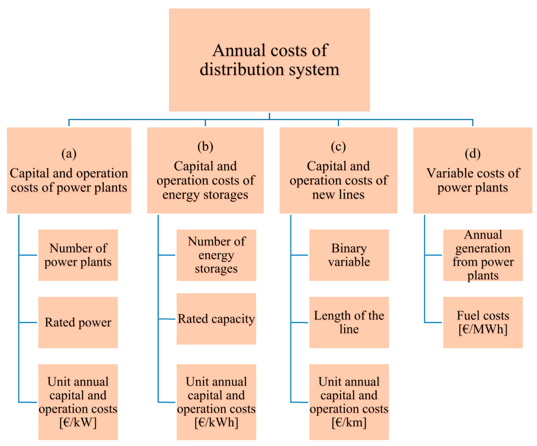
2.1. Objective Function
- Annual fixed costs of generating units;
- Annual fixed costs of energy storage;
- Operating variable costs.
2.2. Constraints
3. Assumptions
- Employee remuneration;
- Taxes;
- Equipment service;
- Insurance.
4. Simulation
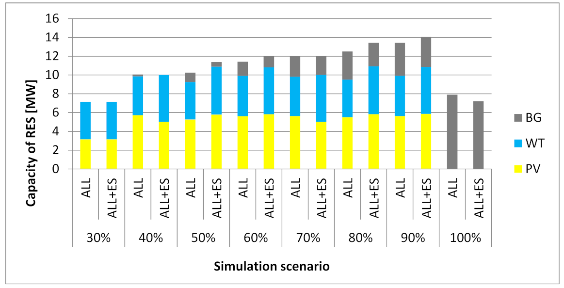
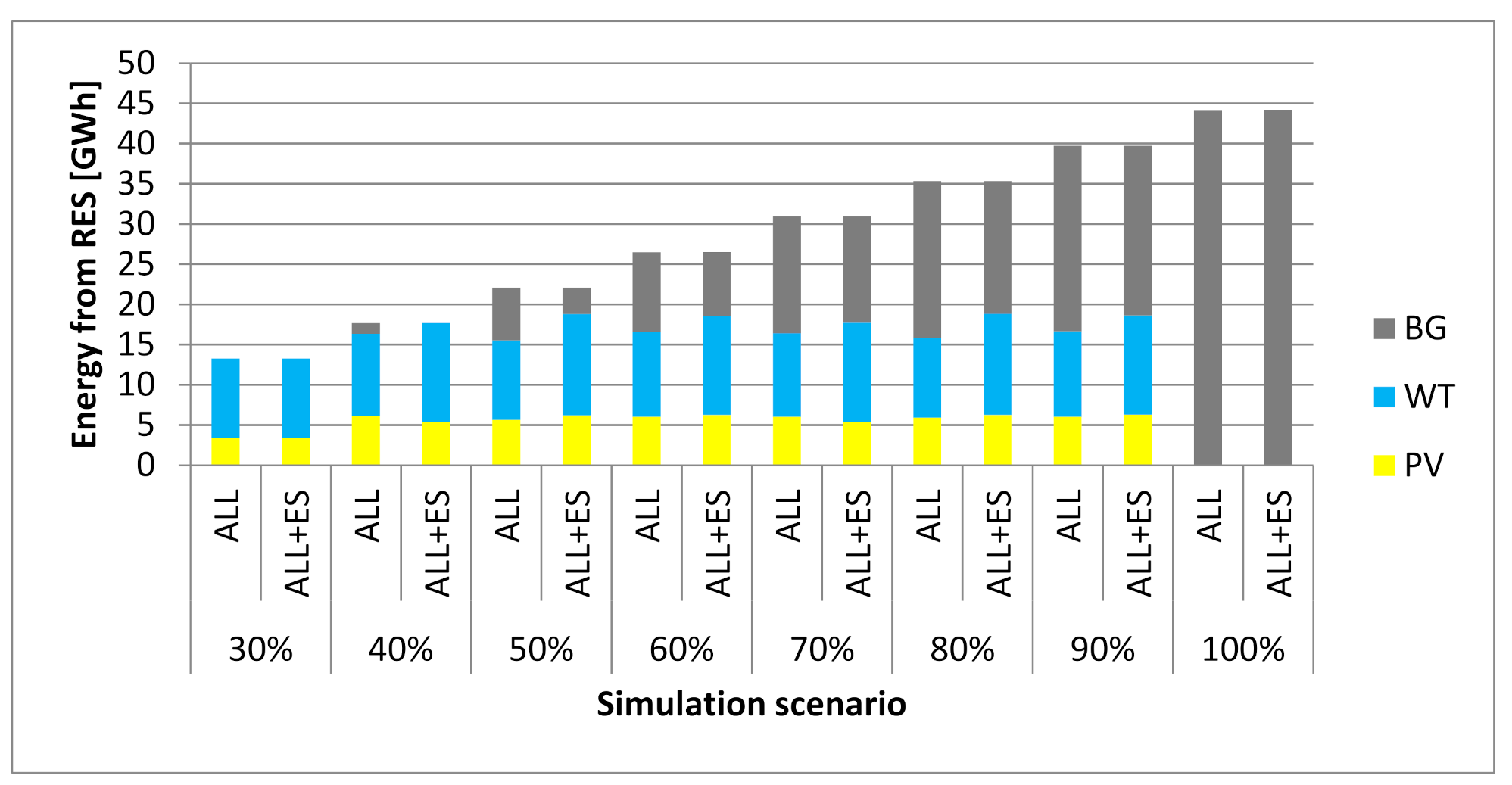
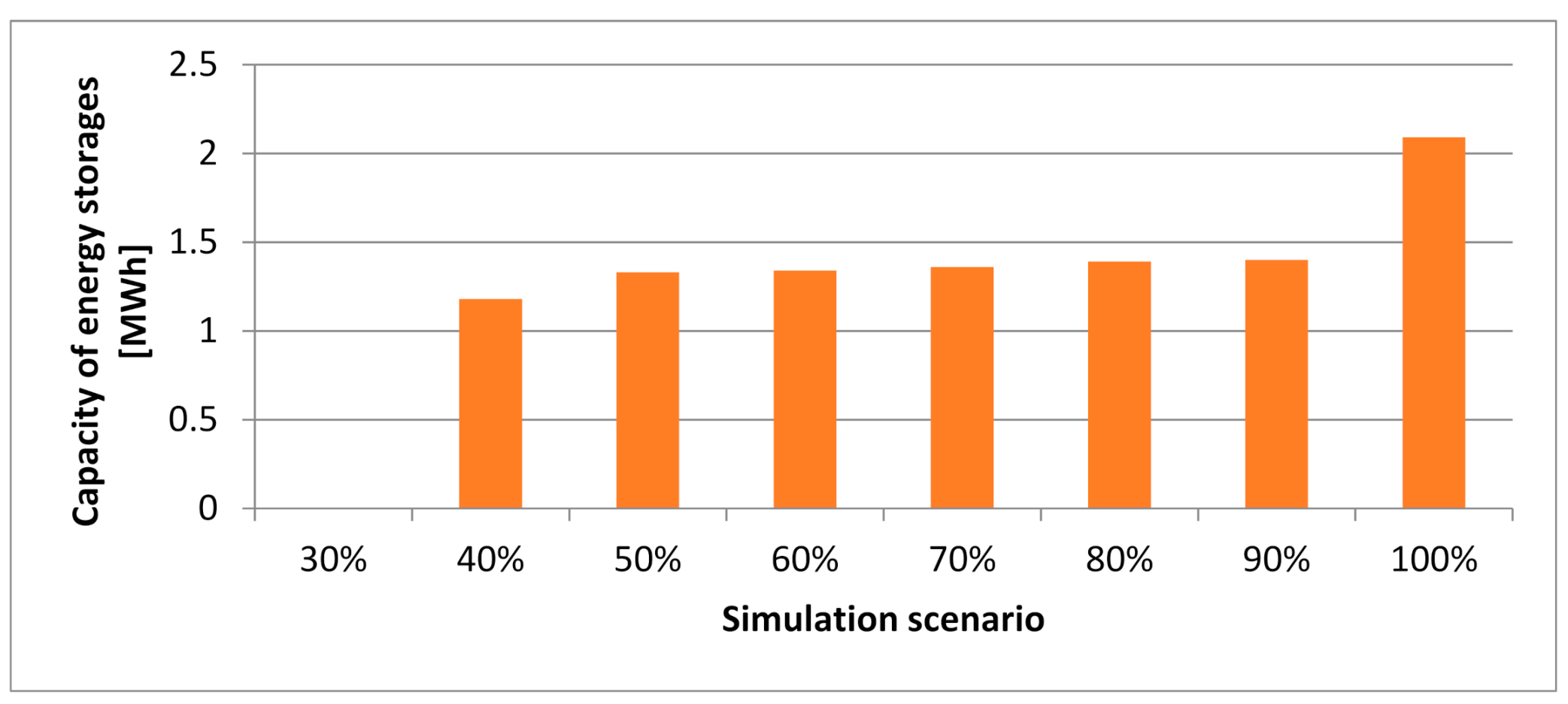
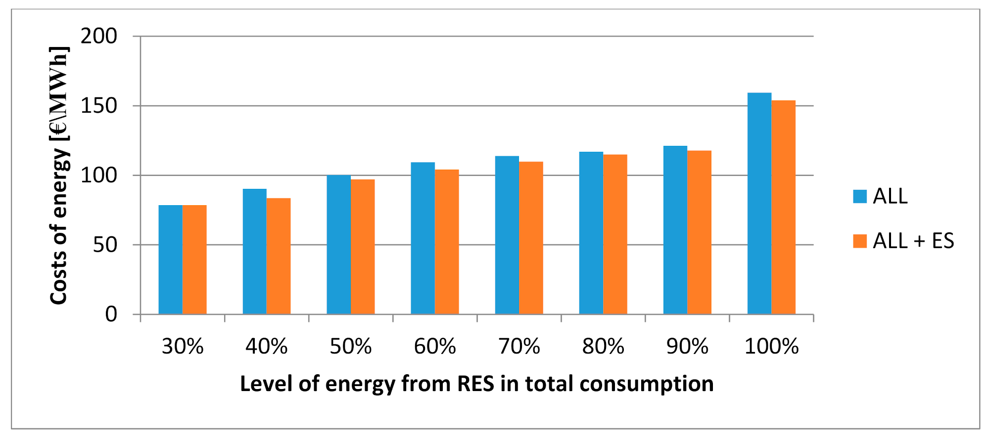
5. Results
6. Conclusions
Funding
Data Availability Statement
Acknowledgments
Conflicts of Interest
Abbreviations
| Sets | |
| n,w ∊ N | sets of indices n,w representing number of nodes in distribution network |
| d ∊ D | set of indices d representing type of Renewable Energy Sources (RES) technology—D = [d1,…d3], where d1 is the first possible technology and d3 is the last one |
| l ∊ L | set of indices l representing number of possible load type. L = [l1,…l3], where l1 is the first possible type and l3 is the last one |
| r ∊ R | set of indices r representing type of rated power for each type of possible RES technology |
| e ∊ S | set of indices d representing type energy storage |
| s ∊ S | set of indices s representing type new line that can be built in distribution system |
| Coefficients | |
| annual energy production from each type of RES r in each node n | |
| total production from RES type d in node n in time t | |
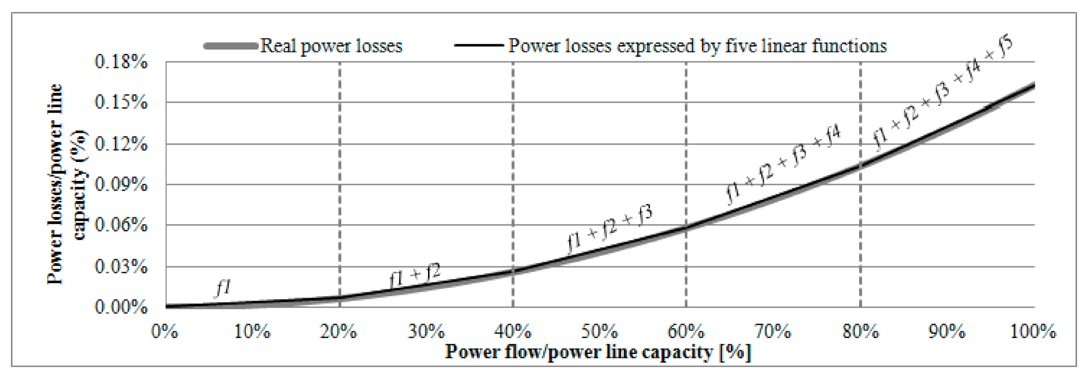
| power losses in a power line between nodes w and k in time t | |
| rated power of RES technology d for the power unit series type r | |
| total energy from RES type d in node n in time step t | |
| nominal capacity of single energy storage of type e | |
| distance between nodes “n” and “w” | |
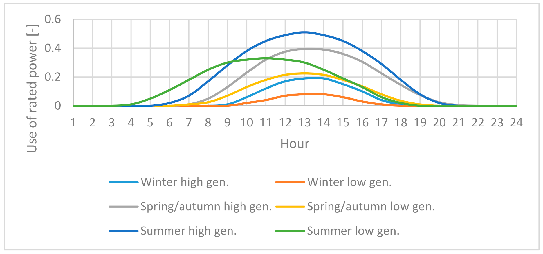
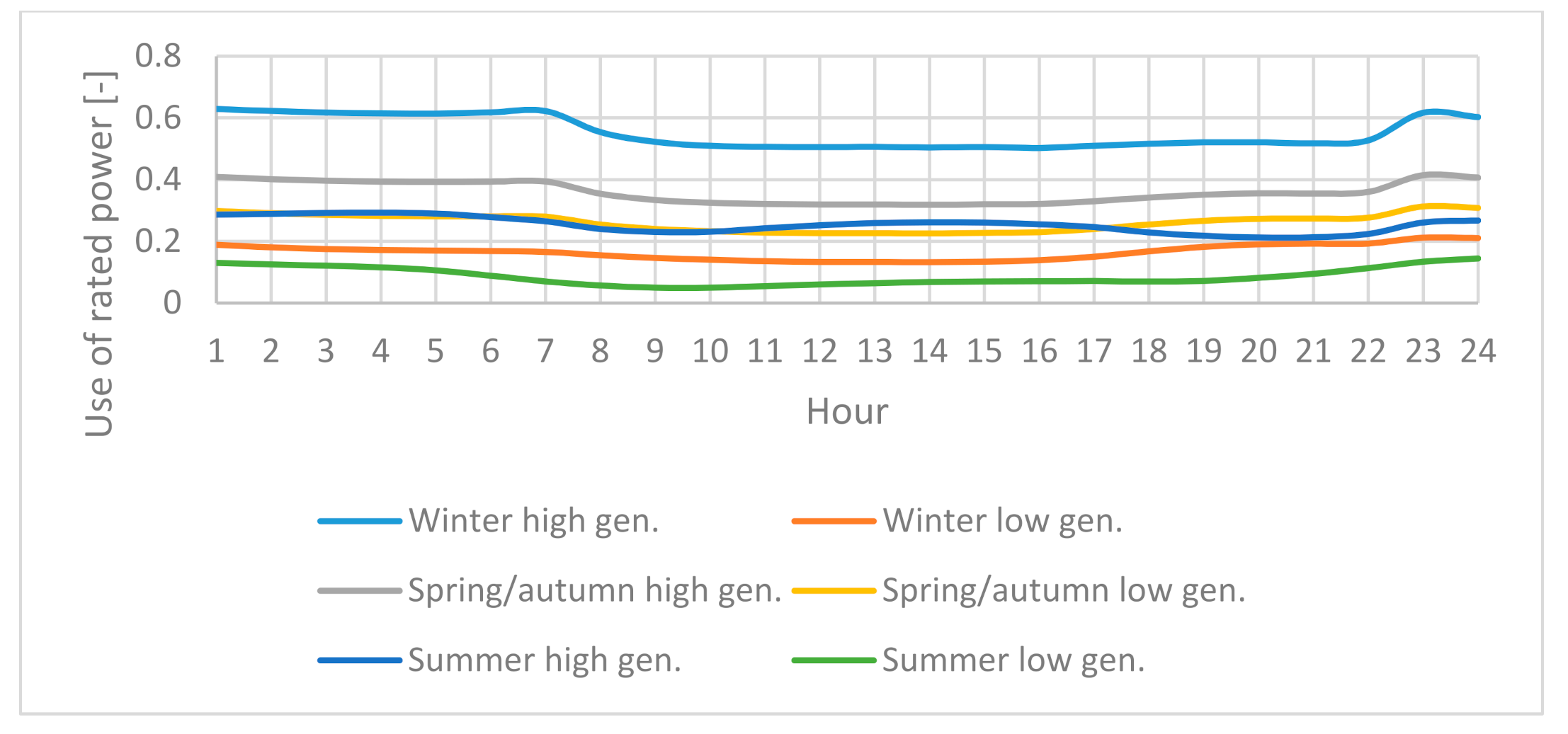
| generation profile for RES technology d in time t | |
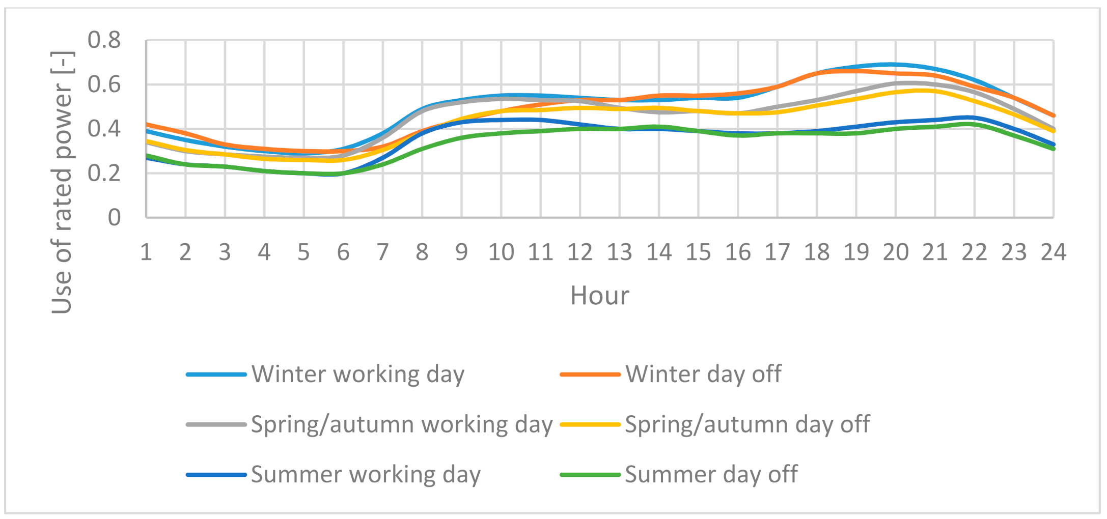
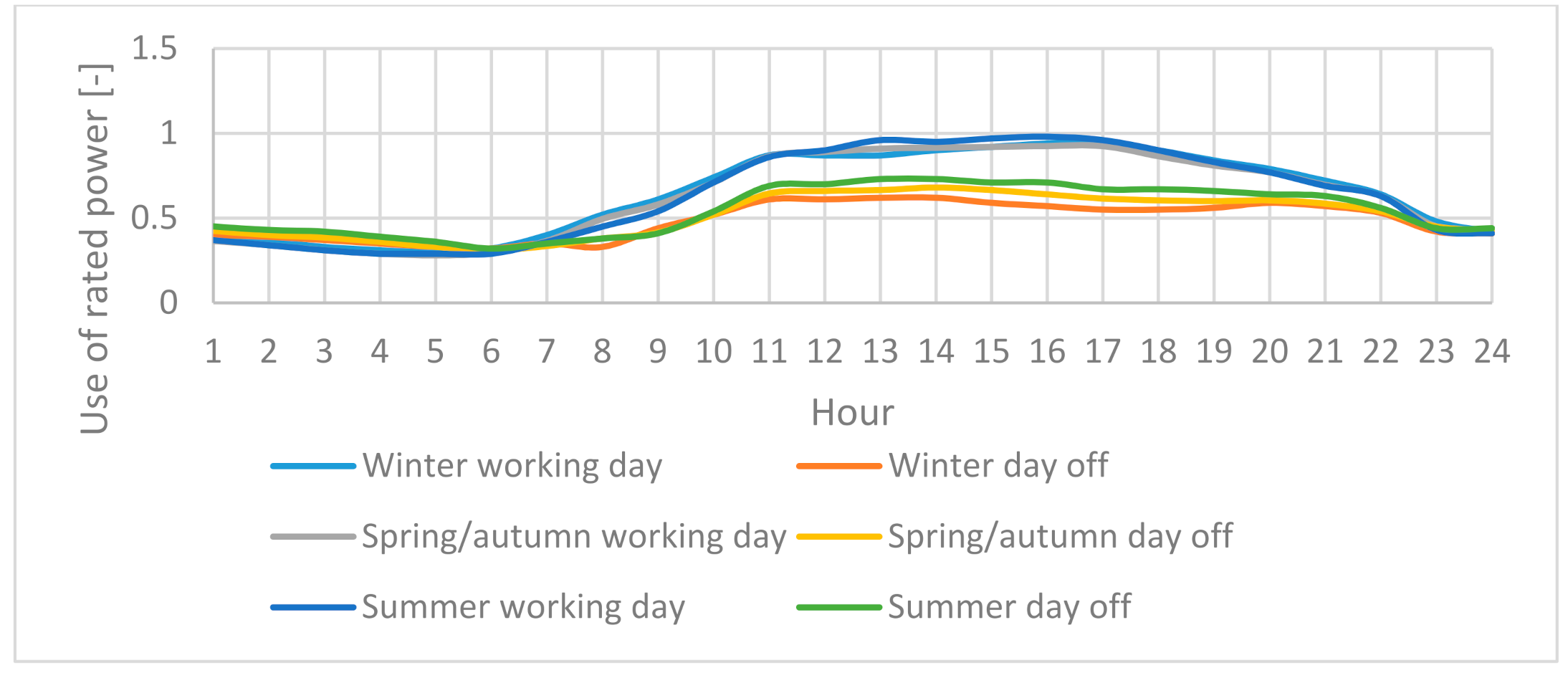
| consumption profile for load type l in time t | |
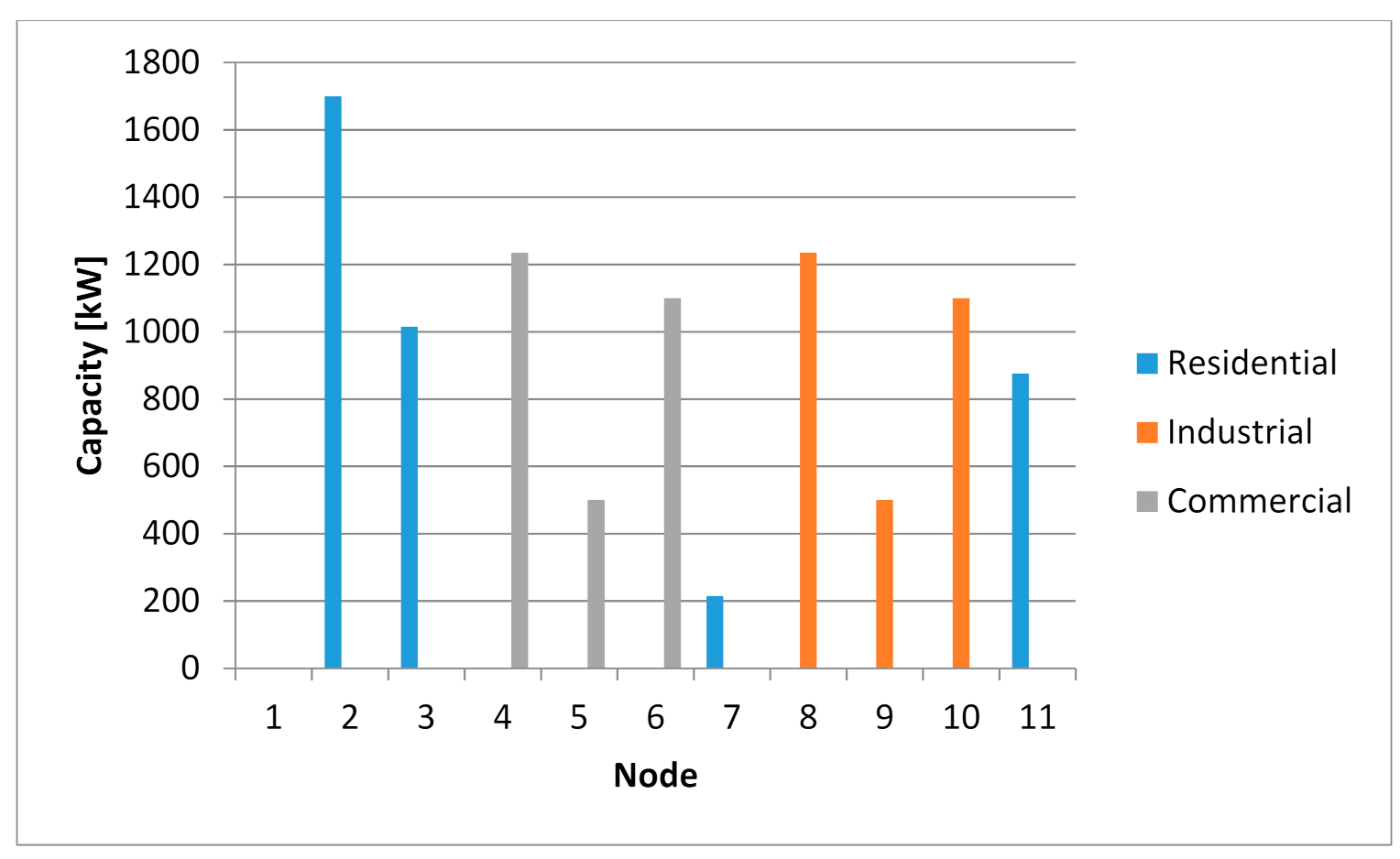
| nominal power of load type l in node n | |
| consumption of load in node n of type l in time t | |
| linearized power flow between nodes n and w in time t | |
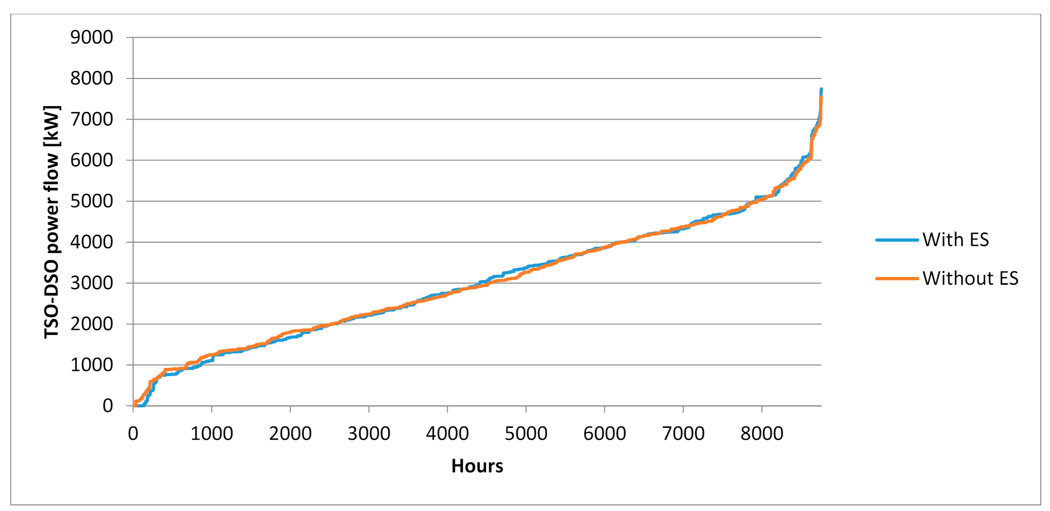
| energy exchange between distribution and transmission system in time t | |
| resistance of power line between nodes n and w | |
| nominal voltage of the distribution system (in this paper assumed as a 30 kV) | |
| value of voltage in nodes n/w in time t | |
| fixed cost of each type and rated power of renewable energy sources | |
| fixed cost of energy storages of type e | |
| fixed cost of new lines | |
| variable cost of each type d and rated power r of renewable energy sources | |
| level of charge of energy storages type e in node n in time t | |
| efficiency of energy exchange between nodes and energy storages | |
| Decision variable | |
| number of units in node n for RES type d and rated power r | |
| number of units in node n for energy storages for type e | |
| binary variable that determines whether a given “s” line will arise between the “n” and “w” nodes | |
| power which flow from grid to energy storage in node n in time t | |
| power which flow from energy storage to grid in node n in time t | |
| Acronyms | |
| wind turbine | |
| photovoltaic installation | |
| biogas power plant | |
| renewable energy sources | |
| ES | energy storages |
| GD | grid development |
Appendix A


References
- Mucha-Kuś, K.; Sołtysik, M.; Zamasz, K.; Szczepańska-Woszczyna, K. Coopetitive Nature of Energy Communities—The Energy Transition Context. Energies 2021, 14, 931. [Google Scholar] [CrossRef]
- Abu-Mouti, F.; El-Hawary, M. Optimal Distributed Generation Allocation and Sizing in Distribution Systems via Artificial Bee Colony Algorithm. IEEE Trans. Power Deliv. 2011, 26, 2090–2101. [Google Scholar] [CrossRef]
- Prenc, R.; Škrlec, D.; Komen, V. Distributed generation allocation based on average daily load and power production curves. Int. J. Electr. Power Energy Syst. 2013, 53, 612–622. [Google Scholar] [CrossRef]
- Kansal, S.; Sai, B.; Tyagi, B.; Kumar, V. Optimal placement of distributed generation in distribution networks. Int. J. Eng. Sci. Technol. 2011, 3, 47–55. [Google Scholar] [CrossRef]
- Keane, A.; O’Malley, M. Optimal utilization of distribution networks for energy harvesting. IEEE Trans. Power Syst. 2007, 22, 467–475. [Google Scholar] [CrossRef]
- Khalesi, N.; Rezaei, N.; Haghifam, M. DG allocation with application of dynamic programming for loss reduction and reliability improvement. Electr. Power Energy Syst. 2011, 33, 288–295. [Google Scholar] [CrossRef]
- Kuri, B.; Redfern, M.; Li, F. Optimization of rating and positioning of dispersed generation with minimum network disruption. In Proceedings of the IEEE Power Engineering Society General Meeting, Denver, CO, USA, 6–10 June 2004. [Google Scholar]
- Mashayekh, S.; Stadler, M.; Cardoso, G.; Heleno, M. A mixed integer linear programming approach for optimal DER portfolio, sizing, and placement in multi-energy microgrids. Appl. Energy 2017, 187, 154–168. [Google Scholar] [CrossRef] [Green Version]
- Carpinelli, G.; Mottola, F. Optimal allocation of dispersed generators, capacitors and distributed energy storage systems in distribution networks. In Proceedings of the 2010 Modern Electric Power Systems, Wroclaw, Poland, 20–22 September 2010; pp. 1–6. [Google Scholar]
- Garcia, R.; Weisser, D. A wind–diesel system with hydrogen storage: Joint optimisation of design and dispatch. Renew. Energy 2006, 31, 2296–2320. [Google Scholar] [CrossRef]
- Kahrobaee, S.; Asgarpoor, S.; Qiao, W. Optimum sizing of distributed generation and storage capacity in smart households. IEEE Trans. Smart Grid 2013, 4, 1791–1801. [Google Scholar] [CrossRef] [Green Version]
- Malaczek, M.; Wasiak, I.; Mienski, R. Improving quality of supply in small-scale low-voltage active networks by providing islanded operation capability. IET Renew. Power Gener. 2019, 13, 2665–2672. [Google Scholar] [CrossRef]
- Siczek, K.; Piersa, P.; Adrian, Ł.; Szufa, S.; Obraniak, A.; Kubiak, P.; Zakrzewicz, W.; Bogusławski, G. The Comparative Study on the Li-S and Li-ion Batteries Cooperating with the Photovoltaic Array. Energies 2020, 13, 5109. [Google Scholar] [CrossRef]
- Paiva, P.; Khodr, H.; Domínguez-Navarro, J.; Yusta, J.; Urdaneta, A. Integral planning of primary–secondary distribution systems using mixed integerlinear programming. IEEE Trans. Power Syst. 2005, 20, 1134–1143. [Google Scholar] [CrossRef]
- Türkay, B.; Artac, T. Optimal distribution network design using genetic algorithms. Electr. Power Compon. Syst. 2005, 33, 513–524. [Google Scholar] [CrossRef]
- Martins, V.; Borges, C. Active distribution network integrated planningincorporating distributed generation and load response uncertainties. IEEE Trans. Power Syst. 2011, 26, 2164–2172. [Google Scholar] [CrossRef]
- Vai, V.; Suk, S.; Lorm, R.; Chhlonh, C.; Eng, S.; Bun, L. Optimal Reconfiguration in Distribution Systems with Distributed Generations Based on Modified Sequential Switch Opening and Exchange. Appl. Sci. 2021, 11, 2146. [Google Scholar] [CrossRef]
- Jasiński, J.; Kozakiewicz, M.; Sołtysik, M. Determinants of Energy Cooperatives’ Development in Rural Areas—Evidence from Poland. Energies 2021, 14, 319. [Google Scholar] [CrossRef]
- Szablicki, M.; Rzepka, R.; Sołtysik, M.; Czapaj, R. The idea of non-restricted use of LV networks by electricity consumers, producers, and prosumers. In Proceedings of the 14th International Scientific Conference “Forecasting in Electric Power Engineering (PE 2018)”, Podlesice, Poland, 26–28 September 2018. [Google Scholar] [CrossRef]
- Wróbel, J.; Sołtysik, M.; Rogus, R. Selected elements of the Neighborly Exchange of Energy—Proftability evaluation of the functional model. Polityka Energ. Energy Policy J. 2019, 22, 53–64. [Google Scholar] [CrossRef]
- Andrychowicz, M. Comparison of the Use of Energy Storages and Energy Curtailment as an Addition to the Allocation of Renewable Energy in the Distribution System in Order to Minimize Development Costs. Energies 2020, 13, 3746. [Google Scholar] [CrossRef]
- Andrychowicz, M. RES and ES Integration in Combination with Distribution Grid Development Using MILP. Energies 2021, 14, 383. [Google Scholar] [CrossRef]
- PGE Dystrybucja S.A. Polish DSO. Available online: https://pgedystrybucja.pl/content/download/2038/file/iriesd_pge-dystrybucja-sa_tekst-jednolity_od_27_08_2020.pdf (accessed on 1 December 2020).
- Impact Assesment-Ocena Skutków Regulacji Do Projektu Ustawy o Odnawialnych Źródłach Energii. 12 November 2013. Available online: http://www.toe.pl/pl/wybrane-dokumenty/rok-2013?download=72:ocena-skutkow-regulacji (accessed on 1 December 2020).
- IRENA. Renewable Power Generation Costs in 2019. Available online: https://www.irena.org/-/media/Files/IRENA/Agency/Publication/2020/Jun/IRENA_Power_Generation_Costs_2019.pdf (accessed on 1 December 2020).
- NREL. 2019 Costs of Wind Energy Review. 2019. Available online: https://www.nrel.gov/docs/fy21osti/78471.pdf (accessed on 1 December 2020).
- PSE S.A. Polish TSO. Available online: https://www.pse.pl/dane-systemowe (accessed on 1 December 2020).
- 50HZ. Genrma TSO. Available online: https://www.50hertz.com (accessed on 1 December 2020).
- Amprion. German TSO. 2015. Available online: https://www.amprion.net/ (accessed on 1 December 2020).
- TeeneT. German TSO. Available online: http://www.tennet.eu/ (accessed on 1 December 2020).
- TransnetBW. German TSO. 2015. Available online: https://www.transnetbw.com (accessed on 1 December 2020).
- Nahmmacher, P.; Schmid, E.; Hirth, L.; Knops, B. Carpe diem: A novel approach to select representative days for long- term power system modeling. Energy 2016, 112, 430–442. [Google Scholar] [CrossRef]
- Lazard. Lazard’s Levelized Cost of Storage Analysis. November 2018. Available online: https://www.lazard.com/media/450774/lazards-levelized-cost-of-storage-version-40-vfinal.pdf (accessed on 1 January 2021).
- Andrychowicz, M. Optimization of distribution systems by using RES allocation and grid development. In Proceedings of the 15th International Conference of European Energy Market, Łodź, Poland, 27–29 June 2018. [Google Scholar]


| Technology | Capacity [kW] | ||
|---|---|---|---|
| Photovoltaic panels | 5 (Residential) | 50 (Commercial) | 500 (Industrial) |
| Wind turbines | 20 (Residential) | 100 (Commercial) | 1000 (Industrial) |
| Biogas power plants | 200 | 500 | 1000 |
| Technology | PV | WT | BG | ||||||
|---|---|---|---|---|---|---|---|---|---|
| Rated power [kW] | 5 | 50 | 500 | 20 | 50 | 500 | 200 | 500 | 1000 |
| Capital costs (overnight) [mln EUR/MW] | 1.37 | 0.94 | 0.75 | 4.37 | 3.58 | 1.2 | 3.06 | 2.85 | 2.7 |
| Fixed operating costs [thou. EUR/MW/annum] | 7.6 | 7.6 | 15.2 | 29.2 | 29.2 | 35.8 | 154.4 | 195.6 | 195.6 |
| Variable costs [EUR/MWh] | 0 | 0 | 0 | 0 | 0 | 0 | 87.3 | 74.7 | 66.9 |
| Type of ES | Capital Costs [EUR/kWh] | Fixed Operating Costs [EUR/kWh] |
|---|---|---|
| Residential | 580 | 69.5 |
| Industrial | 440 | 63.7 |
| Scenarios Group | Level of Energy from RES in Total Energy Consumption | |||||||
|---|---|---|---|---|---|---|---|---|
| ALL | 30% | 40% | 50% | 60% | 70% | 80% | 90% | 100% |
| ALL + ES | 30% | 40% | 50% | 60% | 70% | 80% | 90% | 100% |
Publisher’s Note: MDPI stays neutral with regard to jurisdictional claims in published maps and institutional affiliations. |
© 2021 by the author. Licensee MDPI, Basel, Switzerland. This article is an open access article distributed under the terms and conditions of the Creative Commons Attribution (CC BY) license (https://creativecommons.org/licenses/by/4.0/).
Share and Cite
Andrychowicz, M. The Impact of Energy Storage along with the Allocation of RES on the Reduction of Energy Costs Using MILP. Energies 2021, 14, 3783. https://doi.org/10.3390/en14133783
Andrychowicz M. The Impact of Energy Storage along with the Allocation of RES on the Reduction of Energy Costs Using MILP. Energies. 2021; 14(13):3783. https://doi.org/10.3390/en14133783
Chicago/Turabian StyleAndrychowicz, Mateusz. 2021. "The Impact of Energy Storage along with the Allocation of RES on the Reduction of Energy Costs Using MILP" Energies 14, no. 13: 3783. https://doi.org/10.3390/en14133783
APA StyleAndrychowicz, M. (2021). The Impact of Energy Storage along with the Allocation of RES on the Reduction of Energy Costs Using MILP. Energies, 14(13), 3783. https://doi.org/10.3390/en14133783