Optimal Transmission Line Switching to Improve the Reliability of the Power System Considering AC Power Flows

Abstract

The reliability of the electrical system is a fundamental study that is carried out to determine the possible deficiencies that an electrical system can have in case of failures, since a failure can cause disturbances, power cuts, and load disconnections. For this reason, Optimal Transmission Switching (OTS) with Optimal AC Power Flows (OPF-AC) is used to reduce disturbances when faults occur and minimize equipment load and disconnections, but OTS offers possible switches in order to make it possible to reduce the damage that can be done for a fault with operating limitations in voltage, power, and angular deviation. However, to have a complete study, it is proposed to use a reliability analysis through contingency ranking to know the risks that a switched system may have at the time of simultaneous or consecutive failures. In addition, a load capacity investigation is conducted to determine if the transmission lines are within their operating limits. The study presents an analysis of the behavior of the switched system and an adequate operation for the mitigation of failures in the system through the switching of transmission lines with analysis of load capacity and reliability. The results presented by the proposed methodology will be compared with Matlab’s Matpower simulation package.

1. Introduction

The electrical power system (EPS) distributes the electrical energy throughout the entire system so that the demand or final consumers can use it. For this reason, the generation system supplies the energy that needs to be distributed, the transmission system provides all the energy to the different energy consumption points that are normally required to operate, and the distribution system carries out the energy [1].

Each of the systems that make up the EPS are configured so that they can support the demand, and this study is carried out by planning both the generation system and the transmission system that are expanded in accordance with the growth in population consumption. This is why expansion and planning studies are carried out in order to maintain the service and control of the system. By knowing the development of the demand, it is possible to plan the expansion of the system; one method is the planning through the Optimal Switching of Transmission Lines (OTS), which allows for carrying out expansion studies and is exposed by [2,3,4].

EPS can also become vulnerable when system failures occur, such as short circuit failures, lightning strikes, electrical disturbances, connection, and disconnection of large electrical charges, etc. Electrical failures produce variations in the voltage operation, angle, in frequency and mainly in the electrical energy balance (generated power must be the same as the power required by the final consumer) [5,6,7]; when the fault is not appropriately solved, it can lead to a complete disconnection of the system. A reliability study allows for knowing which devices are vulnerable against failures and verifies the behavior of the EPS; for this reason, an N-1, N-2 reliability analysis is performed to determine the reliability of the EPS [8].

The N-1 contingency means that there will be a disconnection of one element in the system, such as a transmission line, generator, transformer, etc.; meanwhile, N-2 is the disconnection of two devices. Reliability indexes are used for a reliability study in order to quantify which equipment is more susceptible to failures. These indexes can be applied to power generation, transmission, or distribution [9]. There is another way to quantify which devices are more susceptible to affect the system in case of failures; this method is known as contingency ranking, and it can be calculated by the power flow of the transmission lines. When a contingency ranking is performed, if the value obtained is minimal, it means that its value is close to zero. The probability of failure is reduced, but, if the ranking value is high, the probability of damage by a failure is high [10].

Using OTS, it can be guaranteed that there is no disconnection of the electrical demand. The important thing about OTS is to minimize the impact on the system due to a disconnected line, but, when there is a disconnection of the lines, there is an increase in the power flow, and this increase can saturate or overcharge them. Therefore, when there is a switching, this inconvenience must be solved and the functionality of the EPS must be safeguarded [11].

In order to maintain EPS functionality, OST uses voltage, angle, frequency, and power balance as the parameters for line disconnection; in case a variable is outside of operating limits, it is checked and scanned for other elements to be switched. OST is used to solve various EPS problems, such as expansion analysis investigated by [2,3]; troubleshooting disconnection problems; and modifying power flow to maintain operability, reduce, or minimize electrical faults proposed by [12,13,14].

The most important thing is to provide electric power through the transmission system and the disconnection of end consumers could be carried out as little as possible. It is important that OST changes the topology of the electrical network to keep the system operational in case of instability, but, at the time of switching, it might be able to modify the voltage levels in the system, and it will make changes in the power flow of the transmission lines, but the main thing is to mitigate the faults. This means eliminating them from the electrical system [5,7,15]; in summary, OST optimizes power generation [16], restructures the system, redesigns the topology, changes the power flow to continue normal supply to end consumers, and maintains the operation of the EPS [17].

Therefore, it is proposed to use OST to minimize the variations of the electrical parameters when a fault occurs in the EPS, and, by the usage of OST, the fault is mitigated, the electrical fault is isolated, and, by means of the disconnection of the transmission lines, the EPS topology is altered. This can affect the power flow, voltages, and angles [12,18]. The objective is to characterize the electrical system through the switching of the transmission lines and to verify which are the vulnerable transmission lines in the new topology produced by the OTS. By means of a loadability analysis and a contingency ranking, the vulnerability can be determined. Through the OPF-AC, the normal state of the system will be known, and it will be possible to compare it with the scenarios after different N-3 contingencies. The presented results of the methodology will be compared with the Matpower simulation package in Matlab by means of the average error.

This article is organized as follows: Section 2 presents optimal switching of transmission lines. Section 3 provides the reliability, Section 4 problem formulation, and Section 5, results obtained. Finally, Section 6 presents the conclusions.

2. Optimal Transmission Switching

OST is a method that allows for maintaining the power distribution, but the system reliability may vary because the operating parameters change and are mainly due to the switching of the lines. The system is restructured and mainly the reliability decreases because the system is operating without the connection of several elements of the system. In addition, it also produces an increase in power flow and the system stability point changes, but these are necessary measures to be taken in case of a system failure that may cause disconnections of distribution systems and losses of final consumers [19,20]. OST allows for solving several problems that may occur in the system, several authors have presented the mathematical model of OTS, and there are several theorems that were presented after the implementation and verification for each of the models presented by [13]. In addition, several authors perform OST by means of OPF-DC [8,21] and others for getting a better accuracy of the model use OPF-AC [21,22].

The big difference between OPF-DC and OPF-AC is that OPF-DC is a faster convergence optimization; that is, it uses fewer resources in the optimization and the type of problem is mixed integer linear programming MILP with binary variables. On the other hand, OPF-AC has a wider convergence time, it uses more programming resources, and the type of problem is mixed integer nonlinear programming MILNP with binary variables [18,23,24]. The binary variables represent those transmission lines that are enabled for the transfer of electric power, verifying the behavior of the system before and after a disturbance or fault. It is so important to know the state of the system and the switching of the transmission lines before and after the fault [25,26]; by means of switching, it is possible to maintain the power supply. In addition, the OST restructures the topology of the system, it changes the path of the power flow, and it minimizes the operating cost due to the presence of electrical disturbances [19,20].

The key point of using the OTS is to keep the system stable, isolate electrical faults, and satisfy the electrical energy balance [27,28]. When a switching is performed, there are parameters that are affected, such as voltage level, frequency, angular deviation, and electrical losses. For this reason, an analysis of the behavior of the parameters must be performed, and it must be verified that each parameter is operating under normal conditions and under operating criteria. This means that it does not exceed the established ranges of operation by performing analysis through optimal power flows, the operating status of the system before and after the disturbance can be checked, and an adequate switching can be established, with the purpose of maintaining a constant flow of energy and an adequate operation of the basic parameters in which the system can work.

Objective Function:

$$Z=\sum _i(c{b}_i\ast Pge{n}_i)$$

(1)

Dependent to OPF AC restrictions:

$$P_{ij}=V_i\ast V_j\ast [B_{ij}\ast sin({\theta }_i-{\theta }_j)]$$

(2)

$$Q_{ij}=V_i^2\ast B_{ij}-V_i\ast V_j\ast [B_{ij}\ast cos({\theta }_i-{\theta }_j)]$$

(3)

$$\sum _{ij}\left(Pge{n}_i\right)-\sum _i\left(P{d}_i\right)=\sum _{ij}\left(P_{ij}\right)$$

(4)

$$\sum _{ij}\left(Qge{n}_i\right)-\sum _i\left(Q{d}_i\right)=\sum _{ij}\left(Q_{ij}\right)$$

(5)

Equation (1) is the target function, which proposes the minimization of the total cost times the production of the generated power “Z”. This is in reference for the multiplication of the cost produce of each plant cb times the power that is going to generate each plant “Pgen”.

Equations (2) and (3) are the power flow equations and flow through the transmission lines both in active and reactive power; these equations are in function of voltage, angle, and susceptance.

Equations (4) and (5) are the power balance equations; this means that the power generated minus the power required by the demand, it must be equal to the flow existing in the transmission lines. The power balance must be fulfilled both for the active power Equation (4) and for the reactive power Equation (5)

$$P_{ij}-V_i\ast V_j\ast B_{ij}\ast sin({\theta }_i-{\theta }_j)\le (1-{\psi }_{ij})\ast ML$$

(6)

$$P_{ij}-V_i\ast V_j\ast B_{ij}\ast sin({\theta }_i-{\theta }_j)\ge ({\psi }_{ij}-1)\ast ML$$

(7)

$$Q_{ij}+V_i\ast V_j\ast B_{ij}\ast cos({\theta }_i-{\theta }_j)\le (1-{\psi }_{ij})\ast ML$$

(8)

$$Q_{ij}+V_i\ast V_j\ast B_{ij}\ast cos({\theta }_i-{\theta }_j)\ge ({\psi }_{ij}-1)\ast ML$$

(9)

Equations (6)–(9) are the power flow equations but with the OST comparison. $\psi$ represents the binary variable and ML represents the OST constant. Equations (6) and (7) are the active power flow of the line, through $(1-{\psi }_{ij})$, which it must be verified that the line is not switched, and, if it is switched, the power flow will take a value of zero; Equations (8) and (9) are the reactive power flow comparing with the variable that it represents if the line is switched. Thus, the state of the transmission line will be verified:

$$\sum _{ij}(1-{\psi }_{ij})\le NSL$$

(10)

$$B_{ij}=1/X_{ij}$$

(11)

$${\psi }_{ij}\in 0,1$$

(12)

$$P_{ij}=\sum _j\left(P_{ij}\right)\ast {\phi }_i$$

(13)

Equation (10) refers to the comparison that the sum of switched lines $\psi$ must be less than or equal to the number of lines allowed by the NSL algorithm; this restriction allows for quantifying how many switched lines are permitted for each electrical system. Equation (11) refers to the calculation of the susceptance, through the reactance of the transmission line. Equation (12) is the initialization of the binary variable and represents the state of the transmission lines, 0 switched and 1 line connected. Equation (13) is the verification of the flow of the lines when there is switching:

Restrictions of the OTS and OPF-AC:

$$P_{ij}^{min}\ast {\psi }_{ij}\le P_{ij}\le P_{ij}^{max}\ast {\psi }_{ij}$$

(14)

$$Q_{ij}^{min}\ast {\psi }_{ij}\le Q_{ij}\le Q_{ij}^{max}\ast {\psi }_{ij}$$

(15)

Equations (14) and (15) refer to the comparison of the active power and reactive power with the upper and lower limits, but these limits are multiplied by the binary variable that shows if the line is switched; if it is switched, its comparison will be with zero, both in its lower and upper limits.

Equations (16) and (17) refer to the comparison of the power of each generator, with its lower limits and upper limits, both in the active power Equation (16) and in the reactive power equation:

$$Pge{n}_{ij}^{min}\le Pge{n}_{ij}\le Pge{n}_{ij}^{max}$$

(16)

$$Qge{n}_{ij}^{min}\le Qge{n}_{ij}\le Qge{n}_{ij}^{max}$$

(17)

These are the levels allowed for the electrical system to be under voltage operability criteria when there is a charge increase or a disconnection or failure in the EPS. Several authors mention that there is an instability voltage and a collapse voltage that depends on the charge increase; when a system is at the voltage collapse levels, the system automatically produces a blackout or general blackout of the EPS, a method to perform a voltage stability study is by analyzing the PV curve. By means of the PV curve, the stable voltage points, critical instability points, and voltage collapse point can be determined [29,30,31]. According to several studies and research, the voltage operating limits or voltage stability limits are 10% of the nominal operating value [31]. It gives both minimum and maximum values in which the system can operate; and this we can observe in Equation (18)

$$V_i^{min}\le V_i\le V_i^{max}$$

(18)

These are the variations that can occur when a fault is generated in the EPS. There are two types of instability, transient and oscillatory instability, the time in which the instability occurs is a short duration; and the angular deviation is produced by angular instability or loss of synchronism of the electrical generators. By means of the power curve vs. angle, it allows for knowing the limits of angular stability allowed [29,32]. Through the Equation (19), the maximum and minimum limits of angular operation allowed in the EPS are established:

$${\theta }_i^{min}\le {\theta }_i\le {\theta }_i^{max}$$

(19)

When the loadability of transmission lines is mentioned, it refers to the power that a transmission line can transfer from the generation system to the final consumer. When a system is operating under normal conditions, the lines have a power flow that is represented by the charge of the line, but, when there is a change in the flow after a disturbance in the system or failure, this charge increases or decreases [33,34]. There are several methods that limit the power flow, in order not to charge the lines and maintain the power supply; by means of the OST the system is restructured, the fault is isolated, and mainly it is intended to maintain the operating parameters of the system and maintain the power balance of the electrical system. The mathematical formulation for the calculation of the charge ability of the transmission lines is presented:

$$C{a}_{ij}=\frac{P_{ij}}{SI{L}_{ij}}$$

(20)

Equation (20) is the calculation of the line charge, where it is presented through the division between the power transmitted by the line P${}_{ij}$ and the maximum power allowed by the transmission line $SIL$${}_{ij}$.

3. Reliability

Reliability is a process that lets us know the security or confidence that exists in the electrical system. The fundamentals of Reliability, a verification of the system, are to know the vulnerable equipment when a disturbance or failure occurs, and what are the minimum operating requirements that the EPS can support [35]. Reliability contributes to knowing what level of contingency can support the system, and which elements of the system are vulnerable; but a contingency refers to an element that goes out of operation either by failure or by bad maneuvers of the equipment. This means that the equipment is not available and, through some studies, a solution must be provided on how to maintain stability and provide electrical service in unusual conditions [2,8,24].

A reliability study of the EPS allows for knowing the system behavior, and it has to be done in normal operation and in a failure state. However, a system can have a great variety of devices such as lines, transformers, and substations that may fail; therefore, it is common to perform an analysis of those elements that have a higher probability on not operating or those that do not possess redundancy [35,36]. To know the EPS behavior when an element of the system normally stops working due to the presence of an electrical failure is the focus of one study N-1 [21,37]. It is well-known that when an electrical failure occurs and only one element of the system is affected, the system has the capacity to maintain its operation because of the stagnation of the electrical generators [9,22].

To perform a reliability analysis, reliability indices or contingency rankings are used to find out which elements are most likely to cause instability [38,39,40]. The methodology uses the contingency ranking to know the status of each transmission line and verify how the lines behave when there is commutation in the EPS; the mathematical formulation of the contingency ranking can be seen in the following Equation (21).

$$R{a}_{ij}=\frac{{\left(P_{ij}\right)}^2}{2\ast {\left(SI{L}_{ij}\right)}^2}$$

(21)

The contingency ranking calculation allows for knowing which line has less reliability in the system. Equation (21) is expressed by the power division, which transmits the line and the maximum power of the transmission line.

4. Problem Formulation

The case study of the Ecuadorian 230 kV transmission system is presented in Figure 1. In the

Table 1. Demand data.

Demand	Pd	Qd	Demand	Pd	Qd
Demand 1	21.7	12.7	Demand 15	8.2	2.5
Demand 2	14	1.2	Demand 16	7	1.8
Demand 3	0	0	Demand 17	18	5.8
Demand 4	25	1.6	Demand 18	0	0
Demand 5	94.2	19	Demand 19	3.2	0.9
Demand 6	22	10.9	Demand 20	9.5	3.4
Demand 7	30	30	Demand 21	10	0.7
Demand 8	0	0	Demand 23	0	0
Demand 10	15	2	Demand 24	0	0
Demand 11	0	0	Demand 26	0	0
Demand 12	11.2	7.5	Demand 29	10	2.3
Demand 14	0	0	Demand 09	5.8	2
Demand 13	6.2	1.6	Demand 25	17.5	11.2
Demand 27	10	1.6	Demand 28	15	6.7

,  

Table 2. Transmission line data.

Line	${\mathit{R}}_{\mathit{ij}}$	${\mathit{X}}_{\mathit{ij}}$	SIL	Line	${\mathit{R}}_{\mathit{ij}}$	${\mathit{X}}_{\mathit{ij}}$	SIL
L1–2	0.02	0.0575	130	L 14–25	0.0727	0.1499	32
L1–5	0.05	0.1852	130	L15–16	0.0116	0.22	32
L2–5	0.06	0.1737	65	L15–17	0.1	0.202	16
L3–4	0.01	0.0379	130	L15–18	0.115	0.18	16
L4–10	0.05	0.02	130	L16–17	0.132	0.27	16
L4–11	0.06	0.1763	65	L17–21	0.1885	0.3292	16
L4–5	0.01	0.0414	90	L17–22	0.2544	0.38	16
L5–6	0.05	0.116	70	L17–28	0.1093	0.2087	16
L6–26	0.03	0.082	130	L17–29	0.2198	0.4153	16
L6–27	0.01	0.09	32	L18–19	0.3202	0.6027	16
L6–7	0.13	0.255	32	L19–20	0.2399	0.453	16
L6–8	0.06	0.130	32	L19–22	0.0636	0.2	32
L7–18	0.09	0.120	32	L22–23	0.0169	0.06	32
L7–8	0.221	0.12	16	L23–24	0.0639	0.1292	16
L7–9	0.08	0.193	16	L28–29	0.034	0.068	32
L10–11	0.107	0.218	16	L14–17	0.0348	0.0749	32
L11–12	0.063	0.129	16	L13–15	0.0324	0.0845	32
L11–13	0.034	0.068	32	L13–14	0.0936	0.2.9	32

and  

Table 3. Generation data.

Generator	Cost	Pmin	Pmax	Qmin	Qmax
Gen 3	2	0	120	0	150
Gen 4	1.75	0	120	−20	60
Gen 7	1	0	100	−15	44.7
Gen 8	3.25	0	110	−15	62.5
Gen 9	3	0	60	−10	40
Gen 10	3	0	80	−15	48.7
Gen 13	1	0	250	0	250
Gen 14	1.75	0	120	−20	60
Gen 15	1	0	100	−15	44.7
Gen 20	3.25	0	110	−15	62.5
Gen 22	3	0	60	−10	40
Gen 23	3	0	80	−15	48.7
Gen 24	2	0	120	0	150
Gen 25	1.75	0	120	−20	60
Gen 26	1	0	100	−15	44.7
Gen 27	3.25	0	110	−15	62.5
Gen 28	3	0	60	−10	40
Gen 29	3	0	80	−15	48.7

that will be displayed the electrical demand data, transmission lines data and generators data respectively, data that are required for the proposal algorithm.

Figure 1 shows the georeferencing of the Ecuadorian electrical system, where, in the figure, the busbar, the demand, and the transmission lines can be seen. The diagram represents the national 230 kV interconnected system. It can be seen in the figure that there is redundancy in the system, which helps to improve its reliability to keep the electrical service stable.

4.1. Study Case

The objective is to characterize the behavior of the system when forming the commutation of the transmission lines up to an N-3 contingency. Thus, it is intended to know if the system can withstand an N-3 contingency and verify if it is possible to maintain the operation of the system, under the operating criteria, such as that the system is within the voltage margins, in the angular deviation margins in which the transmission lines are not overloaded due to the change of flow due to the switching of the lines, and through a contingency analysis that verifies the vulnerable lines of the system.

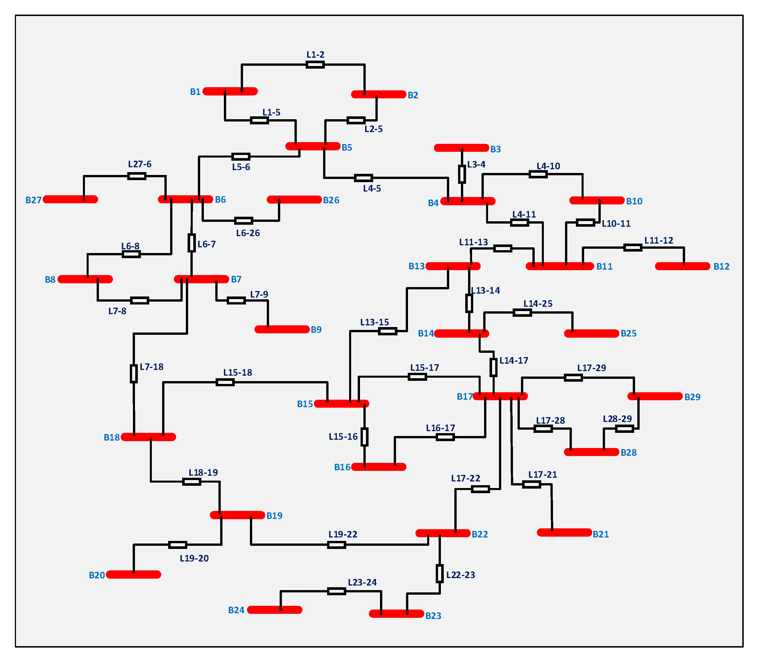
Figure 2 represents the electrical circuit of the system that is under analysis, but only with the impedances of the system; that is, the impedances of the transmission lines and the status of their connection. The system found as a case study has 29 bars and these can be viewed in Figure 2. The data presented in Table 1,  Table 2 and  Table 3 are the starting parameters for the proposed methodology.

Table 1 is the demand power of each system connection busbar; that means, it is the power that the generators must supply; the active power “Pd” and reactive power “Pq” are found in [MW] and [MVAR].

Table 1 presents the data of the transmission lines, which are used to calculate the algorithm, and the table values presented are: resistance “$R_{ij}$” in [pu], reactance “$X_{ij}$” in [pu], and the maximum power that each transmission line can transmit “SIL” (surge impedance loading) in [MW].

Table 3 is all the necessary data of the generator, the maximum and minimum active power “Pmax and Pmin” in [MW], the maximum and minimum reactive power “Qmin and Qmax” in [MVAR], and the operating cost of each generator in “[$/MW]”.

4.2. Methodology

The proposed methodology is used to verify the behavior of the system in a normal operating state, and when there are three switched transmission lines, that is, with an N-3 contingency. It is verified that the normal operation and contingency scenarios N-3 are within the voltage and angular deviation margins. In addition to the scenarios, a loadability analysis and contingency analysis are carried out—in order to establish if the case study has the capacity to operate under contingencies (N-3) and under what conditions the system will operate in or be during a critical point of operation. Everything mentioned can be seen in the algorithm. The algorithm presented is a compilation of the methods presented by the authors [13,14]. However, the methodology presented by the authors is in DC and what is proposed is to carry out a study in AC that includes an analysis of chargeability and ranking of contingencies; to do this, all the expressions found in Equations (1)–(21) are used, and these equations are included in the proposed algorithm.

Algorithm 1 OST with loadability analysis and contingency rankings

Step: 1 Input data Powers, Reactances, Resistances and operating costs. Generators: $Pge{n}^{max}$, $Pge{n}^{min}$, $Qge{n}^{max}$, $Qge{n}^{min}$, cb Transmission línes: R, X, SIL Electrical demand: Pd, Pq Step: 2 Impedance and admittance calculations $B=1÷X$ $Zbus=\sqrt{(}{R}^2+X^2)$ $Ybus=1÷\sqrt{(}{R}^2+X^2)$ $thbus=arctan(X÷R)$ Step: 3 OPF–AC O.F.:  Min $Z={\sum }_i(c{b}_i\ast Pge{n}_i)$ s.t.:  $P_{ij}=V_i\ast V_j\ast [B_{ij}\ast sin({\theta }_i-{\theta }_j)]$  $Q_{ij}=V_i^2\ast B_{ij}-V_i\ast V_j\ast [B_{ij}\ast cos({\theta }_i-{\theta }_j)]$  ${\sum }_{ij}\left(Pge{n}_i\right)-{\sum }_i\left(P{d}_i\right)={\sum }_{ij}\left(P_{ij}\right)$  ${\sum }_{ij}\left(Qge{n}_i\right)-{\sum }_i\left(Q{d}_i\right)={\sum }_{ij}\left(Q_{ij}\right)$ Step: 4 OTS – based on OPF–AC F.O.:  Min $Z={\sum }_i(c{b}_i\ast Pge{n}_i)$ s.t.:  $P_{ij}-V_i\ast V_j\ast B_{ij}\ast sin({\theta }_i-{\theta }_j)\le (1-{\psi }_{ij})\ast ML$  $P_{ij}-V_i\ast V_j\ast B_{ij}\ast sin({\theta }_i-{\theta }_j)\ge ({\psi }_{ij}-1)\ast ML$  $Q_{ij}+V_i\ast V_j\ast B_{ij}\ast cos({\theta }_i-{\theta }_j)\le (1-{\psi }_{ij})\ast ML$  $Q_{ij}+V_i\ast V_j\ast B_{ij}\ast cos({\theta }_i-{\theta }_j)\ge ({\psi }_{ij}-1)\ast ML$  ${\sum }_{ij}(1-{\psi }_{ij})\le NSL$  ${\psi }_{ij}\in 0,1$  $P_{ij}={\sum }_j\left(P_{ij}\right)\ast {\phi }_i$ Step: 5 Loadability analysis $C{a}_{ij}=\frac{P_{ij}}{SI{L}_{ij}}$ Step: 6 Contingency ranking $R{a}_{ij}=\frac{{\left(P_{ij}\right)}^2}{2\ast {\left(SI{L}_{ij}\right)}^2}$

The presentation Algorithm 1 is exposed in six steps. The first step comments on all the data necessary to run the algorithm. The second step provides the calculation of the impedances and admittances. In the third step, the calculation of the optimal power flow in AC is carried out. Through the OPF-AC, the following will be known: the powers supplied by each generator, the power flow of each line, the voltage level, and the angular deviation of each bus. In the fourth step, the contingency N-3 will be calculated and thus it will be determined which are the possible disconnections in such a way that they do not drastically affect the system at the level of voltage and angular deviation. In the fifth step, the loadability analysis is calculated for each of the scenarios. Finally, a contingency analysis is conducted for each scenario in the sixth step.

5. Results

The results of the methodology proposed in Section 4 are presented in the following section. These results are the behavior of the system in a normal operating state and for an N-3 contingency; that is, a maximum number of three switched lines. These scenarios will be compared to verify the changes presented. For them, the behavior of the system is verified in the following parameters: voltage, angular deviation, power flow, loadability of the transmission lines, and, finally, the contingency analysis for each scenario is presented. In addition, the results obtained from the methodology will be compared through a simulation package such as Matpower, and this package is programmed in Matlab. The verification is carried out by calculating the average error between the Matpower simulation package vs. the results of the proposed algorithm.

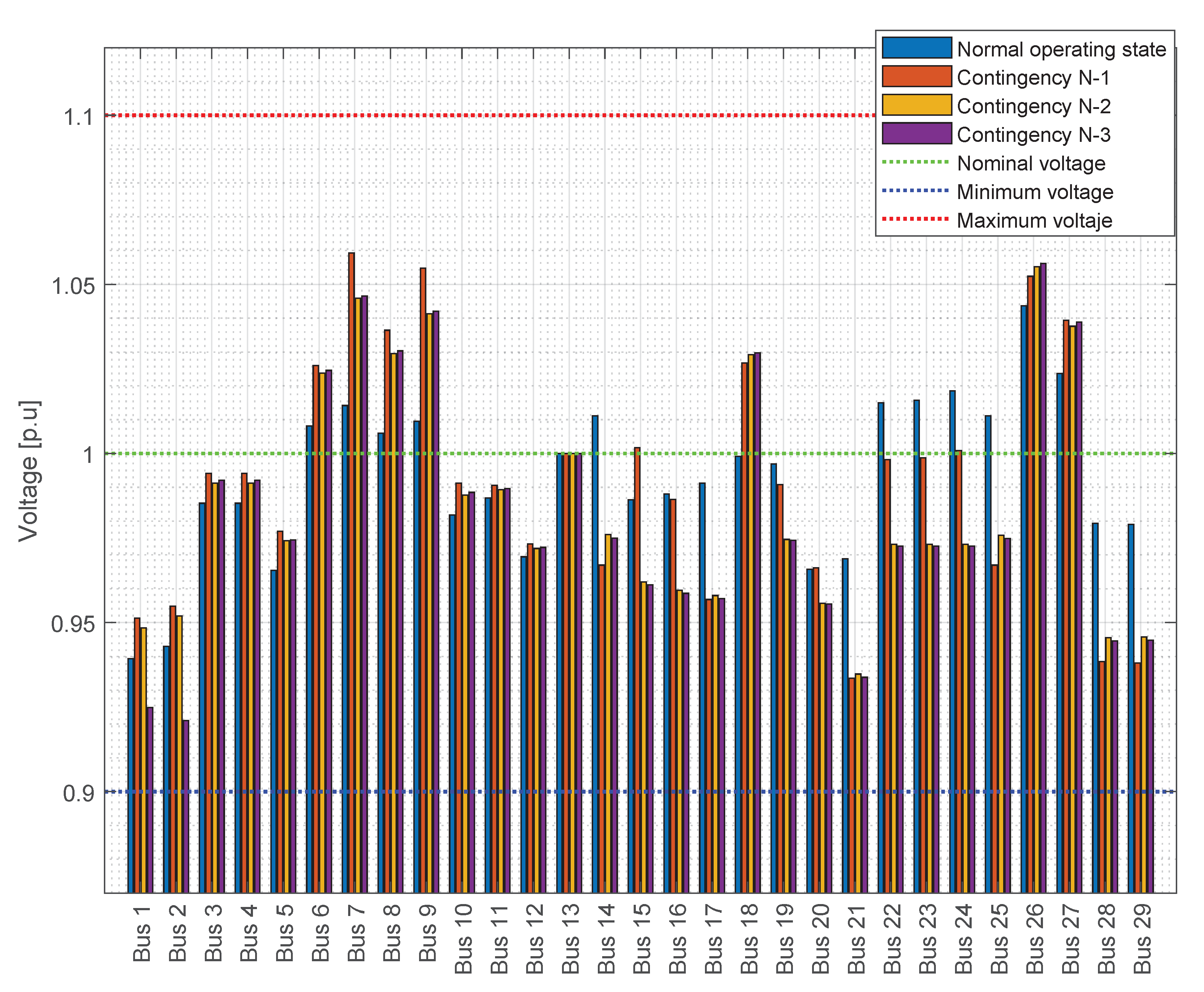
Figure 3 shows the voltage variations that occur in each scenario, in the main scenario which is the normal operation of the system vs. each of the contingencies that arise. The figure shows how the voltage varies for each switched line. An important point is that the voltage levels are within the 10% voltage stability margins, and these margins are highlighted in the figure. In addition, in many bars, the reduction of the voltage level can be verified. For example, in bars 14, 15, 16, and 17, there is a reduction of the voltage level. This is due to the switched transmission lines since the switched transmission lines are connected in these bars. These changes in the voltage level of the busbars reduce reliability and, with each change in the voltage level, the behavior of each of the elements that are connected in the electrical system will also be affected.

Figure 4 shows the behavior of the power flow that circulates through the transmission lines, and it is seen how the power flow varies when switching occurs. In the lines that are not close to the generation bars, there is a minimal change in the behavior of the power flow—for example, for lines 17–28, 6–27, 10–11, and 11–12, the power flow is very similar in each study scenario.

You can also verify in Figure 4 the switched lines in each scenario. In the N-1 contingency scenario (one switching line), the transmission line is 15–17. For the contingency scenario N-2, the switched lines are 13–15 and 15–18. In the contingency scenario N-3, the switched lines are 13–15, 15–18, and 2–5. All of these switching lines caused changes in the power flow, which decreases the reliability of the system.

Another important aspect in Figure 4 is that, for the transmission lines that are connected to the generation busbars, there is a greater change in the power flow. This is because the power flow increases or decreases to maintain the operation of the system. For example, lines 1–5, 2–5, 7–18, and 16–17 have variations in power flow due to the switches presented.

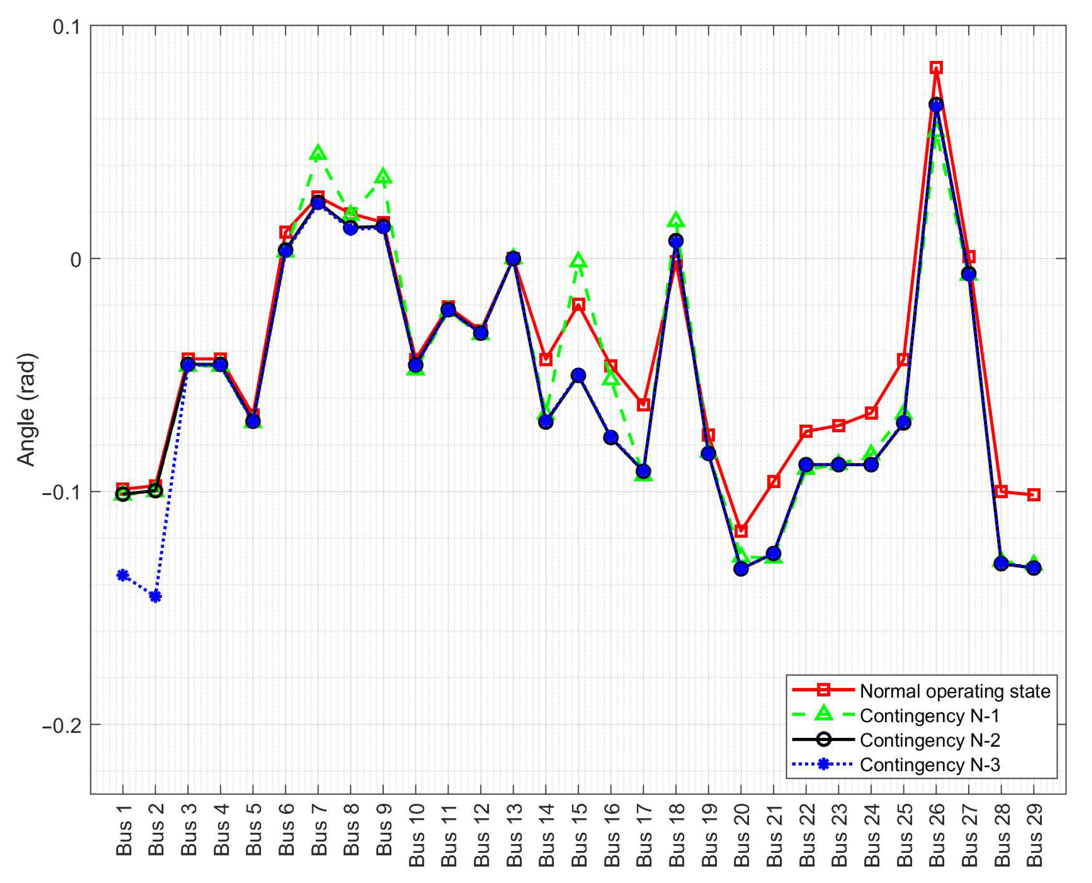
Figure 5 shows the behavior of the angular variation that occurs in each scenario, for the contingencies caused and in the normal operating state of the system. In Figure 5, it can be seen that the angular variation during the three switching has a moderate variation. It also reflects that, for the busbars where generators and neighboring busbars are present, they have a great presence of angle changes; for example, busbar 4, busbar 5, busbar 10, busbar 12, and busbar 13.

Another important aspect that can be verified in Figure 5 is the behavior of all the busbars. Such behavior is that none of the busbars operate outside the established limits, or that they are in a point that is closer to the upper or lower limit of 0.52 radians ($\pi$/6); this means that the system in terms of angular variation does not present any inconvenience and it can normally operate.

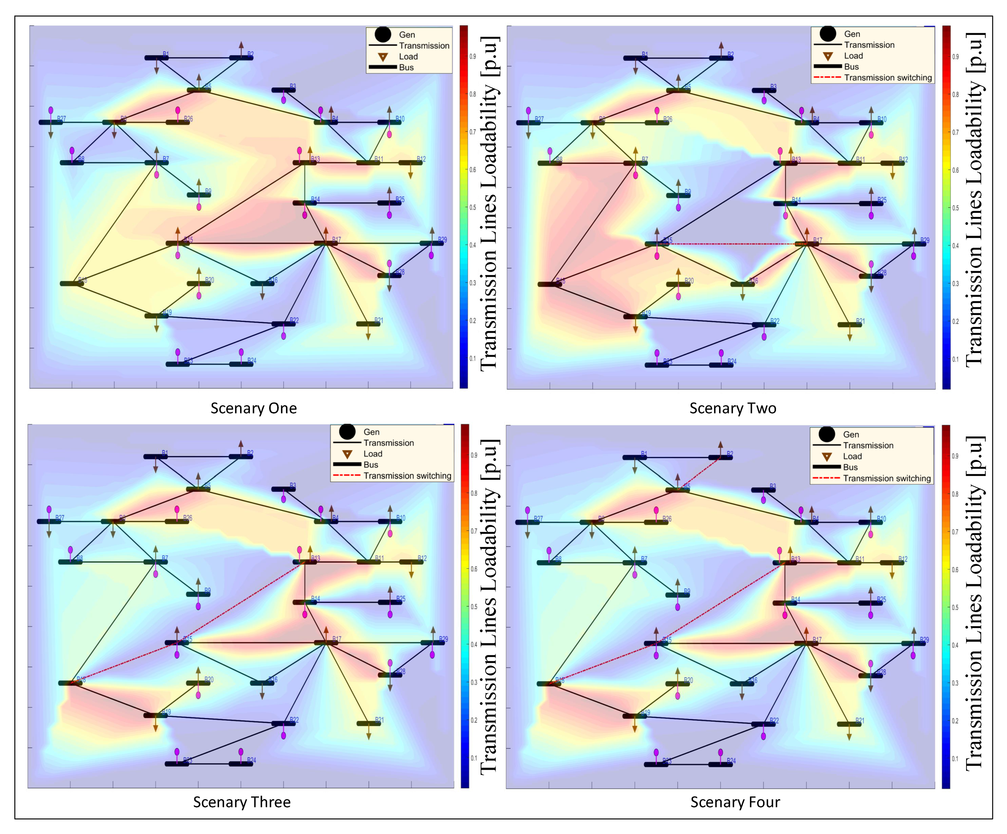
Figure 6 shows the system behavior in terms of loadability of the transmission lines, which was done by using color trends. The system behavior can be seen, where the lines that are connected only to the demand have a minimum variation, but, in contrast to those lines that are close to the generators, there is an increase or change in their charge level, due to the commutations carried out.

In Figure 6, the loadability of the system in each of the scenarios can be seen. The first scenario is when you are operating under normal conditions. Scenario 2 is when it is subjected to a contingency, Scenario 3 in two contingencies and Scenario 4 with three contingencies. In the first scenario, a figure is presented with an overload in several transmission lines. In Scenario 2, switching lines 15–17 shows a drastic change in several lines that were not overloaded, and this produces a change in the power flow. In Scenario 3 with switching lines 15–18 and 13–15, it can be seen that the performance of the transmission system is very similar to Scenario 1, and it is not as drastic as in Scenario 2. For Scenario 4 with switching lines 15–18, 13–15, and 2–5, as well as Scenario 3, the variation of the power flow is similar, and there is an increase in the power flow, but it is not as drastic as in Scenario 2. An important point of the system is its redundancy, since, in Scenario 2, lines 15–17 are disconnected, which has a load of 1 [p.u], but the system has the ability to redirect the power flow.

Table 4. Contingency ranking for transmission lines.

Contingency	L17–28	L15–17	L14–17	L11–13	L5–6	L18–19	L13–14	L16–17	L7–18
None	0.5	0.5	0.5	0.48	0.46	0.19	0.11	0.03	0.21
N-1	0.5	switched	0.5	0.48	0.46	0.49	0.5	0.5	0.44
N-2	0.5	0.5	0.46	0.48	0.46	0.5	0.5	0.04	0.12
N-3	0.5	0.5	0.46	0.48	0.46	0.5	0.5	0.04	0.13

provides the contingency ranking of each of the scenarios of the case study proposed, and you can see the behavior of several lines. In the first scenario where the system operates normally, there are transmission lines that have a contingency of 0.5 and, for the study system, it is a considerable contingency. Of the three contingencies presented, it can be seen that the one with the highest incidence is Scenario 1, since the disconnection is directly from the loaded line, as can be seen in Figure 6. However, also through the analysis, it is corroborated that this causes lines 18–19, 13–14, 16–17, and 7–18 to be more vulnerable in the system, in the event of a disconnection or failure.

Table 5. Comparative analysis between average error in [p.u] of Algorithm vs. MatPower.

	Without Switching	1 Switching	2 Switching	3 Switching
Generator Active Power	0.02	$0.01$	0.06	0.06
Generator Reactive Power	0.15	0.19	0.09	0.1
Nodal Voltage	0.009	0.005	0.005	0.005
Power of the lines	0.0905	0.0994	0.0915	0.131
Nodal angle	0.144	0.215	0.1952	0.208

contains the comparison between the proposed methodology and the simulation of the system in the Matpower simulation package that is embedded in Matlab. The values obtained are per unit. The results in the table are the average error values of each of the indices described in the system. It can be verified that the error is minimal among the results obtained. On the other hand, the behavior of the generators has an estimated value of 0.02 p.u. Otherwise, the nodal tension presents the estimated error of 0.009 p.u. These values are similar. They are also variations and have similar responses. The system has the same behavior regarding the flow of the line, the voltages of each node, and the behavior of the generators. Therefore, it is important to mention that the results are similar, and the proposed methodology provides similar responses to the simulation package.

6. Conclusions

The methodology presented is a great tool that allows for a complete study of the transmission system, mainly checking if the system has the capacity to withstand contingencies and how it would behave in case of failures. In the study presented for an N-1 contingency, it can be said that the commutation is of a fully loaded line and the system was able to maintain its operation, but this caused several lines to be overloaded to mitigate the commutation and causes the system to be vulnerable if a new failure occurs.

It can also be said that the methodology presented is a reliable tool because the results obtained are very similar to the results presented by the simulation package. In addition to complying with the voltage and angle operating margins, these parameters are important to maintain the operation of the system in suitable conditions for the end users.

The proposed methodology is only used to perform system analysis when transmission lines are disconnected, but the system is operating in its entirety and is not operating in island mode. This means that, when a failure occurs and, in order to maintain its operation, the system needs to be divided into two or three electrical systems, the proposed methodology cannot present results of its behavior or its vulnerabilities.

7. Future Work

In the future, there is a plan to develop new research which will be confirmed in collaboration with stability analyses and verify if the system is outside the inflection points of a disconnection or experiences total failure of the power electrical system.