Short-Term Load Forecasting Using Neural Networks with Pattern Similarity-Based Error Weights

Abstract

Forecasting time series with multiple seasonal cycles such as short-term load forecasting is a challenging problem due to the complicated relationship between input and output data. In this work, we use a pattern representation of the time series to simplify this relationship. A neural network trained on patterns is an easier task to solve. Thus, its architecture does not have to be either complex and deep or equipped with mechanisms to deal with various time-series components. To improve the learning performance, we propose weighting individual errors of training samples in the loss function. The error weights correspond to the similarity between the training pattern and the test query pattern. This approach makes the learning process more sensitive to the neighborhood of the test pattern. This means that more distant patterns have less impact on the learned function around the test pattern and lead to improved forecasting accuracy. The proposed framework is useful for a wide range of complex time-series forecasting problems. Its performance is illustrated in several short-term load-forecasting empirical studies in this work. In most cases, error weighting leads to a significant improvement in accuracy.

1. Introduction

Time series (TS) often exhibit complex seasonal patterns. For example, hourly data may have a daily periodicity, a weekly periodicity, and a yearly periodicity. Sometimes, it also exhibits a monthly periodicity. Typical examples of this type of TS can be found in the energy sector: energy consumption TS, electricity load TS, wind and solar power production TS, and electricity prices TS in wholesale markets. Accurate forecasts of the load, energy production, and electricity prices are essential for power system planning, control, and scheduling and for energy markets. In this study, our focus is on short-term load forecasting (STLF), which uses hourly, half-hourly, or quarterly TS with daily, weekly, and yearly seasonalities. Figure 1 shows periodograms of such TS for four European countries, which we use in the experimental part of this work. As can be see from this figure, the daily seasonality dominates significantly over the other ones for PL, GB, and DE data. For FR data, the yearly seasonality is much stronger than others. Note that 12 h seasonality is also revealed and is related to the characteristic shape of the daily profile (see the lower panel of Figure 2). This seasonality is even stronger than the weekly one for PL and FR data. Due to multiple seasonality, nonlinear trend, daily shape changing significantly during the week and during the year, and random fluctuations, the STLF problem is challenging and requires the forecasting model to be highly flexible.

In addition to the energy sector, the demand variations in the transportation, telecommunications, tourist, and healthcare sectors can also be greatly influenced by multiple seasonal cycles [1,2,3,4]. In order to deal with TS expressing multiple seasonality, the forecasting model should be equipped with appropriate mechanisms. Over the years, many methods of performing this have been proposed.

1.1. Forecasting Models for TS with Multiple Seasonality

A standard autoregressive moving average (ARMA) model for single seasonality can be extended to multiple seasonal cycles [5]. In the double seasonal formulation, two new terms need to be introduced to the ARMA model. These terms are polynomial functions, involving backshifts of the seasonal period. Similarly, to include a third seasonal cycle, two new terms need to be introduced. ARMA models for triple seasonality contain 21 adjustable parameters. A drawback of the seasonal ARMA model is the assumption that the cycle shapes are all the same. In practice, the seasonal patterns can greatly differ from each other. For example, in STLF, daily cycles for workdays can be significantly different from those for weekends.

Another popular and widely used statistical forecasting procedure, the Holt–Winters method, which belongs to the class of exponential smoothing methods (ETS), was extended to incorporate a second seasonal component in [6] and a third seasonal component in [7]. The adaptation involves the inclusion of second and third seasonal indexes and two additional smoothing equations for these indexes. The triple seasonal Holt–Winters model is composed of five interdependent equations that express a smoothed level, three seasonal indexes, and an additive combination of them. It requires the selection of five smoothing parameters and initial values for the level and seasonal cycles. As with ARMA, the seasonal Holt–Winters model suffers from an important weakness. It requires the same cyclical behavior for each period. To incorporate distinct seasonal patterns into the model, first, they should be identified in some way and, then, the model formulation should be developed [7].

To deal with changing seasonal patterns, innovation state-space models for ETS were employed in [8]. They can forecast TS with either additive (linear) or multiplicative (nonlinear) seasonal patterns. Their fundamental goal for multiple seasonal processes is to allow for the seasonal terms that represent a seasonal cycle to be updated more than once during the period of the cycle. This goal may be achieved by dividing the basic cycle into several shorter subcycles and by updating the seasonal terms of one sub-cycle during the time for another subcycle. Thus, for each day of the week, a separate subcycle can be used. Having too many subcycles complicates the model and increases the number of parameters to adjust. To reduce complexity, Gould et al. [8] proposed introducing common seasonal patterns for different subcycles. The limitation of the model is that it can only be used for double seasonality, where one seasonal length is a multiple of the other.

An interesting extension of the innovation state-space modeling framework for forecasting complex seasonal TS, such as those with multiple seasonal periods, high-frequency seasonality, non-integer seasonality, and dual-calendar effects was proposed in [9]. It combines an ETS state space model with Fourier terms, a Box–Cox transformation, and ARMA error correction. The seasonal components in this framework are represented by trigonometric functions based on Fourier series. The Fourier trigonometric representation with time-varying coefficients enables both linear and nonlinear TS with non-integer seasonal frequencies to be modeled. The Box–Cox transformation helps to transform the data into normality and to handle nonlinearities.

Among the newer statistical models for forecasting TS with multiple seasonality, it is worth mentioning the Prophet [10]. This model is optimized for business forecasting tasks, which typically have any of the following characteristics: hourly, daily, or weekly observations; strong multiple “human-scale” seasonalities, such as day of week and time of year; important holidays that occur at irregular intervals; historical trend changes, for instance due to product launches or logging changes; and trends that are nonlinear growth curves, where a trend hits a natural limit or saturates. The Prophet procedure is an additive regression model with four main components: a piecewise linear or logistic growth curve trend, a yearly seasonal component modeled using Fourier series, a weekly seasonal component using dummy variables, and a user-provided list of important holidays. According to the authors, due to its flexible formulation, Prophet can easily accommodate seasonality with multiple periods.

Machine learning (ML) methods offer an alternative to classical statistical forecasting methods. They provide forecasting models with the ability to learn about historical patterns and anomalies and to improve prediction accuracy. Among the ML methods, neural networks (NN) are most often used for forecasting. There are numerous forecasting model solutions based on different NN architectures [11]. The way to deal with multiple seasonality varies depending on the base model, the mechanisms used, and the authors’ creativity. For example, the winning submission to the most reputable forecasting competition, M4 Makridakis, in a version for hourly double seasonal TS combines ETS to deal with seasonality and recurrent NN [12]. An ETS module, in the form of a double seasonal Holt–Winters model, produces two seasonal components. These are used for TS deseasonalization and adaptive normalization during on-the-fly preprocessing. The preprocessed TS is forecasted by a long short-term memory (LSTM) network that is composed of two blocks of two dilated LSTM layers. A dilation mechanism allows for the LSTM cells to take into account the earlier hidden states, which in this case, are shifted back in time by 1, 4, 24, and 168 h. This improves long-term memory performance and can be especially useful for seasonal TS, as it expresses a cyclical relationship between the series elements.

Another LSTM-based model (LSTM-MSNet) for TS with multiple seasonal patterns was proposed recently in [13]. It is a globally trained LSTM network, where a single prediction model is built across all of the available TS to exploit the cross-series knowledge. According to the authors, this enables the model to untap the common seasonality structures and behaviors available in a collection of TS. To deal with multiple seasonal cycles, LSTM-MSNet initially uses a deseasonalization strategy to detach the multiseasonal components from a TS. For deseasonalization, different statistical decomposition techniques were utilized including Fourier transformation. LSTM was trained on the seasonally adjusted TS or, in the second variant, on the original TS together with the seasonal components as exogenous variables. The choice of the learning variant was determined by the characteristics of the TS.

Although recurrent NNs, such as LSTM, gated recurrent units, and DeepAR [14], dominate today as NN architectures applied to TS forecasting, other solutions for multiple seasonal TS are also used. For example, in [15], a deep NN architecture based on backward and forward residual links and a very deep stack of fully connected layers was proposed. In this model, each stack is composed of basic building blocks. In the generic architecture, each block learns the predictive decomposition of the partial forecast in the basis matrix. This matrix expresses waveforms in the time domain, which composes, together with the learnable expansion coefficients, the partial forecast. In the interpretable architecture, each block can model a trend or a seasonal component. In the latter case, the basis function has the form of Fourier series with learnable Fourier coefficients. Thus, the partial forecast produced by each block is a periodic function mimicking typical seasonal patterns. The final forecast is the sum of partial forecasts produced by all the blocks. Thus, complex seasonal pattern can be decomposed and modeled by many blocks. Another deep architectures useful for forecasting multiple seasonal TS was proposed in [16]. It extends the canonical transformer architecture [17] by introducing a convolutional self-attention mechanism, which allows the model to better incorporate the local context of the TS. An experimental study performed on the TS exhibiting both hourly and daily seasonal patterns showed that the proposed approach achieved state-of-the-art performance in comparison with recent RNN-based methods.

The approaches presented above for multiple seasonal TS forecasting rely on incorporation into the model mechanisms, which allow it to deal with seasonal components. An alternative approach is to simplify the problem by TS decomposition. The components expressing less complexity than the original TS can be modeled independently using simpler models. The most popular methods of decomposition are additive decomposition, multiplicative decomposition, seasonal-trend decomposition using LOESS, discrete Fourier and wavelet transforms, and empirical mode decomposition [18,19,20,21].

Another method of dealing with TS with multiple seasonal periods was proposed for STLF in [22] and described further in the context of neural models in [23]. This pattern-based approach uses TS representation expressing the shapes of basic seasonal cycles. A trend and seasonal cycles longer than the basic cycle are filtered out from the TS. Thus, the relationship between TS elements is simplified and can be modeled using simple models such as nonparametric regression models based on similarity [24] or shallow NNs [25]. After forecasting the preprocessed TS, the trend and seasonal components are determined from the most recent TS history and combined with the forecasted seasonal pattern. It is worth emphasizing that this approach needs neither a complex forecasting model for multiple seasonal TS nor TS decomposition and forecasting of each component individually. Experimental research has confirmed that these models can compete in terms of accuracy with state-of-the-art deep learning models, such as the winning M4 submission [26].

1.2. Neural Networks for STLF

Due to their very attractive properties, useful for solving forecasting problems, NNs are widely used in STLF [27]. They are competitive with the state-of-the-art ML models such as support vector regression, random forest, and gradient boosting decision trees [28]. A survey of the classical NN architectures for STLF can be found in [29,30], and a comparison of their performances can be found in [25]. New NN architectures are quickly applied in STLF. Some examples are given below.

• A hybrid model based on a deep convolutional NN is introduced for short-term photovoltaic power forecasting in [31]. In this approach, different frequency components of the TS are first decomposed using variational mode decomposition, and then, they are constructed into a two-dimensional data, which can be better learned by convolution kernels, leading to a higher prediction accuracy.
• LSTM NN was proposed in [32] for STLF for individual residential households. Forecasting an electric load of a single energy user is fairly challenging due to the high volatility and uncertainty involved. LSTM can capture the subtle temporal consumption pattern persisting in single-meter load profile and can produce the accurate forecasts.
• Deep residual networks were proposed for STLF in [33]. The proposed model is able to integrate domain knowledge and researchers’ understanding of the task by virtue of different NN building blocks. Specifically, a modified deep residual network was formulated to improve the forecast results and a two-stage ensemble strategy was used to enhance the generalization capability of the proposed model. The model can be applied to probabilistic load forecasting using Monte Carlo dropout.
• Stacked denoising autoencoders were used in [34] for forecasting the hourly electricity price. The model was equipped with a unsupervised pre-training process to prevent overfitting. It incorporates concepts of the random sample consensus and stochastic neighbor embedding to further improve the forecasting performance.
• Pooling-based deep recurrent NN was applied in [35] for household load forecasting. A novel pooling-based deep learning was proposed, which batches a group of customers’ load profiles into a pool of inputs. The model aims to directly learn the uncertainty of load profiles by applying deep learning.
• A hybrid model based on randomized NN for probabilistic electricity load forecasting was proposed in [36]. This model includes generalized extreme learning machine for training an improved wavelet NN, wavelet preprocessing, and bootstrapping. It takes into account data noise uncertainties while the output of the model is the load probabilistic interval.
• Second-order gray NN using wavelet decomposition was proposed in [37] to improve the accuracy of load forecasting. In this approach, the load TS is decomposed by wavelet decomposition to reduce the nonstationary load sequence. Then, a second-order gray forecasting model is used to forecast each component of the TS. To obtain the optimal parameters, the NN mapping approach is used to build the second-order gray forecasting model.
• A wavelet echo state network was applied to both STLF and short-term temperature forecasting in [38]. A wavelet transform was used as the front stage for multi-resolution decomposition of the TS. Echo state networks function as forecasters for decomposed components. A modified shuffled frog leaping algorithm is used for optimizing the model.
• A spiking NN for STLF was proposed in [39]. This model employs spike train models that are close to their biological counterparts. An implementation of the proposed model is divided into two phases. In the first phase, spike NN predicts a day-ahead hourly temperature profile. In the second phase, another spike NN predicts a day-ahead load profile based on actual and forecasted temperatures, historical loads, day of the week, and holiday effect.
• Convolutional NNs are combined with fuzzy TS for STLF in [40]. In this approach, multivariate TS data, which include hourly load data, hourly temperature TS, and fuzzified version of load TS, were converted into multi-channel images to be fed to a proposed convolutional NN model.
• Deep residual network with a convolution structure was proposed to STLF in [41]. The authors analyzed and discussed the effectiveness of the convolutional residual network with different hyperparameters and architectures that include depths, widths, block structures, and shortcut connections, with/without dropout.
• Convolutional NNs combined with a data-augmentation technique, which can artificially enlarge the training data, were applied for STLF a single household in [42]. This method can address issues caused by a lack of historical data and improves the accuracy of residential load forecasting, which is a fairly challenging topic because of the high volatility and uncertainty of the electric demand of households.

1.3. Summary of Contributions

In this work, we propose an innovation to the pattern-based neural model for forecasting TS with multiple seasonality such as STLF. To improve the NN learning performance, we introduce error weights to the mean square error loss function. The weights assigned to the training patterns are dependent on the similarity between the training patterns and the query test pattern. This modification makes the learned mapping function more accurate in the neighborhood of the query test pattern and leads to improved forecasting performance.

The weighted loss function in NNs was used in many different formulations and contexts. In [43], to address the class distribution imbalance in deep learning, a class re-balancing strategy based on a class-balanced dynamically weighted loss function was proposed. In this approach, the weights are assigned based on class frequency and predicted probability of ground truth class. A similar problem, data imbalance problem, was considered in [44]. In this study, the weighted loss function has two types of weights, i.e., a class balanced weight and a sample importance weight. The sample importance weights discriminate between samples of different importance considering the sample difficulty (the performance of the classifier on the sample). A dynamically weighted loss function for convolutional and recurrent deep architectures was proposed in [45]. This approach is expected to modify the learning process by augmenting the loss function with a weight value corresponding to the learning error of each data instance. The objective is to force deep learning models to focus on those instances where larger learning errors occur in order to improve their performance.

In contrast to the approaches described above, our method proposed in this work assigns weights to the training patterns depending on their similarity to the query test pattern. The goal is to model the target function around the query pattern with greater accuracy.

The contribution of this study includes the following two points:

• We propose a new univariate multi-step forecasting neural model with pattern similarity-based error weighting for TS with multiple seasonality.
• We empirically demonstrate using challenging STLF problems the statistically significant accuracy improvement and forecasting bias reduction of the proposed approach with respect to the standard approach without error weighting.

The rest of the work is organized as follows. Section 2 describes the pattern representation of the TS. Section 3 presents the forecasting neural model with error weighting. The experimental framework used to evaluate the performance of the proposed approach is described in Section 4. Finally, Section 5 concludes the work.

Table 1. List of the main symbols.

Symbol	Meaning
${\left\{E_k\right\}}_{k=1}^K$	time series of length K
${\mathbf{e}}_i={[E_{i,1}{E}_{i,2}\dots E_{i,n}]}^T$	vector expressing a daily TS sequence of day i
${\overline{e}}_i$, ${\tilde{e}}_i$	mean value and dispersion of sequence ${\mathbf{e}}_i$, respectively
${\widehat{\mathbf{e}}}_{i+\tau }$	forecasted daily sequence
n	length of the daily sequence; length of the input and output patterns
N	number of training samples
m	number of hidden nodes
$r_i$, $r_i^{\prime }$	rank and normalized rank of i-th training sample, respectively
${\mathbf{x}}_i={[x_{i,1}{x}_{i,2}\dots x_{i,n}]}^T$	input pattern
${\mathbf{y}}_i={[y_{i,1}{y}_{i,2}\dots y_{i,n}]}^T$	output pattern
$\gamma$	parameter controlling the weighting function shape
$\tau \ge 1$	forecast horizon in days
$\Psi ={\left\{({\mathbf{x}}_i,{\mathbf{y}}_i)\right\}}_{i=1}^N$	training set
${\omega }_i$	error weight for ith training sample

lists the main symbols used in this study.

2. Multiple Seasonal Time Series and Their Representation

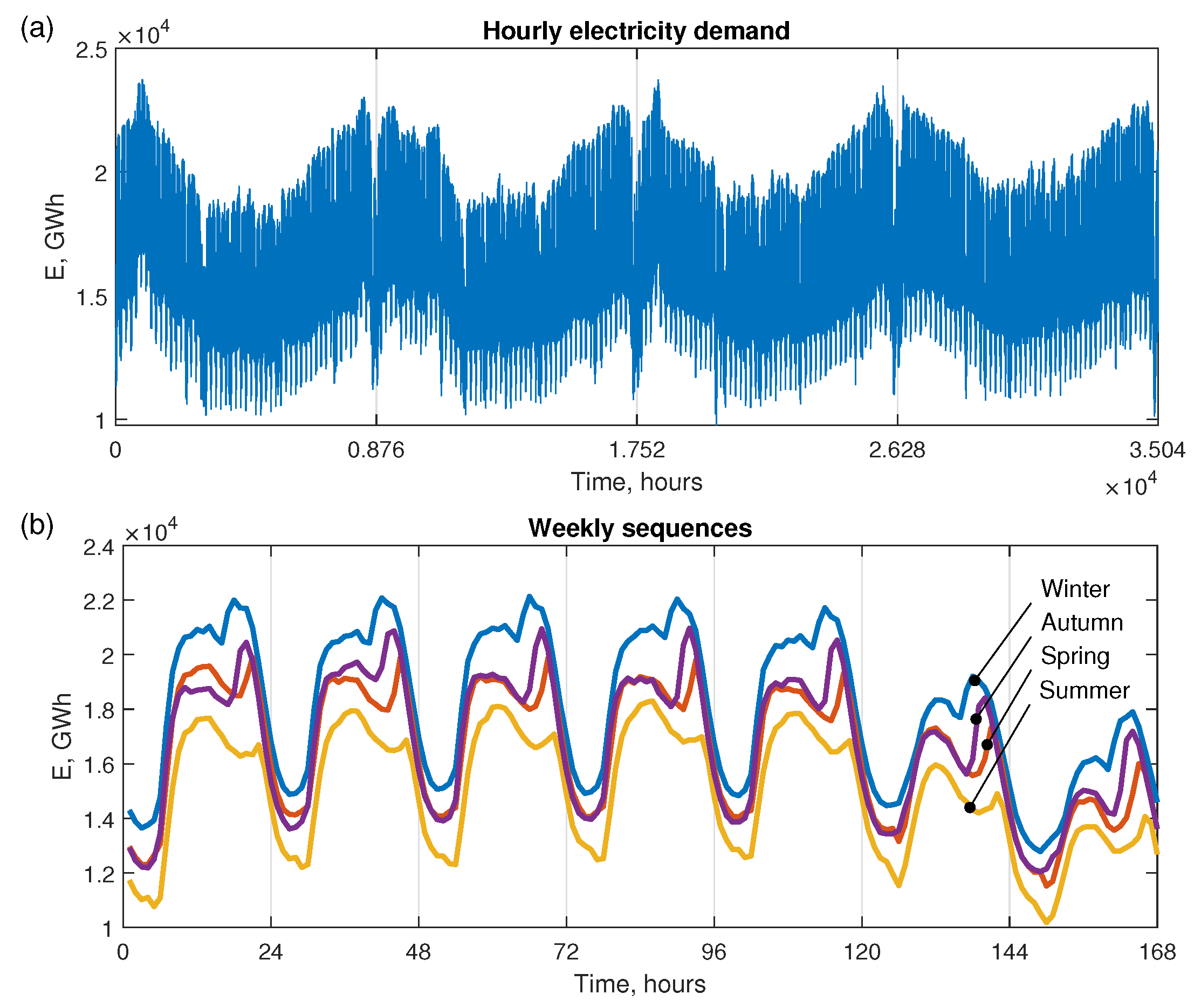
Let us consider the hourly electricity demand TS for Poland as an example of TS with multiple seasonality. This TS is shown in Figure 2 for the 4-year period 2012–2015. As can be seen from this figure, it exhibits a trend and three seasonal cycles: annual, weekly, and daily. Note that the daily shape changes significantly during the week and during the year.

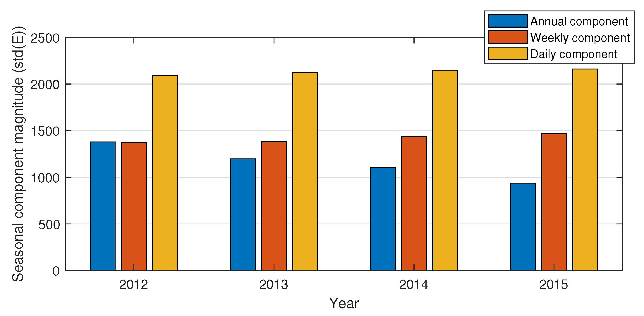
To estimate the magnitudes of the seasonal components, we calculate the standard deviations as follows. For annual seasonality, we calculate the weekly means and their standard deviations in each yearly period. For weekly seasonality, we calculate the daily means and their standard deviations in each weekly period. Finally, for daily seasonality, we calculate the standard deviations of hourly demand in each daily period. These standard deviations correspond to the magnitudes of the seasonal components. Their values, averaged over the yearly periods, are shown in Figure 3. For annual variations, we can observe a steady fall in the variability of the weekly mean demands over the years. The weekly and daily components rise slightly over the years. The strongest seasonal component in this TS is the daily one.

The TS representation used in this study produces input and output patterns. The input patterns represent predictors as transformed sequences of the daily period, while the output patterns represent the forecasted daily sequences. The transformations that turn the TS into patterns are aimed at normalizing daily sequences by unifying the variance and by removing the trend as well as longer seasonal cycles (weekly and annual cycles in our case). The resulting patterns express normalized shapes of the daily sequences.

Let ${\left\{E_k\right\}}_{k=1}^K$ be a TS and ${\mathbf{e}}_i={[E_{i,1}{E}_{i,2}\dots E_{i,n}]}^T$ be a vector expressing a daily TS sequence of day i. This sequence of length n (24 for the hourly TS) is represented by input pattern ${\mathbf{x}}_i={[x_{i,1}{x}_{i,2}\dots x_{i,n}]}^T$, which is determined as follows:

$${\mathbf{x}}_i=\frac{{\mathbf{e}}_i-{\overline{e}}_i}{{\tilde{e}}_i}$$

(1)

where ${\overline{e}}_i$ is a mean value of sequence ${\mathbf{e}}_i$ and ${\tilde{e}}_i=\sqrt{{\sum }_{t=1}^n{(E_{i,t}-{\overline{e}}_i)}^2}$ is a measure of sequence ${\mathbf{e}}_i$ dispersion.

The x-pattern defined by this equation is a normalized version of centered vector ${\mathbf{e}}_i$. Due to the pattern representation, the TS daily sequences, which have a different mean value and dispersion, are unified. All x-patterns, representing successive daily sequences, have zero mean, the same variance, and the same unity length. However, they differ in shape.

The output pattern ${\mathbf{y}}_i={[y_{i,1}{y}_{i,2}\dots y_{i,n}]}^T$ represents the forecasted daily sequence ${\mathbf{e}}_{i+\tau }={[E_{i+\tau ,1}{E}_{i+\tau ,2}\dots E_{i+\tau ,n}]}^T$, where $\tau \ge 1$ is a forecast horizon in days. The y-pattern is defined as follows:

$${\mathbf{y}}_i=\frac{{\mathbf{e}}_{i+\tau }-{\overline{e}}_i}{{\tilde{e}}_i}$$

(2)

where ${\overline{e}}_i$ and ${\tilde{e}}_i$ are the same as in Equation (1).

Note that, in Equation (2), we use the same coding variables ${\overline{e}}_i$ and ${\tilde{e}}_i$ as that for the input patterns. This is because the decoding operation needs the coding variables to determine the forecast:

$${\widehat{\mathbf{e}}}_{i+\tau }={\widehat{\mathbf{y}}}_i{\tilde{e}}_i+{\overline{e}}_i$$

(3)

If we used the coding variables ${\overline{e}}_{i+\tau }$ and ${\tilde{e}}_{i+\tau }$ in Equation (2), their values necessary for decoding would not be known because they describe the future sequence, which has just been forecasted.

From Equation (2), it follows that, to determine forecasted sequence ${\mathbf{e}}_{i+\tau }$, we should use the forecasted y-pattern, ${\widehat{\mathbf{y}}}_i$, which is produced by the model in response to the query x-pattern, and the known coding variables, which are determined on the basis of historical sequence ${\mathbf{e}}_i$. The paired x- and y-patterns express two daily sequences: the sequence preceding the forecast (for day i) and the forecasted sequence (for day $i+\tau$), respectively.

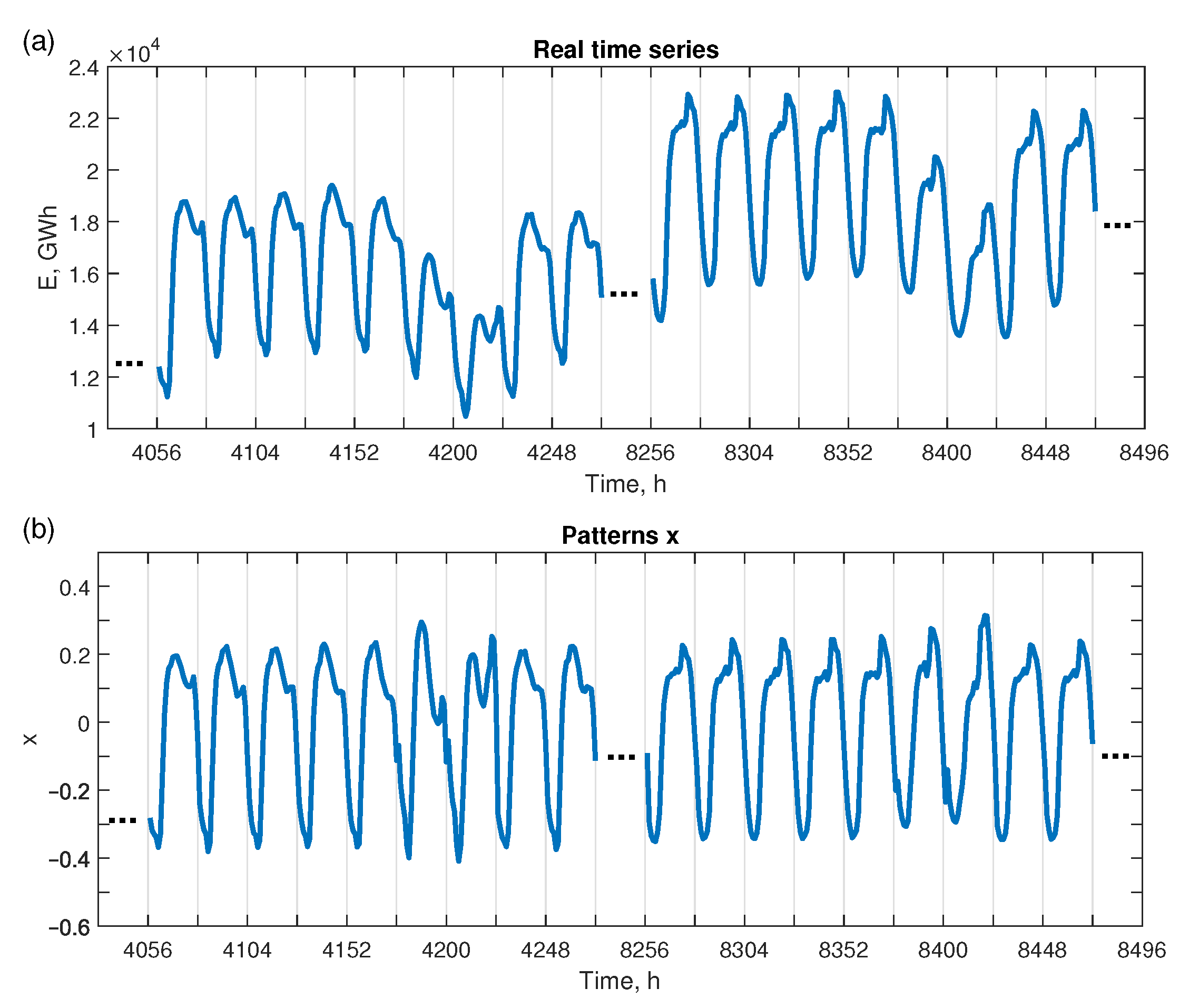
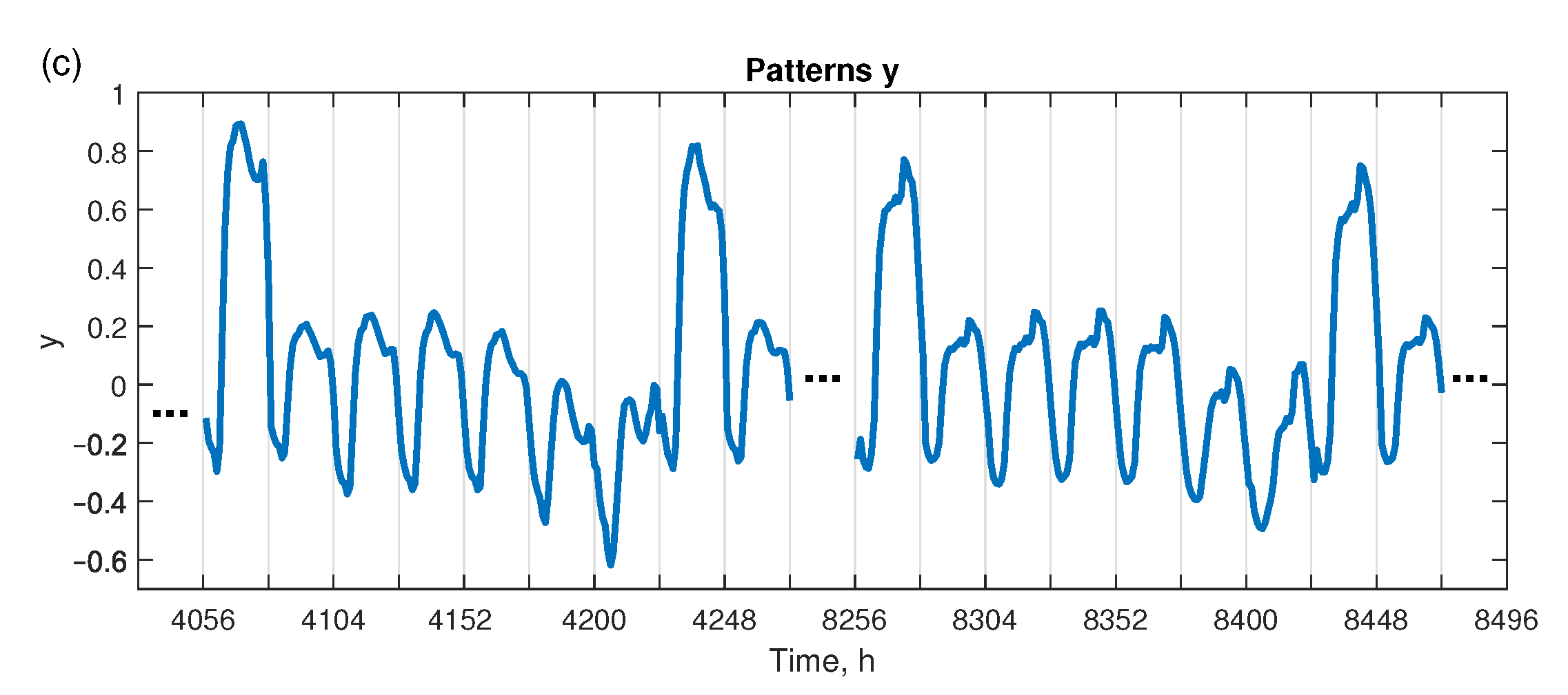
Figure 4 depicts the real hourly electricity demand TS and its x- and y-patterns for $\tau =1$. The upper panel shows two 9-day fragments of the original TS from June and December, respectively. These fragments differ in level due to annual seasonality. The daily sequences within these fragments differ in level as well due to the weekly seasonality. The pattern representation allows the model to deal with differences in level as well as variance in TS. Note that the x-patterns are all normalized and differ only in shape. The y-patterns, due to the use of coding variables from the previous periods, reveal the weekly seasonality. The y-patterns of Mondays are much higher than the patterns of other days of the week because the Monday sequences are coded with the means of Sunday sequences, which are much lower than the means of Monday sequences. For similar reasons, y-patterns for Saturdays and Sundays are lower than y-patterns for the other days of the week. Thus, the y-patterns are not unified globally but are unified in groups composed of the same days of the week. For this reason, we construct forecasting models that learn from data representing the same days of the week. For example, when we train the model for forecasting daily sequence for Monday, a training set for it is composed of the y-patterns representing all Mondays from history and the corresponding x-patterns representing the previous days (depending on the forecast horizon; Sundays for $\tau =1$).

3. Forecasting Model

The separate forecasting neural model is constructed for each day of the test period (e.g., one-year period). It learns on a training set composed of pairs of corresponding x- and y-patterns, where the x-patterns represent the same day of the week as the query test pattern: $\Psi ={\left\{({\mathbf{x}}_i,{\mathbf{y}}_i)\right\}}_{i=1}^N$, ${\mathbf{x}}_i,{\mathbf{y}}_i\in {\mathbb{R}}^n$. To obtain the forecasted y-pattern for the given day of the test period, the x-pattern representing previous day is presented to the trained network. We call this x-pattern a query test pattern. Query test pattern $\mathbf{x}$ is also used for weighting the training x-patterns, i.e., the training x-patterns that are the most similar to the query pattern have higher error weights and thus larger impacts on the loss function value. This is explained below in detail.

Note that, in our approach, we only use historical load values as inputs, i.e., vectors $\mathbf{x}$, which encode the daily TS sequences (24 values that encode loads in consecutive hours of the day). We do not use exogenous variables such as weather variables (temperature, wind speed, cloud cover, humidity, and precipitation) as their values are unknown for the forecast period (day $i+\tau$). Due to the pattern representation of TS and local approach (a specific training set and a separate model for each forecasting task), our proposed method does not require additional input variables indicating the day of the week, hour of the day, or period of the year. Thus, the model maps n-dimensional input vector space, $X={\mathbb{R}}^n$, into n-dimensional output vector space, $Y={\mathbb{R}}^n$.

To model the relationship between n-dimensional input and output patterns, we use a feedforward NN with a single hidden layer. The hidden layer consists of m hyperbolic tangent sigmoid nodes while the output layer consists of n linear nodes. To prevent overfitting, we use an early stopping. The number of hidden layers and nodes correspond to the target function complexity. In our case, we simplify the forecasting problem using pattern representation, which means we can limit NN architecture to a shallow, narrow one. This implies fast and more efficient training.

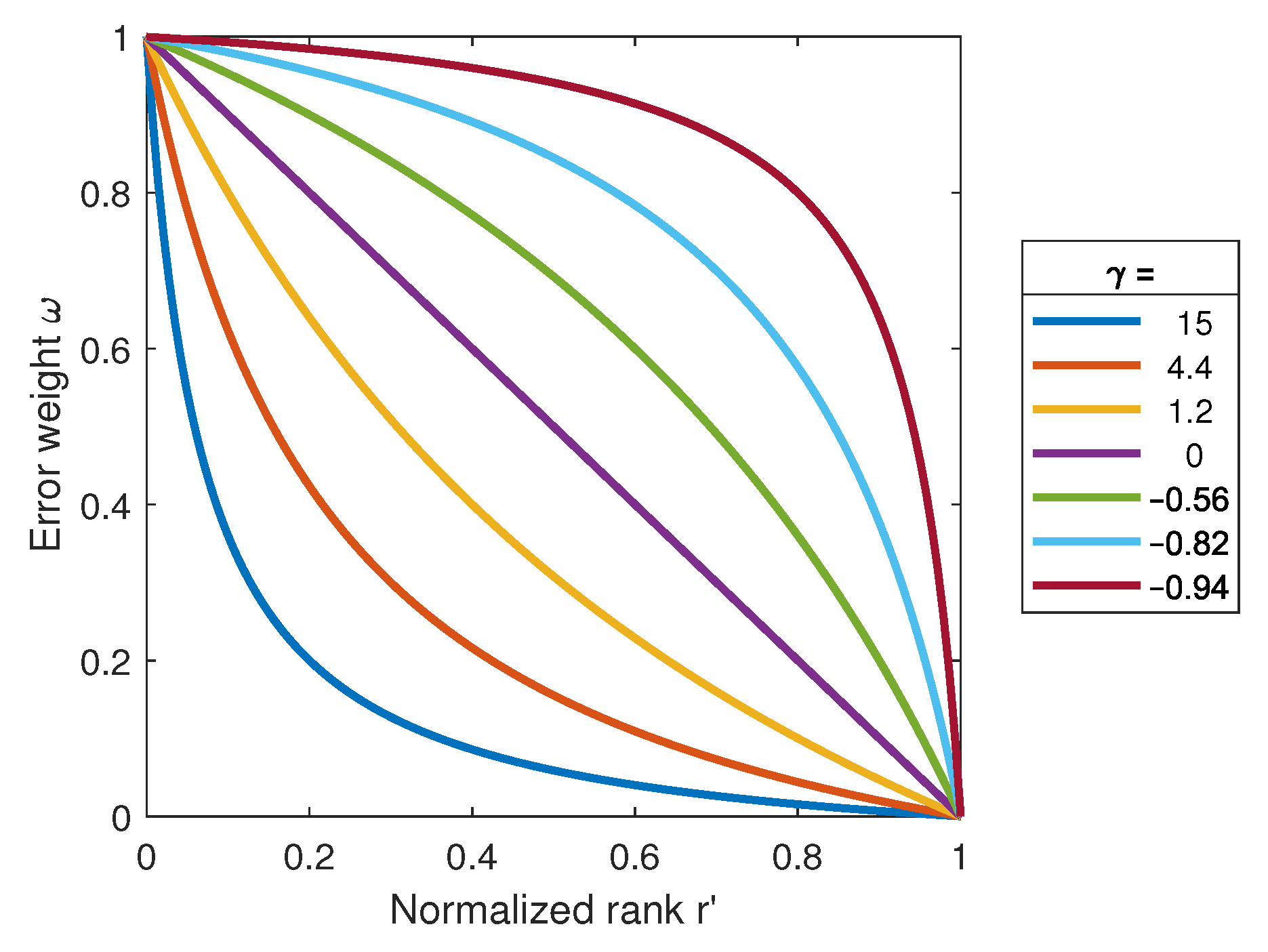
To improve the learning performance of NN, we introduce error weights to the mean square error loss function. The weights are assigned to the training samples. The weight value is dependent on the similarity between the training x-pattern and the query test pattern. More specifically, the weight value is proportional to the rank of the training x-pattern in the similarity ranking.

The weighted loss function is of the following form:

$$MSEw=\frac{1}{Nn}\sum _{i=1}^N{\omega }_i\sum _{t=1}^n{(y_{i,t}-{\widehat{y}}_{i,t})}^2$$

(4)

where $y_{i,t}$ and ${\widehat{y}}_{i,t}$ are the real and forecasted values, respectively, and ${\omega }_i$ is an error weight for ith training sample calculated as follows:

$${\omega }_i=\frac{1-r_i^{\prime }}{1+\gamma r_i^{\prime }}$$

(5)

where $r_i^{\prime }=\frac{r_i-1}{N-1}$ is a normalized rank; $r_i=1,\dots ,N$ is an ith training sample position in the distance from the test sample ranking; and $\gamma$ is a parameter controlling the weighting function shape.

The normalized rank takes the values $r_1^{\prime }=0$ for the nearest training sample to the query test sample, $r_2^{\prime }=\frac{1}{N-1}$ for the second nearest training sample, and $r_N^{\prime }=1$ for the furthest training sample. The distance between samples is calculated as an Euclidean distance between query test pattern $\mathbf{x}$ and training pattern ${\mathbf{x}}_i$ (as x-patterns are normalized vectors, a dot product ${\mathbf{x}}^T{\mathbf{x}}_i$ can be used instead of the Euclidean metric).

Figure 5 shows the weighting function (5) with different values of $\gamma$. For $\gamma =15$, the weights decrease rapidly with rank. In this case, only 20% of training samples have error weights over 0.2. For $\gamma =4.4$, 30% of training samples have error weights over 0.3. For $\gamma =0$, the error weighting function is linear. For $\gamma =-0.94$, 80% of training samples have error weights over 0.8. When we assume $\gamma =-1$ in Equation (2), the error weights for all training samples are the same, i.e., equal to one. The $\gamma$ hyperparameter controls the weighting of the training samples. In the experimental part of this work, we adjust its value to the test samples.

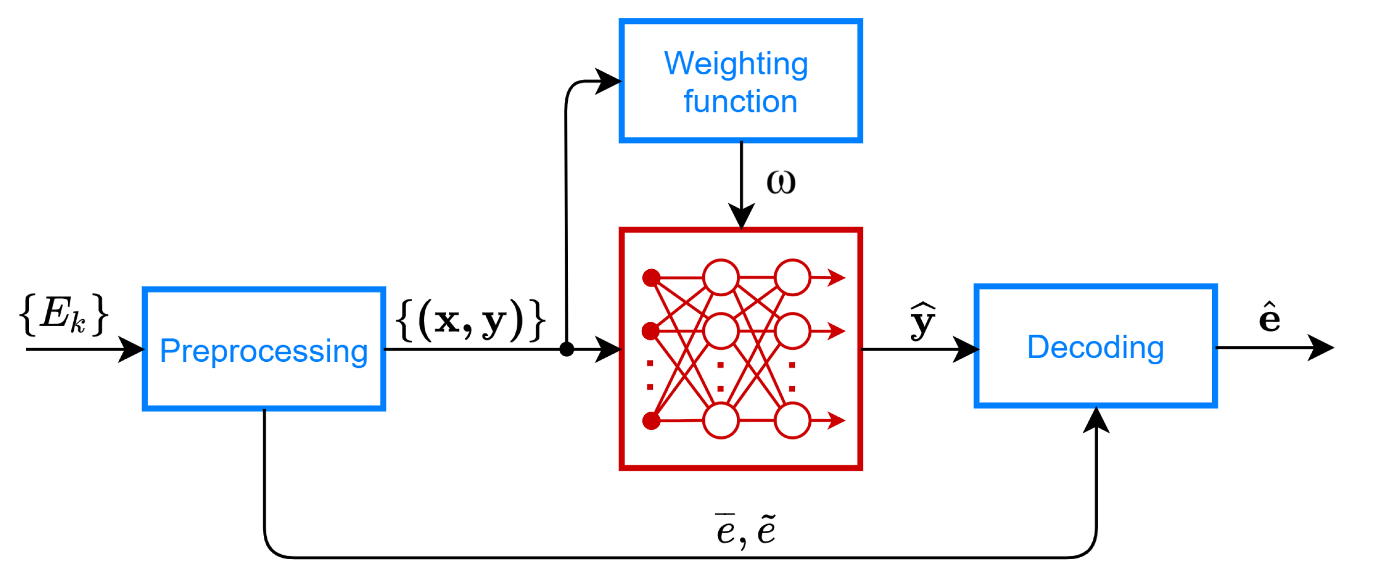
A block diagram of the proposed model is presented in Figure 6. From the raw TS, $\left\{E_k\right\}$, the preprocessing module produces a training set composed of x- and y-patterns. It also produces the query test pattern and coding variables for the forecasted y-pattern. The weighting function calculates the distances between training samples and the query test pattern, ranks the training samples, and calculates error weights for them. The NN learns on the training set using weights $\omega$ for weighting the individual training sample errors. It produces the forecast for the query test pattern. This forecast is decoded using Equation (3) into the real TS forecast using coding variables, $\overline{e}$ and $\tilde{e}$, determined from the most recent historical seasonal period (the period represented by the query test pattern).

4. Simulation Study

In this section, we present our experimental results for STLF. We use real-world data collected from www.entsoe.eu, (accessed on 6 April 2016), which details the hourly power system load in the period 2012–2015 for four countries: Poland (PL), Great Britain (GB), France (FR), and Germany (DE). We exclude atypical days such as public holidays (between 10 and 20 days a year) from these data. A one day-ahead forecasting problem is considered. We forecast the daily load profile for each day of 2015, training NN on previous data. For each forecasted day, a new NN is trained. The quality of forecasts was measured using metrics shown in

Table 2. Quality metrics of the forecasts.

Metric	Equation
Percentage Error	$PE=100\frac{(E-\widehat{E})}{E}$
Mean Percentage Error	$MPE=\frac{1}{K}{\sum }_{k=1}^K$${PE}_k$
Absolute Percentage Error	APE $=|PE|$
Mean Absolute Percentage Error	$MAPE=\frac{1}{K}{\sum }_{k=1}^K$${APE}_k$
Standard deviation of Percentage Error	Std(PE) $=\sqrt{\frac{1}{K}{\sum }_{k=1}^K{({PE}_k-MPE)}^2}$
Root Mean Square Error	$RMSE=\sqrt{\frac{1}{K}{\sum }_{k=1}^K{(E_k-{\widehat{E}}_k)}^2}$

where $E$ and $\widehat{E}$ are the real and forecasted hourly loads, respectively.

.

4.1. Tuning of the Error Weights

In the first study, we assumed a fixed NN architecture: 24 inputs, 24 hidden nodes, and 24 outputs. We used a hyperbolic tangent sigmoid transfer function in the hidden layer and a linear transfer function in the output layer. Early stopping was used to improve generalization: 20% of the training data was treated as a validation set for error monitoring during the learning process and halting when no reduction in validation error was observed. The network was trained using a Levenberg–Marquardt optimizer for 100 epochs.

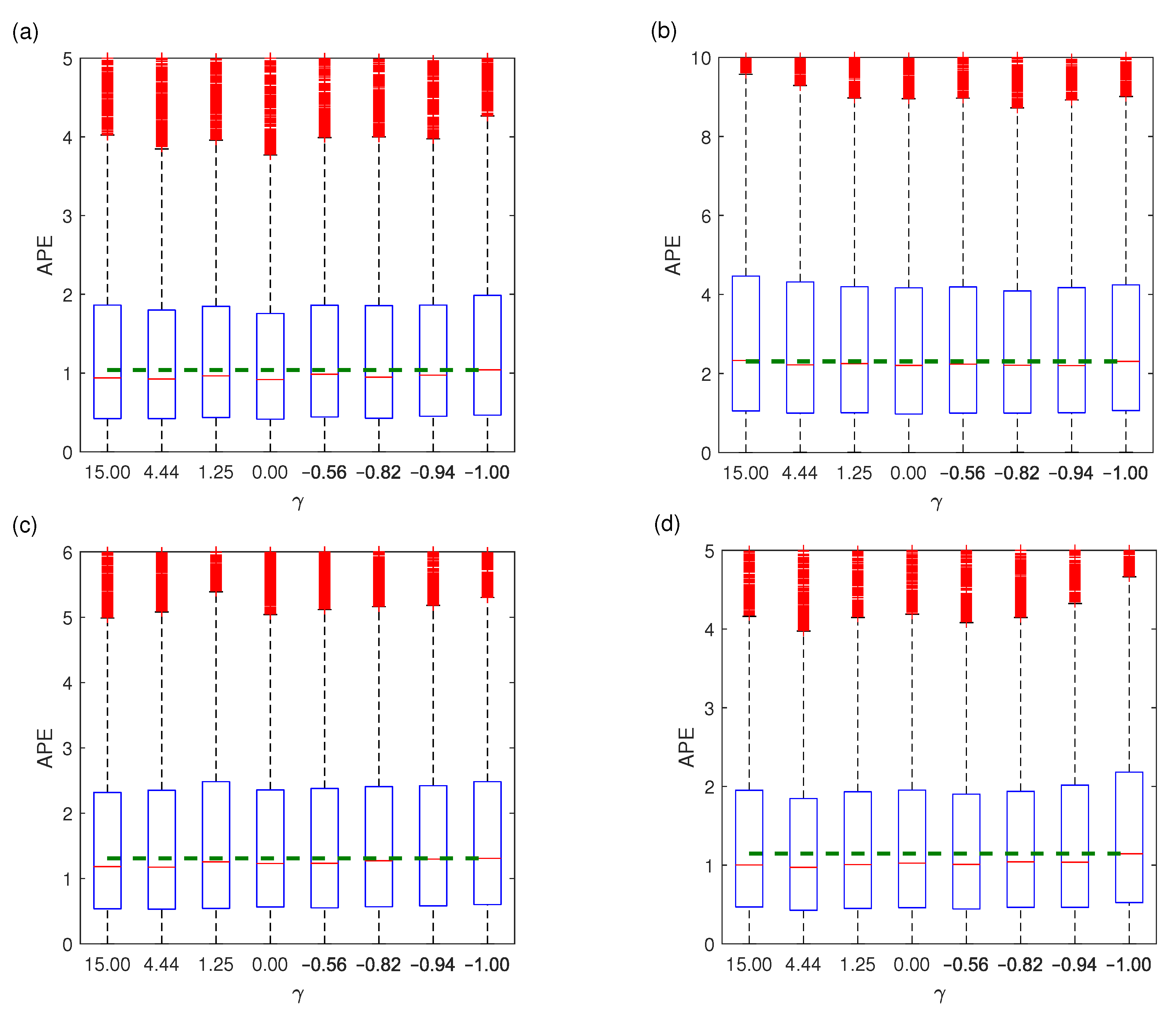
To assess the impact of the error weighting on the forecasting errors, for each $\gamma \in \Gamma =\{15,4.44,1.25,0,-0.56,-0.82,-0.94,-1\}$, where the last value corresponds to the learning variant without weighting, we train NNs and record test absolute percentage errors (APE). Distributions of these errors expressed by boxplots are depicted in Figure 7. The dashed horizontal lines express medians of APE for the baseline variants without weighting ($\gamma =-1$). As can be seen from the figure, weighting of errors in almost all cases leads to lower median of APE. The highest reduction in errors is for DE and PL. The lowest is for GB.

In the next experiment, we select the $\gamma$-value for each test pattern on the training sets. Four variants of learning mode were considered:

V1 

learning without error weighting as a baseline for other variants;

V2 

learning with error weighting, where $\gamma$ was selected on the training set, i.e., NN was trained for each $\gamma \in \Gamma$, and the minimal training error indicated the selected $\gamma$ value. NN with this $\gamma$ value was used to produce the forecast for the test pattern;

V3 

similar to V2, but $\gamma$ was selected on the five training patterns most similar to the query test pattern. First, the subset $\Phi$ of five training patterns closest (Euclidean distance) to the test pattern was selected. After NN training with $\gamma \in \Gamma$, average errors for $\Phi$ were calculated. The lowest error indicated the selected $\gamma$ value. Then, NN with this $\gamma$ was used to produce the forecast for the query test pattern; and

V4 

learning with fixed $\gamma =0$.

In variants V2 and V3, the value of $\gamma$ was searched individually for each test pattern. Set $\Phi$ in V3 represents the neighborhood of the test pattern. We expect that the $\gamma$ value selected as optimal for this neighborhood brings better results for the test pattern than the $\gamma$ value selected as optimal for all training patterns. V4 represents linear error weighting.

The forecasting quality metrics for the test data are presented in

Table 3. Results for PL data.

	V1 without Error Weighting	V2 with $\mathit{\gamma }$ Selected on Training Set	V3 with $\mathit{\gamma }$ Selected on $\mathbf{\Phi }$ Set	V4 with Linear Weighting $\mathit{\gamma }=0$
MAPE	1.48	1.35	1.35	1.28
Median (APE)	1.00	0.90	0.90	0.88
RMSE	471	397	378	357
MPE	0.33	0.28	0.29	0.29
Std (PE)	2.51	2.20	2.06	2.00

,

Table 4. Results for GB data.

	V1 without Error Weighting	V2 with $\mathit{\gamma }$ Selected on Training Set	V3 with $\mathit{\gamma }$ Selected on $\mathbf{\Phi }$ Set	V4 with Linear Weighting $\mathit{\gamma }=0$
MAPE	3.02	3.14	3.15	2.95
Median (APE)	2.25	2.19	2.19	2.16
RMSE	1354	1472	1488	1330
MPE	−0.57	−0.46	−0.41	−0.43
Std (PE)	4.13	4.46	4.51	4.08

,

Table 5. Results for FR data.

	V1 without Error Weighting	V2 with $\mathit{\gamma }$ Selected on Training Set	V3 with $\mathit{\gamma }$ Selected on $\mathbf{\Phi }$ Set	V4 with Linear Weighting $\mathit{\gamma }=0$
MAPE	1.87	1.82	1.80	1.81
Median (APE)	1.28	1.19	1.15	1.21
RMSE	1582	1659	1603	1582
MPE	−0.42	−0.26	−0.39	−0.31
Std (PE)	2.89	2.95	2.89	2.86

and

Table 6. Results for DE data.

	V1 without Error Weighting	V2 with $\mathit{\gamma }$ Selected on Training Set	V3 with $\mathit{\gamma }$ Selected on $\mathbf{\Phi }$ Set	V4 with Linear Weighting $\mathit{\gamma }=0$
MAPE	1.64	1.50	1.54	1.50
Median (APE)	1.10	0.95	0.95	0.99
RMSE	1503	1574	1647	1474
MPE	−0.02	0.07	−0.04	0.05
Std (PE)	2.54	2.73	2.84	2.55

. They include the mean absolute percentage error (MAPE), median of APE, root mean square error (RMSE), mean percentage error (MPE), and standard deviation of percentage error (Std(PE)) as a measure of the forecast dispersion.

To confirm that the results from the four learning variants are significantly different, we performed a Wilcoxon signed-rank test with $\alpha =0.05$ for APE. The diagrams in Figure 8 depict pairwise comparisons of the learning variants. The arrow lying at the intersection of the two variants indicates which of them gave the significantly lower error. A lack of an arrow means that both variants gave statistically indistinguishable errors.

From Table 3, Table 4, Table 5 and Table 6 and Figure 8, we can conclude the following:

• The baseline variant V1 gave significantly higher errors than other variants in 10 out of 12 cases.
• V4 gave significantly lower errors than the baseline variant V1 for all data sets. It also beat its competitors, V2 and V3, for PL and GB data.
• V2 and V3 gave lower errors than the baseline variant for PL, FR, and DE.
• V3 gave the significantly lowest APE for FR data.

MPE shown in Table 3, Table 4, Table 5 and Table 6 allows us to compare the bias of the forecasts produced by the different model variants. A positive value of MPE indicates underprediction, while a negative value indicates overprediction. As can be seen from the tables, for PL data, the bias was positive, whilst for GB and FR data, it was negative. For these three data sets, error weighting yielded a positive effect on the bias reduction: by up to 15% for PL, 28% for GB, and 35% for FR. For DE data, we can observe very low bias regardless of the model variant.

4.2. Tuning of the Number of Hidden Nodes

In a further experiment, we change the NN architecture. We consider a variable number of hidden nodes from 2 to 48. Based on the results of previous experiments, we restrict this study to NN with the linear error weighting function ($\gamma =0$). For each test sample, we select the number of the hidden nodes in two ways: (1) on the training set and (2) on the $\Phi$ set of five training patterns closest to the test pattern. The results for both cases are shown in

Table 7. Results for a variable number of hidden nodes.

	PL	GB	FR	DE
MAPE for m selected on training set	1.44	3.28	1.97	1.56
MAPE for m selected on $\Phi$ set	1.33	3.26	1.87	1.49
MAPE for $m=n=24$	1.34	3.11	1.77	1.45
MAPE for $m=n/2=12$	1.29	2.91	1.73	1.43

(due to the different training sessions, the results for $m=n=24$ differ from those presented in Table 3, Table 4, Table 5 and Table 6). As can be seen from this table, the selection of the optimal number of hidden nodes on the training set or on the $\Phi$ set does not improve significantly the results for the baseline variant with fixed $m=n=24$.

Figure 9 shows the mean test errors depending on the number of hidden nodes m. As can be seen from this figure, for all countries, the error initially decreases with m and then begins to increase. This increase in error is due to overfitting, i.e., the complexity of the model is greater than the complexity of the relationship it approximates. The lowest mean test errors for each country were achieved for $m=16$ for PL, $m=14$ for GB, $m=8$ for FR, and $m=10$ for DE. Thus, assuming $m=n=24$ is not the best choice.

When deciding on the optimal number of hidden nodes for a given TS, we can consider the results for similar TS. Doing so, we can assume the hidden nodes for PL as the mean best m value for other countries, i.e., $(14+8+10)/3\approx 11$. Using this approach for other countries, we obtain $m\approx 11$ for GB and $m\approx 13$ for FR and DE. Thus, the number of hidden nodes is near $m=n/2=12$. Let us assume such a value of m for simplicity. The errors for $m=n/2=12$ are presented in the last row of Table 7. As you can see, this case turned out to be slightly better than the baseline variant.

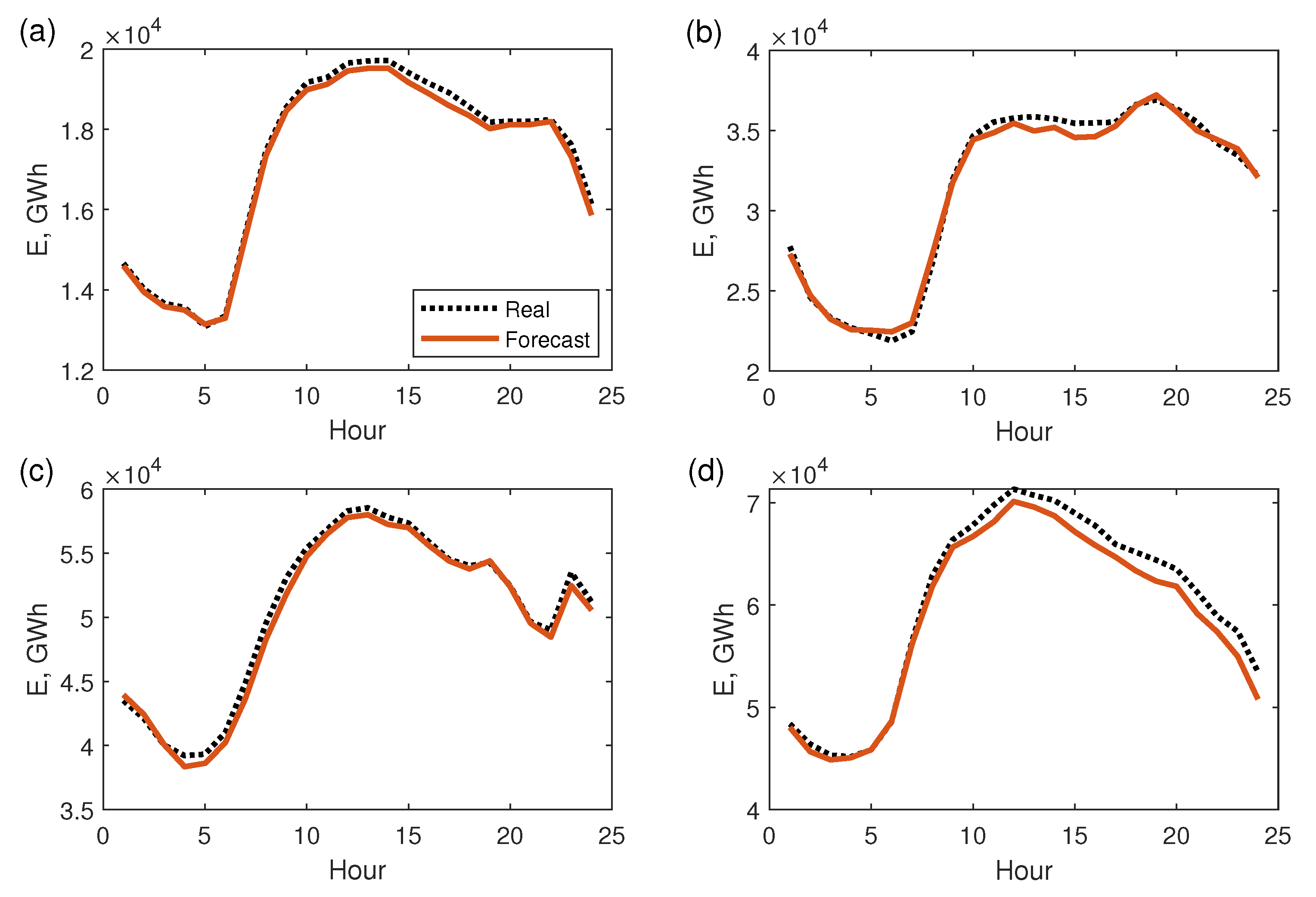
Figure 10 shows examples of forecasts of the daily load profiles produced by proposed model with $m=12$ hidden nodes and linear error weighting. Note that the proposed model produces a multi-output response, maintaining the relationships between the output variables (y-pattern components). In the case of single-output models, these relationships are ignored because the variables are predicted independently. This may cause a lack of smoothness in the forecasted curve (zigzag effect).

4.3. Discussion

From the experimental part of this work, we can conclude that linear error weighting and $m=n/2$ can be considered the default settings for the multi-output pattern-based NN forecasting models. With respect to the model without weighting, such settings provide a relative gain in terms of MAPE of 13% for PL, 4% for GB, 7% for FR, and 13% for DE.

In our earlier work [25], we compared different NN architectures for STLF: multilayer perceptron (MLP), radial basis function NN, generalized regression NN (GRNN), two variants of fuzzy counterpropagation NNs, and three variants of self-organizing maps. Among them, MLP (architecture used also in this study) turned out to be one of the most accurate. It outperformed all other models except GRNN. The forecasting errors (MAPE) averaged over four STLF tasks were $1.92$ for MLP, $1.85$ for GRNN, and over $2.00$ for other neural models (for comparison, the naive forecast error was $MAPE=4.14$). MLP outperformed also classical statistical models such as ARIMA ($MAPE=2.46$) and ETS ($MAPE=2.28$).

In [23], the local and global variants of MLP were compared with other state-of-the-art STLF models such as principal components regression, partial least-squares regression (PLSR), Nadaraya–Watson estimator (N–WE), fuzzy neighborhood model (FNM), two models based on k-means clustering, and three models using artificial immune systems. The local variant of MLP (corresponding to the model used in this study) turned out to be one of the most accurate. It was beaten only by three models: PLSR ($MAPE=1.82$), N–WE ($MAPE=1.83$), and FNM ($MAPE=1.89$). The empirical comparison of MLP with classical statistical models as well as state-of-the-art ML models reported in [23,25] shows its high performance in STLF. This performance can be further improved by using the pattern similarity-based error weighting, as shown in this study.

The proposed forecasting framework can be useful not only for STLF but also for a broad range of complex TS forecasting problems. To capture many seasonal cycles, the nonlinear trend, and long-term dependencies, our approach does not require a complex, deep architecture equipped with sophisticated mechanisms such as dilation, attention, dropout, and residual connections (in fact, some of these mechanisms are used not to improve the forecast accuracy but to enable effective learning of the deep NN). Unlike deep learning, which is very computationally intensive, our approach does not require powerful hardware for learning its single-hidden layer model. Moreover, our approach has a more transparent architecture than deep NNs, its working principle is more understandable, and it has far fewer parameters to fine-tune than its deep competitors. By using patterns for data representation, our approach solves many problems related to complex forecasting tasks. Note also that, in our approach, we avoid TS decomposition and forecasting each TS component separately. Thus, the construction, optimization, and learning of the forecasting model are faster. Producing a vector output, the proposed model is able to multi-step forecast without a recursive approach. The components of the output pattern are the forecasts for the successive time periods. The model is also able to produce forecasts for further horizons. In such a case, we define output patterns in an appropriate way (with $\tau >1$).

The forecasting model using a pattern-based representation of TS described in this study was developed for seasonal TS. An application of this model to forecasting non-seasonal series requires further research. The proposed approach with weighted loss function (4) is based on the assumption that, if pattern ${\mathbf{x}}_a$ is similar to pattern ${\mathbf{x}}_b$, then pattern ${\mathbf{y}}_a$ is similar to pattern ${\mathbf{y}}_b$. This assumption can be verified for a given TS using appropriate statistical tests, i.e., the chi-squared test (see [24]). If the test does not confirm this assumption, the weighted loss function may not improve the results. In such a case, we can look for another method of TS representation or coding. For example, in [46], to improve the performance of the models with pattern-based representation, the coding variables for y-patterns, $\overline{e}$ and $\tilde{e}$ in Equation (2), were not determined from preceding period i but were predicted for period $i+\tau$. This resulted in a significant reduction in forecast errors.

The proposed model is a univariate forecasting model, but exogenous variables can be easily introduced as additional NN inputs. As with endogenous variables, a key problem with exogenous variables is their appropriate representation.

5. Conclusions

Forecasting TS with multiple seasonality such as STLF is a challenging problem requiring the forecasting model to be equipped with appropriate mechanisms to deal with multiple seasonal cycles. In this study, we use an alternative approach to deal with multiple seasonality. It involves TS preprocessing to filter out the trend and seasonal cycles longer that the basic cycle. This simplifies the relationship between input and output variables. To model this relationship, we use multi-output shallow NN architecture. To improve the learning performance of the model, we propose using the loss function with error weights. The error weights are assigned to the training samples and express their similarity to the query test pattern. This approach leads to more accurate modeling of the target function in the neighborhood of the test pattern. The empirical study, including a challenging STLF problem for four European countries, showed the improvement in performance for our proposed approach over standard NN learning without error weighting.

The proposed approach using a simple single-hidden layer NN is an alternative to deep NN solutions, which have been developed rapidly for forecasting problems in recent years. Unlike deep architectures, it is simple, transparent, easily tuned, and fast trained. To further simplify the model and learning process, in our future work, we plan to employ randomization-based NNs to complex forecasting problems.

References

1. Sowinski, J. The Impact of the Selection of Exogenous Variables in the ANFIS Model on the Results of the Daily Load Forecast in the Power Company. Energies 2021, 14, 345. [Google Scholar] [CrossRef]
2. Parol, M.; Piotrowski, P.; Kapler, P.; Piotrowski, M. Forecasting of 10-Second Power Demand of Highly Variable Loads for Microgrid Operation Control. Energies 2021, 14, 1290. [Google Scholar] [CrossRef]
3. Popławski, T.; Szeląg, P.; Bartnik, R. Adaptation of models from determined chaos theory to short-term power forecasts for wind farms. Bull. Pol. Acad. Sci. Tech. Sci. 2020, 68, 1491–1501. [Google Scholar] [CrossRef]
4. Trull, O.; García-Díaz, J.C.; Peiró-Signes, A. Forecasting Irregular Seasonal Power Consumption. An Application to a Hot-Dip Galvanizing Process. Appl. Sci. 2021, 11, 75. [Google Scholar] [CrossRef]
5. Box, G.E.P.; Jenkins, G.M.; Reinsel, G.C. Time Series Analysis: Forecasting and Control, 3rd ed.; Prentice Hall: Englewood Cliff, NJ, USA, 1994. [Google Scholar]
6. Taylor, J.W. Short-term electricity demand forecasting using double seasonal exponential smoothing. J. Oper. Res. Soc. 2003, 54, 799–805. [Google Scholar] [CrossRef]
7. Taylor, J.W. Triple seasonal methods for short-term load forecasting. Eur. J. Oper. Res. 2010, 204, 139–152. [Google Scholar] [CrossRef] [Green Version]
8. Gould, P.G.; Koehler, A.B.; Ord, J.K.; Snyder, R.D.; Hyndman, R.J.; Vahid-Araghi, F. Forecasting time-series with multiple seasonal patterns. Eur. J. Oper. Res. 2008, 191, 207–222. [Google Scholar] [CrossRef]
9. De Livera, A.M.; Hyndman, R.J.; Snyder, R.D. Forecasting time series with complex seasonal patterns using exponential smoothing. J. Am. Stat. Assoc. 2011, 106, 1513–1527. [Google Scholar] [CrossRef] [Green Version]
10. Taylor, S.J.; Letham, B. Forecasting at scale. Am. Stat. 2018, 72, 37–45. [Google Scholar] [CrossRef]
11. Benidis, K.; Rangapuram, S.S.; Flunkert, V.; Wang, B.; Maddix, D.; Turkmen, C.; Gasthaus, J.; Bohlke-Schneider, M.; Salinas, D.; Stella, L.; et al. Neural forecasting: Introduction and literature overview. arXiv 2020, arXiv:2004.10240. [Google Scholar]
12. Smyl, S. A hybrid method of exponential smoothing and recurrent neural networks for time series forecasting. Int. J. Forecast. 2020, 36, 75–85. [Google Scholar] [CrossRef]
13. Bandara, K.; Bergmeir, C.; Hewamalage, H. LSTM-MSNet: Leveraging forecasts on sets of related time series with multiple seasonal patterns. IEEE Trans. Neural Netw. Learn. Syst. 2021, 32, 1586–1599. [Google Scholar] [CrossRef] [Green Version]
14. Salinas, D.; Flunkert, V.; Gasthaus, J.; Januschowski, T. DeepAR: Probabilistic forecasting with autoregressive recurrent networks. Int. J. Forecast. 2020, 36, 1181–1191. [Google Scholar] [CrossRef]
15. Oreshkin, B.N.; Carpov, D.; Chapados, N.; Bengio, Y. N-BEATS: Neural basis expansion analysis for interpretable time series forecasting. In Proceedings of the 8th International Conference on Learning Representations, ICLR, Addis Ababa, Ethiopia, 26–30 April 2020. [Google Scholar]
16. Li, S.; Jin, X.; Xuan, Y.; Zhou, X.; Chen, W.; Wang, Y.-X.; Yan, X. Enhancing the locality and breaking the memory bottleneck of transformer on time series forecasting. In Proceedings of the Advances in Neural Information Processing Systems (NeurIPS), Vancouver, BC, Canada, 8–14 December 2019. [Google Scholar]
17. Vaswani, A.; Shazeer, N.; Parmar, N.; Uszkoreit, J.; Jones, L.; Gomez, A.N.; Kaiser, Ł.; Polosukhin, I. Attention is all you need. In Proceedings of the Advances in Neural Information Processing Systems (NIPS), Long Beach, CA, USA, 4–9 December 2017; pp. 5998–6008. [Google Scholar]
18. Ghaderpour, E.; Vujadinovic, T. Change Detection within Remotely Sensed Satellite Image Time Series via Spectral Analysis. Remote Sens. 2020, 12, 4001. [Google Scholar] [CrossRef]
19. Torrence, C.; Compo, G.P. A Practical Guide to Wavelet Analysis. Bull. Am. Meteorol. Soc. 1998, 79, 61–78. [Google Scholar] [CrossRef] [Green Version]
20. Chen, D.; Zhang, J.; Jiang, S. Forecasting the Short-Term Metro Ridership With Seasonal and Trend Decomposition Using Loess and LSTM Neural Networks. IEEE Access 2020, 8, 91181–91187. [Google Scholar] [CrossRef]
21. Zhang, Z.; Hong, W.C. Electric load forecasting by complete ensemble empirical mode decomposition adaptive noise and support vector regression with quantum-based dragonfly algorithm. Nonlinear Dyn. 2019, 98, 1107–1136. [Google Scholar] [CrossRef]
22. Dudek, G. Forecasting daily load curves of power system using radial basis function neural networks. In Proceedings of the 10th Conference Present-Day Problems in Power Engineering, APE 2001, Gdansk–Jurata, Poland, 6–8 June 2001; Volume 3, pp. 93–100. (In Polish). [Google Scholar]
23. Dudek, G. Multilayer perceptron for short-term load forecasting: From global to local approach. Neural Comput. Appl. 2019, 32, 3695–3707. [Google Scholar] [CrossRef] [Green Version]
24. Dudek, G. Pattern Similarity-based Methods for Short-term Load Forecasting—Part 1: Principles. Appl. Soft Comput. 2015, 37, 277–287. [Google Scholar] [CrossRef]
25. Dudek, G. Neural networks for pattern-based short-term load forecasting: A comparative study. Neurocomputing 2016, 205, 64–74. [Google Scholar] [CrossRef]
26. Dudek, G.; Pełka, P.; Smyl, S. A hybrid residual dilated LSTM and exponential smoothing model for mid-term electric load forecasting. IEEE Trans. Neural Netw. Learn. Syst. 2021. [Google Scholar] [CrossRef]
27. Kuster, C.; Rezgui, Y.; Mourshed, M. Electrical load forecasting models: A critical systematic review. Sustain. Cities Soc. 2017, 35, 257–270. [Google Scholar] [CrossRef]
28. Sidorov, D.; Tao, Q.; Muftahov, I.; Zhukov, A.; Karamov, D.; Dreglea, A.; Liu, F. Energy balancing using charge/discharge storages control and load forecasts in a renewable-energy-based grids. In Proceedings of the 38th Chinese Control Conference, Guangzhou, China, 27–30 July 2019; pp. 6865–6870. [Google Scholar]
29. Hippert, H.S.; Pedreira, C.E.; Souza, R.C. Neural networks for short-term load forecasting: A review and evaluation. IEEE Trans. Power Syst. 2001, 16, 44–55. [Google Scholar] [CrossRef]
30. Kodogiannis, V.S.; Anagnostakis, E.M. Soft computing based techniques for short-term load forecasting. Fuzzy Sets Syst. 2002, 128, 413–442. [Google Scholar] [CrossRef]
31. Zang, H.; Cheng, L.; Ding, T.; Cheung, K.; Liang, Z.; Wei, Z.; Sun, G. Hybrid method for short-term photovoltaic power forecasting based on deep convolutional neural network. IET Gener. Transm. Distrib. 2018, 12, 4557–4567. [Google Scholar] [CrossRef]
32. Kong, W.; Dong, Z.Y.; Jia, Y.; Hill, D.J.; Xu, Y.; Zhang, Y. Short term residential load forecasting based on LSTM recurrent neural network. IEEE Trans. Smart Grid 2019, 10, 841–851. [Google Scholar] [CrossRef]
33. Chen, K.; Chen, K.; Wang, Q.; He, Z.; Hu, J.; He, J. Short-Term Load Forecasting With Deep Residual Networks. IEEE Trans. Smart Grid 2019, 10, 3943–3952. [Google Scholar] [CrossRef] [Green Version]
34. Wang, L.; Zhang, Z.; Chen, J. Short-term electricity price forecasting with stacked denoising autoencoders. IEEE Trans. Power Syst. 2017, 32, 2673–2681. [Google Scholar] [CrossRef]
35. Shi, H.; Xu, M.; Li, R. Deep learning for household load forecasting—A novel pooling deep RNN. IEEE Trans. Smart Grid 2018, 9, 5271–5280. [Google Scholar] [CrossRef]
36. Rafiei, M.; Niknam, T.; Aghaei, J.; Shafie-Khah, M.; Catalao, J.P.S. Probabilistic load forecasting using an improved wavelet neural network trained by generalized extreme learning machine. IEEE Trans. Smart Grid 2018, 9, 6961–6971. [Google Scholar] [CrossRef]
37. Li, B.; Zhang, J.; He, Y.; Wang, Y. Short-term load-forecasting method based on wavelet decomposition with second-order gray neural network model combined with ADF test. IEEE Access 2017, 5, 16324–16331. [Google Scholar] [CrossRef]
38. Deihimi, A.; Orang, O.; Showkati, H. Short-term electric load and temperature forecasting using wavelet echo state networks with neural reconstruction. Energy 2013, 57, 382–401. [Google Scholar] [CrossRef]
39. Kulkarni, S.; Simon, S.P.; Sundareswaran, K. A spiking neural network (SNN) forecast engine for short-term electrical load forecasting. Appl. Soft Comput. 2013, 13, 3628–3635. [Google Scholar] [CrossRef]
40. Sadaei, H.J.; e Silva, P.C.d.L.; Guimaraes, F.G.; Lee, M.H. Short-term load forecasting by using a combined method of convolutional neural networks and fuzzy time series. Energy 2019, 175, 365–377. [Google Scholar] [CrossRef]
41. Sheng, Z.; Wang, H.; Chen, G.; Zhou, B.; Sun, J. Convolutional residual network to short-term load forecasting. Appl. Intell. 2021, 51, 2485–2499. [Google Scholar] [CrossRef]
42. Acharya, S.K.; Wi, Y.-M.; Lee, J. Short-Term Load Forecasting for a Single Household Based on Convolution Neural Networks Using Data Augmentation. Energies 2019, 12, 3560. [Google Scholar] [CrossRef] [Green Version]
43. Fernando, K.R.M.; Tsokos, C.P. Dynamically Weighted Balanced Loss: Class Imbalanced Learning and Confidence Calibration of Deep Neural Networks. IEEE Trans. Neural Netw. Learn. Syst. 2021. [Google Scholar] [CrossRef]
44. Zhang, K.; Wu, Z.; Yuan, D.; Luan, J.; Jia, J.; Meng, H.; Song, B. Re-Weighted Interval Loss for Handling Data Imbalance Problem of End-to-End Keyword Spotting. Proc. Interspeech 2020, 2567–2571. [Google Scholar] [CrossRef]
45. Rengasamy, D.; Jafari, M.; Rothwell, B.; Chen, X.; Figueredo, G.P. Deep Learning with Dynamically Weighted Loss Function for Sensor-Based Prognostics and Health Management. Sensors 2020, 20, 723. [Google Scholar] [CrossRef] [Green Version]
46. Dudek, G.; Pełka, P. Pattern similarity-based machine learning methods for mid-term load forecasting: A comparative study. Appl. Soft Comput. 2021, 104, 107223. [Google Scholar] [CrossRef]
Figure 1. Periodograms of the hourly load TS for PL (a), GB (b), FR (c), and DE (d). Dashed lines indicate 12 h, daily, weekly, and annual periodicity.
Energies 14 03224 g001
Figure 2. Hourly electricity demand TS for Poland, (a) 4-year period, (b) weekly periods.
Energies 14 03224 g002
Figure 3. Magnitudes of the seasonal components in the hourly electricity demand TS for Poland.
Energies 14 03224 g003
Figure 4. Real hourly electricity demand TS (a) and its x- (b) and y-patterns (c).
Energies 14 03224 g004aEnergies 14 03224 g004b
Figure 5. An error weighting function.
Energies 14 03224 g005
Figure 6. Block diagram of the proposed NN forecasting model.
Energies 14 03224 g006
Figure 7. Distribution of APE depending on γ for PL (a), GB (b), FR (c), and DE (d). The red lines in the boxes are the medians, and the green dashed line is the median for the baseline variant.
Energies 14 03224 g007
Figure 8. Results of the Wilcoxon signed-rank test for APE.
Energies 14 03224 g008
Figure 9. Test error depending on the number of hidden nodes.
Energies 14 03224 g009
Figure 10. Examples of forecasts for PL (a), GB (b), FR (c), and DE (d).
Energies 14 03224 g010