Level Crossing Barrier Machine Faults and Anomaly Detection with the Use of Motor Current Waveform Analysis

Abstract

Barrier machines are a key component of automatic level crossing systems ensuring safety on railroad crossings. Their failure results not only in delayed railway transportation, but also puts human life at risk. To prevent faults in this critical safety element of automatic level crossing systems, it is recommended that fault and anomaly detection algorithms be implemented. Both algorithms are important in terms of safety (information on whether a barrier boom has been lifted/lowered as required) and predictive maintenance (information about the condition of the mechanical components). Here, the authors propose fault models for barrier machine fault and anomaly detection procedures based on current waveform observation. Several algorithms were applied and then assessed such as self-organising maps (SOM), autoencoder artificial neural network, local outlier factor (LOF) and isolation forest. The advantage of the proposed solution is there is no change of hardware, which is already homologated, and the use of the existing sensors (in a current measurement module). The methods under evaluation demonstrated acceptable rates of detection accuracy of the simulated faults, thereby enabling a practical application at the test stage.

1. Introduction

The main task of automatic level crossing systems is to ensure the safety of road users and approaching trains [1,2,3]. They must comply with the requirements of Safety Integrity Level 4 [4] as the consequences of the majority of incidents are usually very severe. According to the official statistical data for 2019 [5], there were 185 safety incidents related to level crossing systems in Poland and as a result 55 people were killed and 19 were severely wounded.

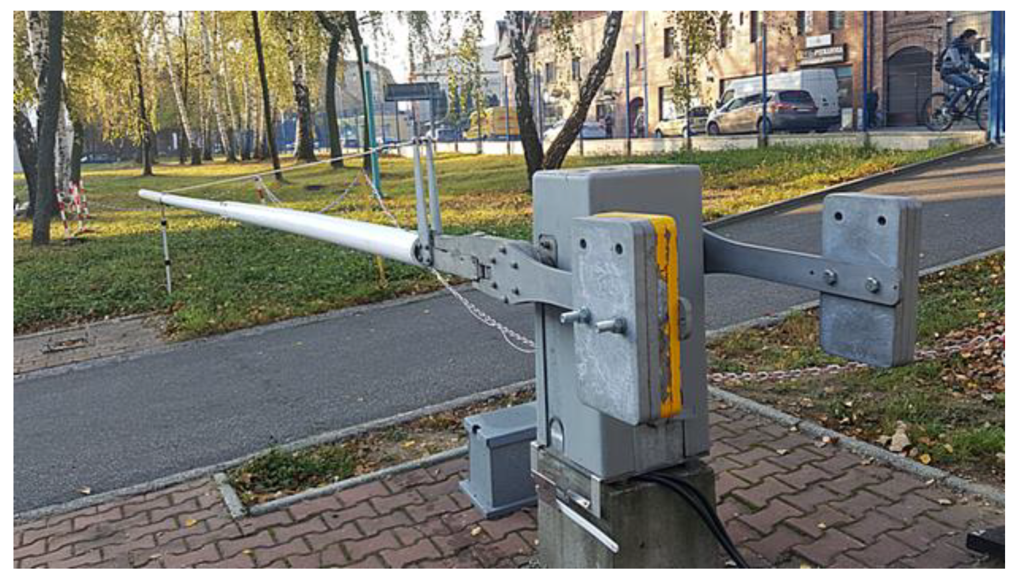
A barrier machine is one of the most important and widely used warning devices—a sample barrier machine is shown in Figure 1. It is required that barrier booms are lowered within a defined time interval after the pre-warning sequence is successfully completed. When the barrier booms are lowered, it is assumed that the road users are well protected against irresponsible entry to the level crossing area. This may appear an easy task, but it is very difficult to ensure near 100% reliability of barrier machines considering obstacle detection, fault diagnosis and predictive maintenance [6]. The idea of increasing the reliability of railway systems with the use of current waveform analysis and outlier detection algorithms is presented in the paper.

Predictive maintenance, classification of patterns of machine health and fault detection are significant aspects involved in developing innovative Industry 4.0 solutions [6,7]. Researchers from all over the world have put a strong emphasis on improving the reliability of manufacturing process. The common approach to estimating the reliability of systems based on DC motors is to analyse their input current and any readings that deviate from standard waveforms may indicate stall, overload, damage, or failure [8,9]. Scientists have developed numerous solutions for examining the health of machines or classifying faults detected in such systems. For example, current signature analysis is used in induction motors to provide valuable information on bottle capping failures [10]. Supply current analysis is also used in the automotive industry for examining the reliability of advanced driver-assistance systems (ADAS) modules [11].

Barrier machine design and functional requirements differ depending on the country of application. For the purpose of this research, requirements valid for two countries, i.e., Poland [9,10] and the United Kingdom [11] were taken into consideration. One of the important factors that has an impact on the testing scenario is the range of the angular movement of the boom. To ensure a stable upper position and provide self-falling capabilities, the barrier boom when lifted does not reach a fully vertical position. Similarly, in the case of the lower position, the boom cannot reach a fully horizontal position to enable adaptation to the road profile and ensure reliable operation. Considering these constraints, the movement range of the test stand was adjusted to be 80° in total.

In this paper, however, we put the emphasis on detecting anomalies of any kind, which either leads to estimating the degree of barrier machine wear or detecting their sudden damage [12]. Among all of the outlier detection algorithms, there are simple ones such as scalar comparison (e.g., aggregate of the whole waveform—a mean, a standard deviation, etc.), but there are also more sophisticated ones such as analysing feature vectors compared to the whole dataset. The vast majority of methods used for anomaly analysis are based on unsupervised learning, e.g., local outlier factor [13], isolation forest [14], one class support vector machine [15], robust covariance and autoencoder neural network [16]. These methods are trained using the whole population of data, and the models that are generated are capable of distinguishing between correct vectors and anomalies.

2. Fault Models

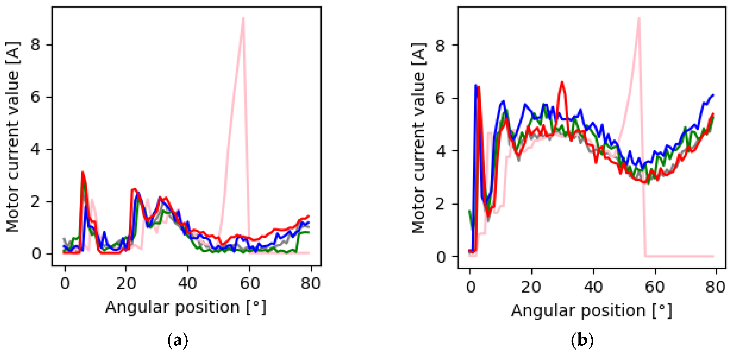
A barrier machine has a significant impact on overall safety and special attention must be paid to its reliability analysis. Therefore, based on experience and acquired data, a set of the most common faults was introduced. Four representative barrier machine faults were taken into consideration: (a) a boom hits a solid obstacle, (b) a boom hits a flexible obstacle, (c) a gear fault, and (d) white noise. All of the relevant representative current waveforms are shown in Figure 2. All these faults seriously disrupt barrier machine performance as the lowering of the barrier booms is delayed at the level crossing area. Consequently, train traffic is impacted by a faulty level crossing subsystem. The accumulated duration of the delay increases, thereby resulting in significant losses to the rail operator.

The exemplary vector of undistorted current waveform can be written as follows:

$$I=\left[i_1, i_2, \dots , i_{80}\right]$$

(1)

The whole dataset consists of N current waveforms, which is denoted by J:

$$J=\left[I_1; I_2; \dots ; I_N\right]$$

(2)

From (1) and (2), J can be written as follows:

$$J=\left[\begin{array}{ccc}{i}_{1,1}& \cdots & i_{1,80}\\ ⋮& \ddots & ⋮\\ i_{N,1}& \cdots & i_{N,80}\end{array}\right]$$

(3)

2.1. Boom Hits a Solid Obstacle

In this fault model it is assumed that the movement of the boom is stopped suddenly, for example, by hitting the roof of a car, (a fault model for a solid obstacle, FSO). The current in the barrier machine motor circuit increases following the growing tension of the boom, see the pink trace in Figure 2. Depending on the interface circuit structure, the overcurrent activates an overcurrent-circuit breaker or an electronic protection circuit. In the first case, the level crossing requires intervention by maintenance personnel. The resulting delay caused by a faulty barrier machine is significant. In the other case, a fully autonomous resolution of the problem is still possible. When an overcurrent occurs, the barrier machine is stopped and the boom can be raised again. After a defined period of time another attempt to lower it may be made.

$$i_{FSO,x}=\{\begin{array}{c}{i}_{rand\_int\left(1,N\right),x}\hspace{1em}if\hspace{1em}x<k_{FSO}\\ \min \left(i_{rand\_int\left(1,N\right),x}+i_{rise}\ast \left(x-k_{FSO}\right),i_{stall}\right)if x\ge k_{FSO} and x\le n_{FSO}\\ 0\hspace{1em}if\hspace{1em}x\ge n_{FSO}\end{array}$$

(4)

where: $i_{FSO,x}$ is a motor current for FSO, $rand\_int\left(1,N\right)$ holds the same integer value for the whole $I_{FSO}$ vector, $k_{FSO}$ denotes an angle when a boom hits the obstacle, $n_{FSO}$ denotes an angle when the overcurrent protection is activated, $i_{stall}=9$ is a stall of a DC motor and $i_{rise}=0.75$ is the previously determined slope for a solid obstacle.

2.2. Boom Hits a Flexible Obstacle

This fault model is to some extent similar to the previous one. The mechanical characteristics of the obstacle are the main difference. A typical example would be the overhanging branches of a tree or hitting an animal. It may be any other object that impacts the operation of the boom in a way that is hard to detect with a standard diagnostic system. Therefore, a fault model for a flexible obstacle (FFO) has to be applied. The motor’s characteristic supply current is locally distorted when the boom hits the obstacle. The barrier machine movement times are extended but might be still within an acceptable range. In this scenario, the mechanical condition of the boom might deteriorate rapidly. This situation is depicted by the red trace in Figure 2.

$$i_{FFO,x}=\{\begin{array}{c}{i}_{rand\_int\left(1,N\right),x} if x\le k_{FFO} or x>k_{FFO}+5\\ i_{rand\_int\left(1,N\right),x}\ast F\left(x-k_{FFO}\right) if k_{FFO}<x\le k_{FFO}+5\end{array}$$

(5)

where:$i_{FFO,x}$ is a FFO motor current, $rand\_int\left(1,N\right)$ holds the same integer value for the whole $I_{FFO}$ vector, $k_{FFO}$ denotes an angle (indices) when a boom hits the obstacle, and $F=\left\{1.1,1.3,1.4,1.3,1.1\right\}$ is an assumed FFO fault model.

2.3. Gear Fault

In this case the fault model reflects the situation where the enclosure of the barrier machine is not tight enough. This might be due to damage or negligence by the maintenance staff, resulting in bent or incorrectly installed covers. Flooding may be another typical reason. As a result, friction losses within the mechanical gearbox increase as the dirt builds up. The levels of motor supply current are higher throughout the full barrier boom movement, see the blue trace in Figure 2. This situation is also detected by the conventional diagnostic system, but only when the operation times of the barrier machine exceed the allowed range. The fault model for gear failure (FGF) is defined as

$$i_{FGF,x}=k_{FGF}\ast i_{rand\_int\left(1,N\right),x}$$

(6)

where: $i_{FGF,x}$ is a motor current with distorted waveform, $rand\_int\left(1,N\right)$ holds the same integer value for the whole $I_{FGF}$ vector, and $k_{FGF}$ is a degradation coefficient that varies based on contamination level (typically $k_{FGF}\in \langle 1.1,1.2\rangle$).

2.4. White Noise

White noise represents a general fault model of a situation where the characteristic motor supply current is distorted by some external or internal factor, see the green trace in Figure 2. This usually happens due to weak wire connections or the corrosion process. The following fault model is simulated as a white noise (FN):

$$i_{FN,x}=i_{rand\_int\left(1,N\right),x}+k_{FN}·rand\left(-1,1\right),$$

(7)

where: $i_{FN,x}$ is a motor current with distorted waveform, $rand\_int\left(1,N\right)$ holds the same integer value for the whole $I_{FN}$ vector, and $k_{FN}$ is a noise coefficient that varies based on noise level (maximum amplitude for $k_{FN}$ is 0.15, 0.30, 0.45, 0.60, 0.75).

3. Data Pre-Processing

In order to develop a successful model, certain input data operations have to be performed. The training dataset contains 4974 current waveforms (2394 for the barrier boom going up and 2580 for the barrier boom going down) and the test dataset contains 96 waveforms, which are artificially generated to simulate numerous real-life faults. Each of the waveforms consists of 80 data points (features) that indicate the instantaneous current level for a specific angular position of a barrier boom. Each point corresponds to an angular movement of the boom by one degree. Next, the following steps were proposed, as shown in Figure 3:

• Data cleaning—removal of the damaged waveforms from the training dataset. The data may be corrupted due to unexpected power outages, installation works, equipment failures, etc.
• Data scaling—the use of a min-max scaler (mostly for autoencoder performance boosting).
• Data labelling—either with the use of prior knowledge or clustering methods
• Clustering model (optional).

3.1. Dataset Preparation

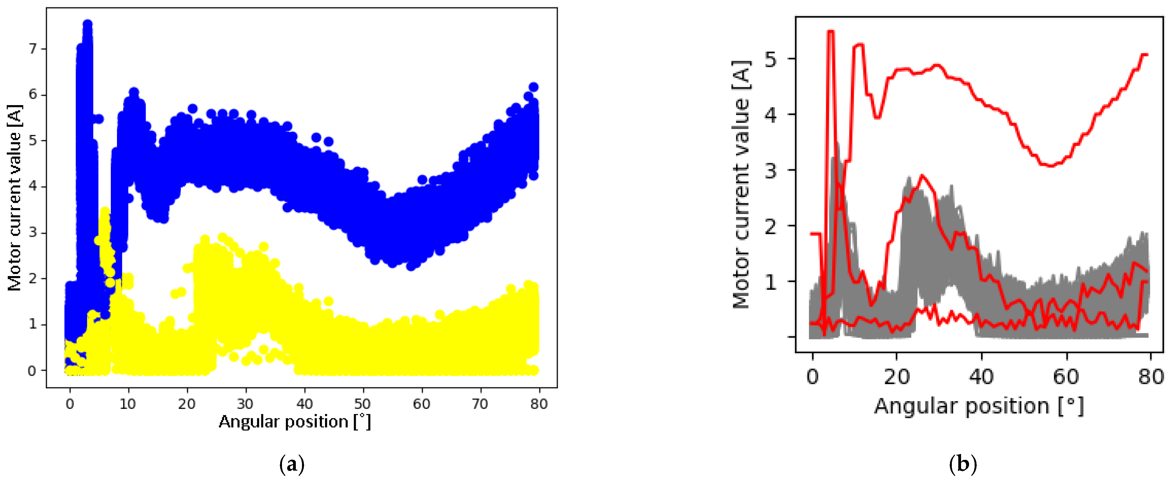
The first operation to be performed was to divide input data into two subgroups, that is, readouts indicating downward boom movement (lowering of the barrier boom) and readouts indicating upward boom movement (lifting of the barrier boom). Additionally, outliers also must be labelled based on expert knowledge. The dataset preparation process is depicted in Figure 4.

3.2. Data Scaling and Labelling

The second step was data scaling so that algorithms such as neural networks will not favour larger values over smaller ones (where both are equally significant). The scaler used in the application is a MinMax scaler (8) and its formula is as follows

$$i_{a,b}^S=\frac{i_{a,b}-\min \left(i_{1,b},i_{2,b}, \dots , i_{N,b}\right)}{\max \left(i_{1,b},i_{2,b}, \dots , i_{N,b}\right)-\min \left(i_{1,b},i_{2,b}, \dots , i_{N,b}\right)}$$

(8)

where:

• $i_{a,b}^S$ is an output scaled feature vector
• $i_{a,b}$ is an input feature vector.

3.3. Clustering Method

The vast majority of current waveforms (with regard to barrier machine systems) come with labelled data, each reading is marked with a flag denoting whether the boom is going up or down. Unfortunately, there are systems that do not provide such handy data; in these cases, the waveforms need to be labelled in order to apply the correct classifier in further analysis. To do so, there are numerous algorithms that can be applied such as k-nearest neighbours, Gaussian mixture models, DBSCAN or others (one of the clustering method, a self-organizing map is described further on in the paper). When the waveform is correctly labelled, anomalies can be analysed.

4. Outlier Detection

Anomalies were divided into two major subgroups—outliers [17] and novelties [18]. The first is based on the fact that there is a certain number of deviations among all the readouts in the training dataset. These algorithms find more populated regions and separate them from distant samples, which indicate anomalies. The other approach, novelty detection, takes only the unpolluted subset of data into account (for the sake of training) and focuses on detecting anomalies as samples not belonging to a pre-trained group. In the sub-sections below, we compare four highly different anomaly detection algorithms: local outlier factor, isolation forest, self-organizing map and autoencoder neural network.

Having prepared the data, the anomaly detection algorithms can be applied. The remaining steps to be taken include training the model and feeding unknown data into it to obtain a continuous probability score or a binary classification score. The whole data flow is shown in Figure 5.

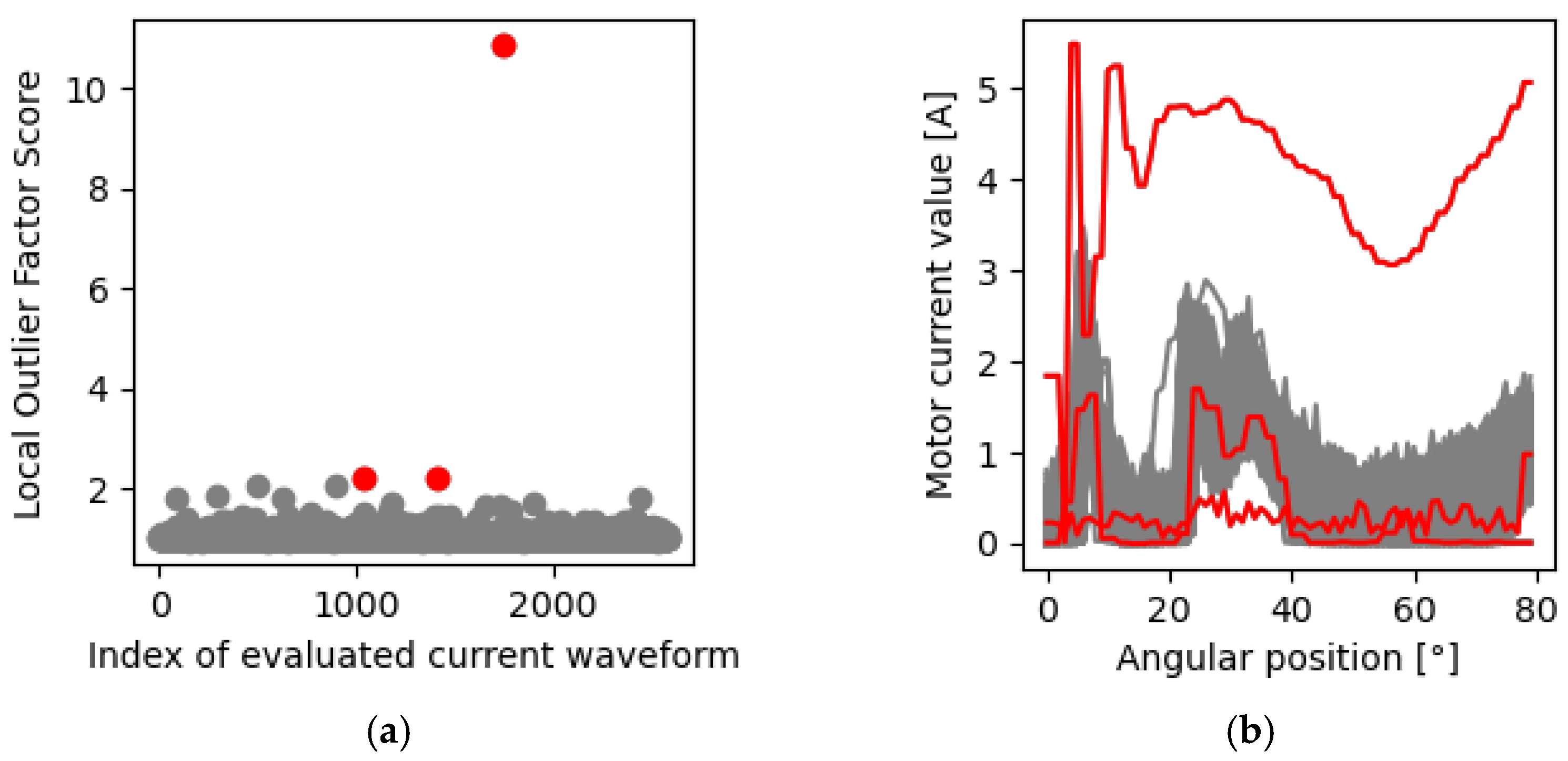
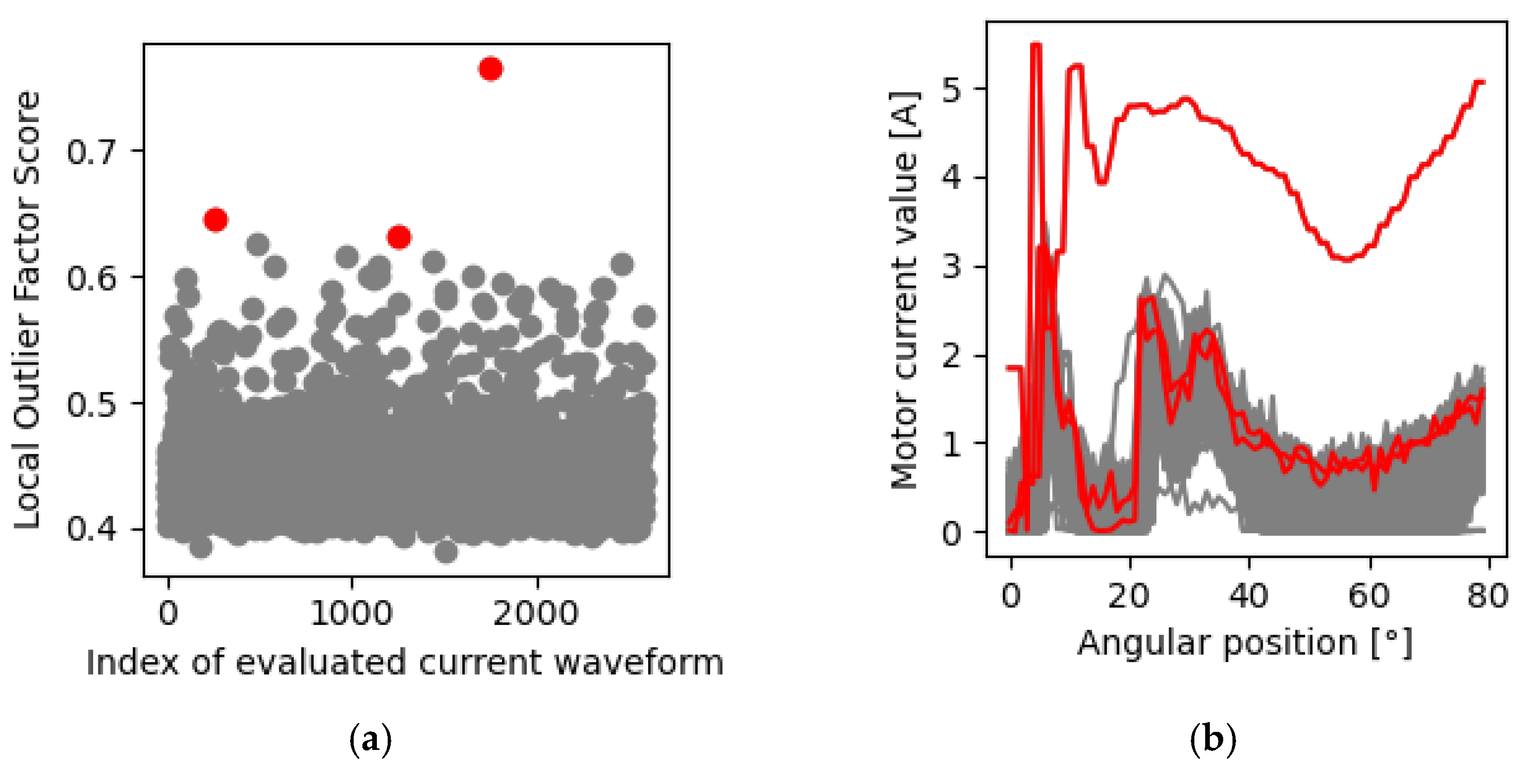
4.1. Local Outlier Factor (LOF)

One of the most popular approaches for outlier searching is LOF. The main idea behind this algorithm is to compare a sample’s local density with local densities of its k-nearest neighbours. The idea of reachability distance (RD) and local reachability density (LRD) derived from local density is represented by the Formulas (9, 10), presented below, and is directly used to calculate the LOF score (11).

$$R{D}_k\left(I_A,I_B\right)=\max \left(N{D}_k\left(I_B\right), d\left(I_A,I_B\right)\right)$$

(9)

$$LR{D}_k\left(I_A\right)=\frac{1}{\frac{{\sum }_{j\in N_k\left(I_A\right)}R{D}_k\left(I_A,j\right)}{\left|N_k\left(I_A\right)\right|}}$$

(10)

$$LO{F}_k\left(I_A\right)=\frac{{\sum }_{j\in N_k\left(I_A\right)}LR{D}_k\left(j\right)}{\left|N_k\left(I_A\right)\right|LR{D}_k\left(I_A\right)}$$

(11)

where:

• k-distance $N{D}_k\left(I_B\right)$ is defined as a distance between object $I_B$ to its k-th neighbour
• $N_k\left(I_A\right)$ denotes the set of k nearest neighbors for object $I_A$.

The bigger the local density, the more likely the sample is an outlier. Figure 6 shows the outcome of outlier detection for the three most anomalous readings with the number of neighbours equalling k = 20.

The local outlier factor algorithm managed to successfully classify two of the most anomalous waveforms, but incorrectly classified the remaining one (see Figure 4 for expert-chosen outliers).

4.2. Isolation Forest (iForest)

Isolation forest is widely known for its low computational complexity and its effectiveness on high-dimensional data. Unlike the majority of anomaly detection methods, iForests is based on actually isolating anomalies instead of profiling correct readings. Its operation is based on binary search trees and can be described as dividing hyperplane n-times for each sample (until a sufficient number of slices for distinguishing one particular object is achieved) and building forests on those sets of divisions. The less divisions each sample requires for its homogenous classification, the more likely it is an anomaly. The anomaly score for iForest is described by Formula (12) below.

$$IF\left(I_A,n\right)=2^{-\frac{E\left(h\left(I_A\right)\right)}{c\left(n\right)}},$$

(12)

where:

• $h\left(I_A\right)$ is the level of the branch for classifying observation $I_A$
• $c\left(n\right)$ is the average branch level
• n denotes the number of external nodes
• $E\left(h\left(I_A\right)\right)$ denotes the average value of $h\left(I_A\right)$ for all the isolation trees.

The first glance of this approach (training dataset) on the current waveforms of barrier machines (boom going down) is presented in Figure 7 below.

Isolation forest correctly classified the most outlying waveform, but incorrectly classified the other two.

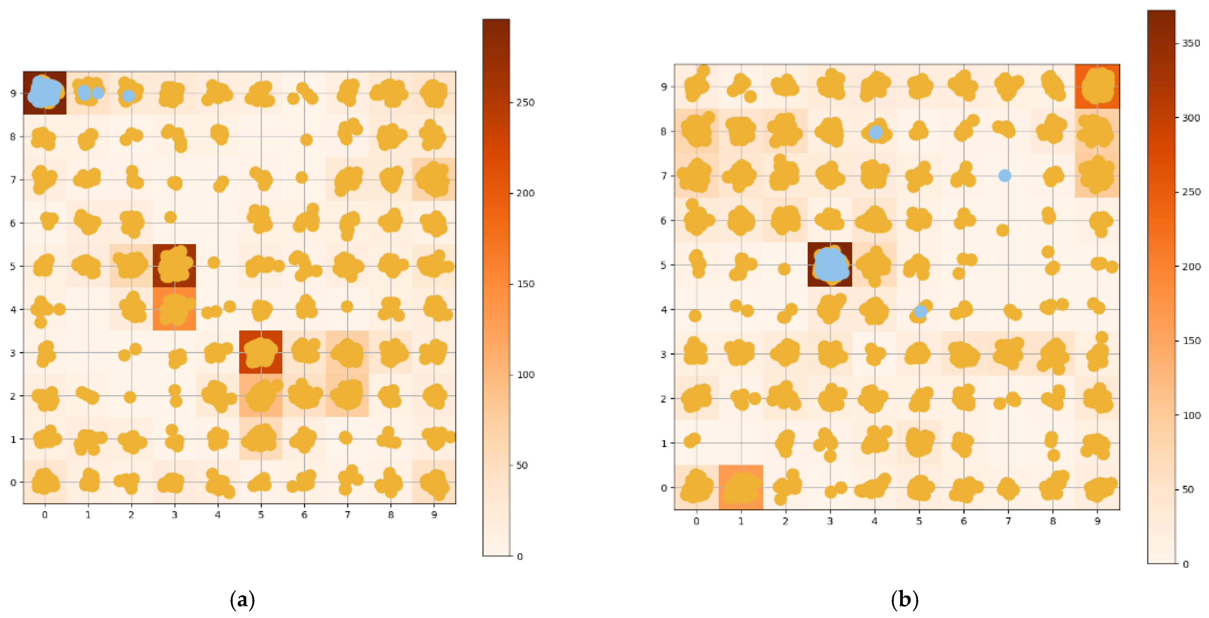
4.3. Self-Organizing Map (SOM)

Self-organizing maps are a great tool when it comes to computing two-dimensional (commonly) representations of input spaces and preserving their topology. As the algorithm progresses, the map becomes more and more like the population; the neurons start to cover the whole dataset in terms of (e.g., Euclidean) distance. As the algorithm progresses, the random n by m vector map is updated so that for each randomly picked input vector $I_{rand\_int\left(1,N\right)}$ from the J population of all current samples vectors $\left[I_{1 }, I_{1 }, \dots , I_N\right]$, its best matching unit (BMU) is found in the Korhonen map. This W unit and their closest neighbours are updated (Formula 13) with the learning rate η until all the iterations are finished.

$$W^{\prime }=W+\eta \left(I_{rand\_int\left(1,N\right)}-W\right)$$

(13)

This feature enables the use of SOM as an outlier detection algorithm. The readings that are placed in less populated regions may be considered anomalies while correct vectors tend to form larger clusters, as shown in Figure 8.

Although SOM turned out to be a perfect classifier (all the readings were clustered correctly into two subsets), the hypothesis on finding anomalies in less populated areas appeared to be incorrect, that is, contrary to expectations, outliers were assigned to bigger clusters. To get around this problem, the SOM algorithm was fed with clustered data (both subsets) and the outcome of this approach is presented in Figure 9.

Such a division of datasets caused another problem, as vectors in the same subgroup did not significantly differ from one another, the maps were almost equally covered by the samples, thereby disabling any further cauterization or outlier detection.

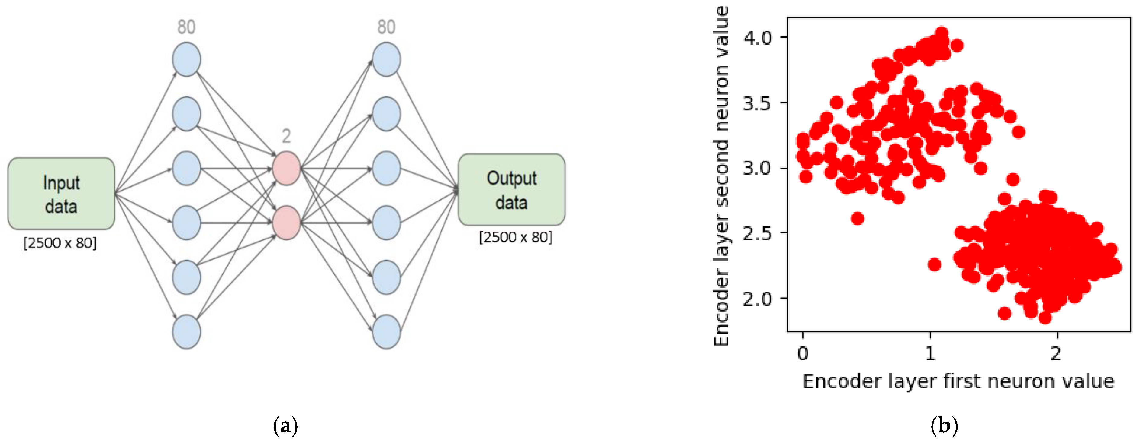
4.4. Autoencoder Neural Network

Neural networks are becoming increasingly popular as the computational capabilities of computers develop. They are widely used for image recognition, classification, regression and much more. Among all the back propagation neural network structures there are several subgroups, such as artificial neural networks [19], convolutional neural networks [20], recurrent neural networks [21], and others. For the purpose of anomaly detection, one network architecture, i.e., autoencoder [22,23] is widely used. It is based on the idea of compressing information into lower dimensionality and then decoding it. The network generalizes to the most common samples so the coding–decoding process is burdened with the most minor sample error, while outliers respectively cause a larger mismatch between input and output. 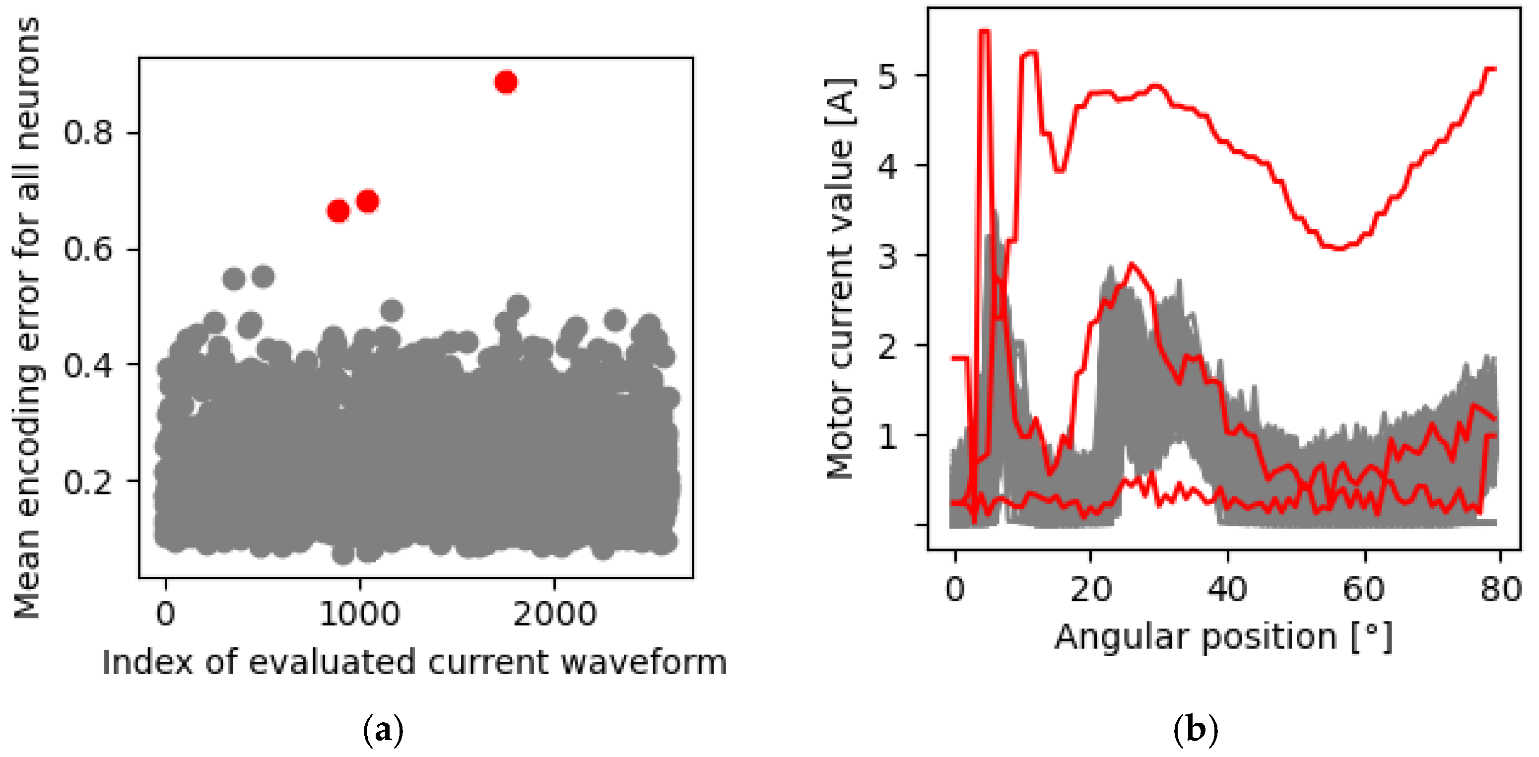The network shown in Figure 10 was created for the purpose of finding outliers in the delivered dataset.

Figure 11 shows the outcome of outlier detection for the autoencoder shown above in Figure 10, with an input layer size of 80, two encoding neurons, a decoding layer size of 80, rectified linear unit (ReLU) encoding activation function, sigmoid decoding activation function, 3000 training epochs and a batch size equal to 1.

5. Comparison of the Methods

For assessing the accuracy of each method, we used 50 supply current waveforms gathered from a real barrier machine and 43 waveform models from Section 2. The simulated faults included: boom hits a solid obstacle, e.g., a car (FSO_sim = 13 waveforms), gear wear at certain levels (FGF_sim = 10 waveforms), boom hits a flexible obstacle, e.g., a branch or an animal (FFO_sim = 10 waveforms), and supply current noises of different amplitude (FN_sim = 10 waveforms).

All of the proposed anomaly detection algorithms (LOF, iForest and autoencoder) were tested on these values.

Table 1. Confusion matrices for LOF, iForest and autoencoder.

LOF	Positive	Negative
Predicted Positive	TP: 315	FP: 61
Predicted Negative	FN: 85	TN: 339
iForest	Positive	Negative
Predicted Positive	291	42
Predicted Negative	109	358
Autoencoder	Positive	Negative
Predicted Positive	330	57
Predicted Negative	70	343

shows the confusion matrices which include the numerical values for true positive (TP), true negative (TN), false positive (FP) and false negative (FN) classifier hits.

Additionally, sensitivity, specificity and accuracy scores (14) are presented in

Table 2. Sensitivity and specificity scores for LOF, iForest, and Autoencoder.

Score	LOF	iForest	Autoencoder
Sensitivity	79%	73%	83%
Specificity	85%	90%	86%
Accuracy	82%	81%	84%

.

$$\begin{gathered} sensitivity=\frac{TP}{TP+FN} , \\ specificity=\frac{TN}{TN+FP} , \\ accuracy=\frac{TN+TP}{TN+TP+FN+FP} \end{gathered}$$

(14)

The data presented in Table 1 and Table 2 show the sensitivity and specificity scores of various classifiers optimized for reaching maximum accuracy. As can be seen, the autoencoder achieved the best result for accuracy of 84%. Nonetheless, local outlier factor performs surprisingly well for a method that uses only neighbourhood similarity metrics, obtaining a slightly worse score for both sensitivity and specificity. Isolation forest did far worse in regard to sensitivity compared to both autoencoder and LOF, but on the other hand it showed the best specificity (90%). Detailed information on the specific anomaly detection rate can be found in

Table 3. Anomaly detection rate for the proposed approaches.

Anomaly	Detection Rate
	LOF	iForest	Autoencoder
Severe gear damage	100%	93%	100%
Obstacle hit	47%	30%	68%
White noise	86%	92%	92%
Gear wear	82%	76%	82%
Non-anomalous waveforms classified correctly	85%	90%	86%

(scores obtained for the same models as used for creating Table 1 and Table 2).

When it comes to detecting anomalies using SOM (using the same data as for evaluating all the models listed above), 97.5% of total anomalies concerning closing the barrier machine were placed in the most populated cluster (the one that contains around 8% of all non-anomalous waveforms). For the barrier boom going up 97.6% of total anomalies concerning closing the barrier machine were grouped in the fourth most populated cluster (the one containing about 6% of all non-anomalous waveforms). Such an output completely disqualifies Kohonen maps from further use as the vast majority of anomalies are classified in the same manner as the most representative inliers.

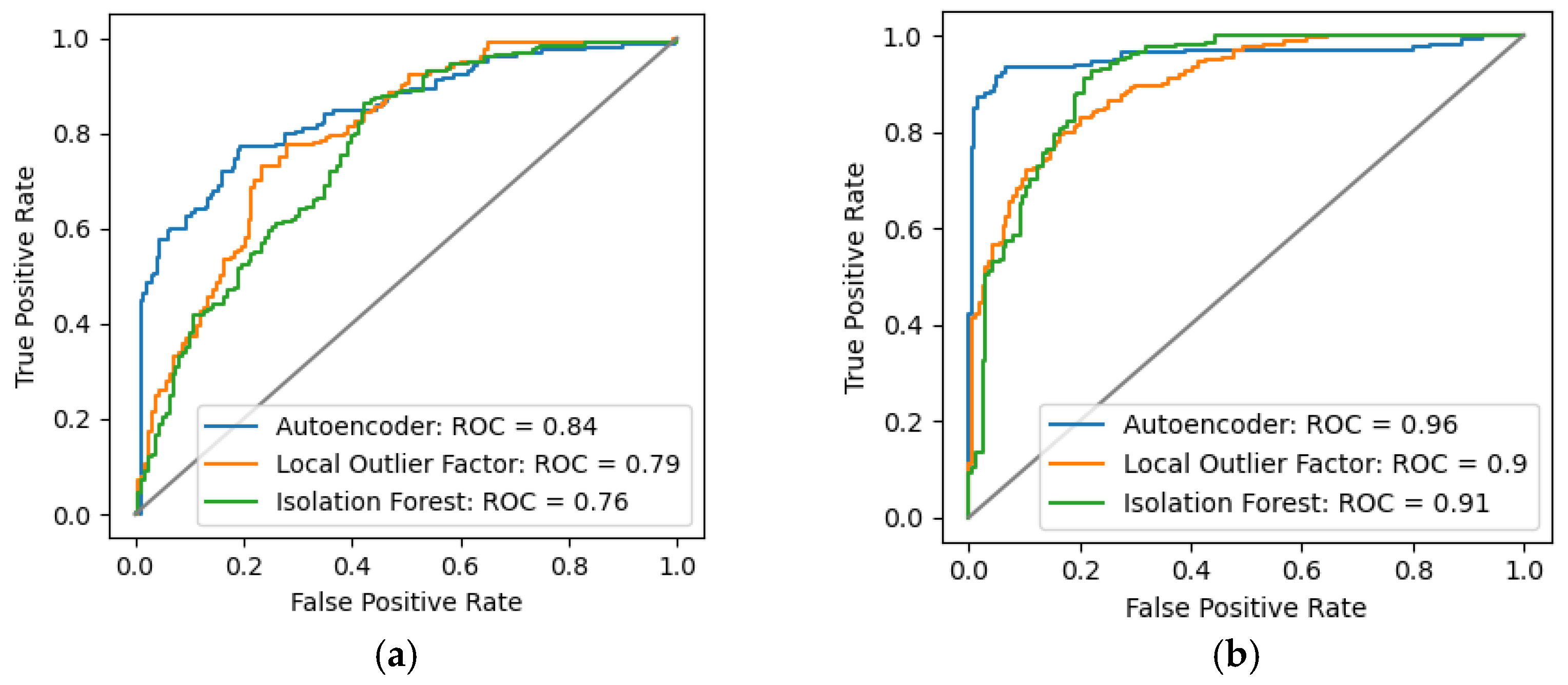
The sensitivity and specificity scores can both be increased at the expense of lowering the other (using the cut-off value settings). Such a feature plays an important role when taking into account, e.g., the cost of unnecessary relocations of service personnel—in this case the specificity score should be boosted (by raising the cut-off). On the other hand, when the barrier machine is placed in a dense traffic area, it is better to react to even false-positive alarms than to disregard even one real alarm indication (this is where the sensitivity score becomes important). However, we must remember to tune these settings with great caution. The ROC curve accurately represents the model’s performance in terms of tuning the cut-off values (Figure 12). The curve is defined as a function of the true positive rate vs. false positive rate values, the higher the area under the curve, the better a particular model performs. A comparison of the models proposed in this paper in terms of ROC curve visualization is presented below.

What needs to be kept in mind is the nature of a particular approach, e.g., autoencoders are the best when it comes to performance, but they are also the most computationally complex; it takes several times longer to train such a model than the LOF or forest. Moreover, heuristic methods such as autoencoder and iForest may provide different models for the same training dataset, so performing several experiments (besides optimizing hyperparameters) may be a good way to obtain a proper output. Such a step is not applicable to deterministic algorithms such as LOF, as the model will always remain constant if training is run on the same data.

6. Conclusions

This paper discusses a very important aspect of the automatic level crossing systems. Faultless performance of barrier machines has a significant impact on the safety and availability of railway systems. We introduced four fault models for the barrier machine and proposed a fault and anomaly detection procedure based on the current waveform measurements. All of the barrier machine models were based on real observations acquired at the test bench. Artificial intelligence-based algorithms were proposed to detect a predefined set of faults. Among the various methods, the autoencoder method seems to be the most suitable because it had the highest sensitivity score. This enables correct detection of the defined faults, i.e., a barrier machine boom hits a flexible obstacle (FFO), and the mechanical gearbox of the barrier machine is degraded. Repeated detection of such events should trigger earlier intervention by maintenance staff. All the presented methods proved to be effective in terms of detecting serious fault states when a barrier boom hits a solid obstacle (FSO) while rising or falling. The applied procedures with predefined faults provide new insights into a specific application—a barrier machine equipped with a boom.

The proposed approach may be applied for the purpose of dynamically developing preventive maintenance within the railway industry and may increase safety at level crossings. It is worth pointing out that this additional diagnostic functionality can be added to the railway system as an isolated block; the current measurement module and processing module can easily be galvanically separated from the existing circuits of the system. The output information can be merged with the existing stream of data observed and analysed by the maintenance staff. This approach ensures that the diagnostic part of the system will not have any impact on its safety. The other option is to directly incorporate the new functionality into existing control algorithms of the level crossing system. The resulting information indicating a detected anomaly shall be processed according to the existing or newly defined requirements. Because the broken barrier machine equally affects railway and road users, a highly reliable and cost-effective solution is needed to prevent faults, traffic disruption and assure public safety. Considering the impact of failure-free performance of barrier machines on safety, it is advisable and justifiable to continue the research on this issue.

The promising results encourage further analysis, which might include examining the possibility of detecting gusts of winds of a speed close to a defined maximum (especially in the case of barrier machine applications with long booms and skirts), as well as the verification and further improvement of the presented methods using real-life data.

References

- Liang, C.; Ghazel, M.; Cazier, O.; Bouillaut, L. Advanced Model-Based Risk Reasoning on Automatic Railway Level Crossings. Saf. Sci. 2020, 124, 104592. [Google Scholar] [CrossRef]
- Freeman, J.; McMaster, M.; Rakotonirainy, A. An Exploration into Younger and Older Pedestrians’ Risky Behaviours at Train Level Crossings. Safety 2015, 1, 16–27. [Google Scholar] [CrossRef]
- Kampczyk, A. An Innovative Approach to Surveying the Geometry of Visibility Triangles at Railway Level Crossings. Sensors 2020, 20, 6623. [Google Scholar] [CrossRef] [PubMed]
- PN-EN 50129:2019-01—Wersja Angielska. Available online: https://sklep.pkn.pl/pn-en-50129-2019-01e.html (accessed on 19 January 2021).
- Statystyki. Available online: https://www.bezpieczny-przejazd.pl/o-kampanii/statystyki/ (accessed on 8 January 2021).
- Jia, X.; Jin, C.; Buzza, M.; Di, Y.; Siegel, D.; Lee, J. A Deviation Based Assessment Methodology for Multiple Machine Health Patterns Classification and Fault Detection. Mech. Syst. Signal Process. 2018, 99, 244–261. [Google Scholar] [CrossRef]
- Oztemel, E.; Gursev, S. Literature Review of Industry 4.0 and Related Technologies. J. Intell. Manuf. 2020, 31, 127–182. [Google Scholar] [CrossRef]
- Ganesan, S.; David, P.W.; Balachandran, P.K.; Samithas, D. Intelligent Starting Current-Based Fault Identification of an Induction Motor Operating under Various Power Quality Issues. Energies 2021, 14, 304. [Google Scholar] [CrossRef]
- Lee, C.-Y.; Cheng, Y.-H. Motor Fault Detection Using Wavelet Transform and Improved PSO-BP Neural Network. Processes 2020, 8, 1322. [Google Scholar] [CrossRef]
- Azamfar, M.; Jia, X.; Pandhare, V.; Singh, J.; Davari, H.; Lee, J. Detection and Diagnosis of Bottle Capping Failures Based on Motor Current Signature Analysis. Procedia Manuf. 2019, 34, 840–846. [Google Scholar] [CrossRef]
- Grzechca, D.; Ziębiński, A.; Rybka, P. Enhanced Reliability of ADAS Sensors Based on the Observation of the Power Supply Current and Neural Network Application. In Computational Collective Intelligence; Nguyen, N.T., Papadopoulos, G.A., Jędrzejowicz, P., Trawiński, B., Vossen, G., Eds.; Lecture Notes in Computer Science; Springer International Publishing: Cham, Switzerland, 2017; Volume 10449, pp. 215–226. ISBN 978-3-319-67076-8. [Google Scholar]
- Kamat, P.; Sugandhi, R. Anomaly Detection for Predictive Maintenance in Industry 4.0—A Survey. E3S Web Conf. 2020, 170, 02007. [Google Scholar] [CrossRef]
- Chen, Z.; Xu, K.; Wei, J.; Dong, G. Voltage Fault Detection for Lithium-Ion Battery Pack Using Local Outlier Factor. Measurement 2019, 146, 544–556. [Google Scholar] [CrossRef]
- Cheng, Z.; Zou, C.; Dong, J. Outlier Detection Using Isolation Forest and Local Outlier Factor. In Proceedings of the Conference on Research in Adaptive and Convergent Systems, Chongqing, China, 24 September 2019; ACM: New York, NY, USA, 2019; pp. 161–168. [Google Scholar]
- Nguyen, T.-B.-T.; Liao, T.-L.; Vu, T.-A. Anomaly Detection Using One-Class SVM for Logs of Juniper Router Devices. In Industrial Networks and Intelligent Systems; Duong, T.Q., Vo, N.-S., Nguyen, L.K., Vien, Q.-T., Nguyen, V.-D., Eds.; Lecture Notes of the Institute for Computer Sciences, Social Informatics and Telecommunications Engineering; Springer International Publishing: Cham, Switzerland, 2019; Volume 293, pp. 302–312. ISBN 978-3-030-30148-4. [Google Scholar]
- Wang, C.; Wang, B.; Liu, H.; Qu, H. Anomaly Detection for Industrial Control System Based on Autoencoder Neural Network. Wirel. Commun. Mob. Comput. 2020, 2020, 1–10. [Google Scholar] [CrossRef]
- Hodge, V.J.; Austin, J. An Evaluation of Classification and Outlier Detection Algorithms. arXiv 2018, arXiv:180500811. [Google Scholar]
- Domingues, R.; Michiardi, P.; Barlet, J.; Filippone, M. A Comparative Evaluation of Novelty Detection Algorithms for Discrete Sequences. Artif. Intell. Rev. 2020, 53, 3787–3812. [Google Scholar] [CrossRef]
- Abiodun, O.I.; Jantan, A.; Omolara, A.E.; Dada, K.V.; Mohamed, N.A.; Arshad, H. State-of-the-Art in Artificial Neural Network Applications: A Survey. Heliyon 2018, 4, e00938. [Google Scholar] [CrossRef] [PubMed]
- Shamsaldin, A.; Fattah, P.; Rashid, T.; Al-Salihi, N. A Study of The Convolutional Neural Networks Applications. UKH J. Sci. Eng. 2019, 3, 31–40. [Google Scholar] [CrossRef]
- Yu, Y.; Si, X.; Hu, C.; Zhang, J. A Review of Recurrent Neural Networks: LSTM Cells and Network Architectures. Neural Comput. 2019, 31, 1235–1270. [Google Scholar] [CrossRef] [PubMed]
- Borghesi, A.; Bartolini, A.; Lombardi, M.; Milano, M.; Benini, L. Anomaly Detection Using Autoencoders in High Performance Computing Systems. Proc. AAAI Conf. Artif. Intell. 2019, 33, 9428–9433. [Google Scholar] [CrossRef]
- Nolle, T.; Luettgen, S.; Seeliger, A.; Mühlhäuser, M. Analyzing Business Process Anomalies Using Autoencoders. Mach. Learn. 2018, 107, 1875–1893. [Google Scholar] [CrossRef]
Figure 1.
Barrier machine of an automatic level crossing system.
Figure 2.
(a) Current waveforms when a barrier boom is moving down. Correct readings are marked in grey; anomalies in pink (boom has hit a solid obstacle), green (white noise), blue (gear fault), red (boom has hit a flexible obstacle); (b) Current waveforms when a barrier boom is going up. Correct readings are marked in grey; anomalies in pink (a serious damage), green (white noise), blue (gear fault), red (obstacle has been hit).
Figure 3.
Block diagram representing data pre-processing pipeline.
Figure 4.
(a) Current waveforms of all readouts divided into groups according to their status: closing of the barrier machine (yellow) and opening the barrier machine (blue); (b) Correct current readouts (grey) and outliers (red).
Figure 5.
Block diagram representing the data flow in the presented approach.
Figure 6.
(a) Local outlier factor on the whole training dataset (boom moving down); (b) Three most anomalous waveforms (red) among the whole training dataset (grey).
Figure 7.
(a) iForest raw scoring function on the whole training dataset (boom moving down); (b) Three most anomalous waveforms (red) among the whole training dataset (grey).
Figure 8.
(a) Distance map for the whole dataset; (b) SOM representation of barrier machine opening (yellow) and closing (blue) current waveforms.
Figure 9.
(a) SOM representation of barrier machine opening current waveforms; (b) SOM representation of barrier machine closing current waveforms.
Figure 10.
(a) Visual representation of the autoencoder’s architecture; (b) Visualization of encoding neurons for the training dataset.
Figure 11.
(a) Average mean squared error of autoencoder’s decoding for each waveform in the population; (b) Three most anomalous waveforms (red) selected with autoencoder from the population (grey).
Figure 12.
(a) ROC curves of used methods for model concerning the boom moving down (b) ROC curves of used methods for model concerning the boom moving up.