Article

Economic Development, CO2 Emissions and Energy Use Nexus-Evidence from the Danube Region Countries

1
Department of Mathematical Methods and Managerial Informatics, Faculty of Management, University of Prešov, 080 01 Prešov, Slovakia
2
Department of Environmental Management, Faculty of Management, University of Prešov, 080 01 Prešov, Slovakia
*
Author to whom correspondence should be addressed.
Energies 2021, 14(11), 3165; https://doi.org/10.3390/en14113165
Submission received: 30 April 2021 / Revised: 20 May 2021 / Accepted: 24 May 2021 / Published: 28 May 2021
(This article belongs to the Special Issue Affordable Clean Energy: Methodological Aspects of Its Evaluation)

Abstract

:
The aim of this study is to examine the empirical cointegration, long-run and short-run dynamics and causal relationships between carbon emissions, energy consumption and economic growth in 14 Danube region countries over the period of 1990–2019. The autoregressive distributed lag (ARDL) bounds testing methodology was applied for each of the examined variables as a dependent variable. Limited by the length of the time series, we excluded two countries from the analysis and obtained valid results for the others for 26 of 36 ARDL models. The ARDL bounds reliably confirmed long-run cointegration between carbon emissions, energy consumption and economic growth in Austria, Czechia, Slovakia, and Slovenia. Economic growth and energy consumption have a significant impact on carbon emissions in the long-run in all of these four countries; in the short-run, the impact of economic growth is significant in Austria. Likewise, when examining cointegration between energy consumption, carbon emissions, and economic growth in the short-run, a significant contribution of CO2 emissions on energy consumptions for seven countries was found as a result of nine valid models. The results contribute to the information base essential for making responsible and informed decisions by policymakers and other stakeholders in individual countries. Moreover, they can serve as a platform for mutual cooperation and cohesion among countries in this region.

1. Introduction

Energy has played an important role in human development and is closely linked to all human activities. Although fundamental to economic growth, energy production and consumption (among other factors, such as population growth and deforestation) is also responsible for many negative effects on the environment and human well-being, such as climate change and global temperature rise caused by increased greenhouse gas emissions into the atmosphere. As most energy systems are based on fossil fuels, high energy consumption also leads to an unsustainable reduction in non-renewable fossil fuel resources. That is the reason why these issues have emerged as central topics in global discussions on the transition to a green economy [1,2,3]. The fundamental importance of these issues to sustainable and prosperous development is likewise reflected in the EU’s medium- and long-term planning.
Energy and resource efficiency, as well as climate protection is one of the top strategic priorities of the EU supported by a number of long-term objectives. Present initiatives of the EU such as the European Green Deal [4]—the EU’s instrument for achieving its ambitious goal of carbon neutrality is a prominent example. These initiatives are complemented by policies addressing specific pressures and sectors, such as the adoption of an EU strategy for the integration of the energy system [5] and an EU hydrogen strategy [6] to support decarbonisation and climate neutrality of the EU by 2050.
In order to increase green growth and strengthen cooperation at a macro-regional level, the European Union established the EU Strategy for the Danube Region (EUSDR) with eleven priority areas, among them is one dedicated to energy. The Danube Region is characterised by a divergent group of 14 countries (9 of them are EU member states, 5 are non-EU countries) concerning the level of their integration and the preconditions in geographic, economic, cultural, and socio-demographic terms [7,8].
The Danube region is facing a number of challenges, including environmental and energy issues (environmental degradation, energy dependence, insufficient energy infrastructure), as well as discrepancies in socio-economic development. As Borowsky [9] states, the energy market, including the Danube region, experiences significant changes in deregulation, competitiveness and efficiency. The region connects countries that are not only highly heterogeneous in terms of their economic performance but also countries with ultimately different energy systems, relying on uncoordinated national support schemes and different technologies. Energy prices are high in the Danube Region compared to other parts of Europe, mostly due to fragmented markets and overreliance on a limited number of energy suppliers [10]. Primary energy is mainly imported, its transport is costly, the markets are fragmented, and energy infrastructures are not well interconnected. In addition, the Danube Region is specifically vulnerable regarding the security of supply, as was demonstrated in January 2009 during the Russia–Ukraine gas crisis, when gas supplies were cut. Energy production and consumption are also significant sources of environmental pollution. A greater diversity of supply at the national level through interconnections, a growing share of renewable energy sources and the establishment of a genuine regional market may significantly increase energy security [9,11,12].
The Danube Region strategy addresses energy-related issues in several aspects. The strategy devotes one of the Priority areas (PA) entirely to energy: PA2-sustainable energy, which strives to encourage sustainable energy systems in the region. However, energy is also closely related to PA8-Competitiveness of enterprises, of which the objective is to improve the technical knowledge and implementation level of environmental technologies through the presentation of the latest know-how in the area, including technologies for the generation of energy from renewable sources.
Moreover, the strategy pillar devoted to protecting the environment also touches on energy issues, as the energy sector is one of the main sources of air pollution in the region.
The strategy presents a platform to ensure the security of supply, to create a functioning energy market and to realise economies of scale in investments. Regarding energy efficiency and renewable energy, there is a significant potential still untapped. Investment in energy efficiency measures and the support of energy from renewables (also from small and private producers) using the potential of the region would be beneficial for the whole region and its inhabitants.
Concerning energy infrastructure, the aim is to coordinate the long-term energy policies as well as the national investment strategies to create win-win situations for all countries. Contributing to the achievement of Agenda 2030’s sustainable development goals and the climate goals specified in the Paris Agreement, to which the European Union is strongly committed, will require careful strategic energy management, efficient use of energy resources, and support for research and technological innovations at both regional and national levels as well as strong cooperation between countries.
The monitoring and measuring of a country’s or region’s state of development and assessing its progress towards sustainable energy and climate goals while maintaining economic development plays an important role. Such outputs may foster responsible and informed decision-making and the development or modification of strategies and policies towards sustainability [13].
This article discusses the links between energy consumption, CO2 emissions and the economic growth of the Danube region countries in the period 1990–2019. To assess the relationship between these three variables, the autoregressive distributed lag (ARDL) method was applied.
In our study, we determine the following research hypotheses:
Hypotheses 1 (H1):
We assume that in most countries of the examined region, a long-run relationship from GDP to CO2 emissions will be demonstrated.
Hypotheses 2 (H2):
We assume that in most countries of the examined region, a long-run relationship from energy consumption to CO2 emissions will be demonstrated.
Hypotheses 3 (H3):
We assume that there will also be countries within the Danube region for which there will be no long-term relationship between the variables GDP, energy consumption and CO2 emissions.
The paper is organised as follows. First, the previous empirical research initiatives are reviewed, focused on assessing the relationship between economic growth, energy consumption, and CO2 emissions production. In Section 2 we outline the research methods and data used. The third section presents the results of the analysis, followed by the fourth section discussing the results of the research. The last part of the article summarises the results, points out the limits of the research and suggests the possibilities of practical implications of the results.

2. The Literature Background

The dilemma of promoting economic growth while attempting to reduce adverse environmental impacts and increase material and energy efficiency poses an unprecedented challenge, as well as the opportunity for society. Most of the world’s economies are looking for ways to support economic development without compromising the environment and the resources it provides.
For this purpose, several concepts have been developed, including de-materialisation, delinking, decoupling, decomposition and eco-efficiency. The basic idea of these concepts is to “get more out of less”, i.e., use material and energy more efficiently or reduce the quantity of material to produce the same economic value. The environmental impact remains the same or even decreases while the economy grows or is stabilised (e.g., [11,12,13].
Within environmental research, these approaches have been applied to several areas, e.g., de Bruyn et al. [14], Heiskanen and Jalas [15] and Vehmas, Luukkanen and Kaivooja [16] referred to “dematerialisation” as the delinking of economic activity from its material base. “Decarbonisation” refers to a decreasing energy intensity of economic activities, determined by CO2 emissions per GDP unit [17].
Within the current environmental research, these approaches have been applied in several areas and sectors, e.g., the decoupling of resource productivity from the economic growth [18], the decoupling of energy-related GHG emissions from economic growth [19], the decoupling of the economic growth from the environmental impacts due to EU-28 consumption [20] and decoupling the relationship between land-use intensity and the natural environment [21]. In the transport sector, Finel and Tapio [22] and Tapio [23] conducted a decoupling analysis of GDP from traffic volume and carbon dioxide emissions from transport, and Ru et al. [24] focused on the decoupling of CO2 emissions per capita from income per capita in developed countries. More recent studies in this area were performed by Jiang et al. [25], Zhang et al. [26], Wang et al. [27], etc. For example, Zhang and Ke [28] assessed the sustainability of China’s forestry development, where they conducted a macroanalysis of the linkages between forest resources, the number of employees, and economic development in key state-owned forest areas.
These methods found a wide application, especially in the energy sector. Balcilar et al. [29] distinguish three research strands of econometric models applied in the assessing interaction between environmental degradation, energy consumption and economic growth.
(1) The energy-growth nexus is emphasising the relationship between economic growth and energy consumption without taking into account the environmental quality of economic development. The cointegration of the two variables has been the subject of several studies, e.g., Apergis and Payne [30,31] reviewed the nexus between electricity and income, as well as the nexus between energy consumption and impact. Ozturk et al. [32] investigated the energy-income nexus of 51 countries covering the period 1971–2005. Their results reveal the existence of un-directional causality that runs from energy use to income level, and the existence of bidirectional causality supported the conservation and the feedback hypothesis. More recently, Fan et al. [33] use the log-mean Divisia index and Tapio decoupling index to analyse the decoupling degree and driving factors of energy consumption and economic development in the Qinghai–Tibet Plateau. Omri [34] reviewed the literature on the nexus between economic growth and four types of energy consumption: total energy consumption, electricity consumption, nuclear energy consumption and the consumption of renewable energy sources. A worldwide perspective was gained by Kan et al. [35], who assessed the decoupling states of GDP and energy use for eight typical economies during 2000–2011. The relationship between economic growth and various energy sources has been scrutinised by Vural [36] for renewable and non-renewable sources, by Ozturk and Al-Mulali [37] for natural gas consumption and by Ozcan and Ari [38] for nuclear energy consumption.
(2) The CO2-growth nexus has been explored in studies by Shahbaz et al. [39], who investigated the economic development–carbon emissions nexus for the G7 countries from the long-term perspective. Zhou et al. [40] performed a comparative analysis of the relationship and influencing factors between economic growth and industrial energy-related carbon emissions in China. The mutual relation between energy intensity and CO2 emissions was scrutinised by Naminse and Zhuang [41], who concluded that heavy reliance on coal consumption is possibly a dominant cause for the increase in carbon dioxide emissions in China. In the context of the EU member states, Chovancová and Vavrek [42] performed a spatial analysis of the resource and impact decoupling with a focus on energy consumption, where they assessed relations among energy-related emissions, energy consumption and the mitigation effect of renewable energy sources. Chovancová and Tej [19] used decoupling analysis in assessing the relationship between energy-related GHG emissions and economic growth of the energy sector in V4 countries. The differences in the residential energy-related CO2 emissions between urban and rural regions were assessed by Yang et al. [43] using the log-mean Divisia index and the Tapio decoupling model. Similarly, the combination of the two methods was used by Sadorsky [44] to study how energy-related CO2 emissions and their driving factors after the financial crisis compared to the period before the financial crisis, comparing the results of 19 major countries (G19), which form the core of the G20. The relationship between economic growth and environmental pollution has also been well documented in the literature of the environmental Kuznets curve (EKC). The EKC hypothesis postulates that when a certain level of wealth, income and consumption is reached, the individual indicators of environmental quality (air pollution, water pollution, deforestation) improve with continued growth. The EKC curve capturing this development is ideally in the shape of an inverted letter “U”. The concept of EKC in the field of energy efficiency has been applied in works by Turner and Hanley [45]; Dogan and Turkekul [46]; Balado-Naves et al. [47], etc.
(3) The energy-CO2-growth nexus combines both approaches to investigate three-way linkages among CO2 emissions, energy consumption and economic growth. The dynamic causal relationship between these three variables was examined by Ang [48], whose empirical results for France over the period 1960–2000 suggest that more energy use results in more CO2 emissions and CO2 emissions and output have a quadratic relationship in the long-run. In their thorough literature survey, Tiba and Omri [49] analysed the results of more than 100 scientific papers on the energy-environment-economic nexus. More recently, Zhang et al. [50] focused their scientific interest in the economy-carbon-energy nexus on 50 typical developing countries. The results of their study reveal the long-run equilibrium between carbon emissions and economic-energy variables. However, the regression results illustrate that features of the inverted U-shaped curve of EKC theory appear only in 7 countries. In the majority of developing countries, energy consumption poses a positive impact on carbon emissions.
In recent years, studies have begun to appear that add other factors to the basic trio of economic, environmental and energy indicators. Several studies examine the impact of urbanisation on economic growth, energy consumption and emissions; for example, Odugbesan and Rjoub [51] examined the causality between economic growth, energy consumption, CO2 emissions and urbanisation in MINT countries and confirmed a long-term relationship running from economic growth, energy consumption and CO2 emissions to urbanisation in all four surveyed countries. On the other hand, the study by Raggad [52] brings evidence that urbanisation has a negative and significant impact on CO2 emissions in Saudi Arabia; however, the relationship between economic growth and air pollution was positive in both the short and the long-run. The impact of urbanisation, together with trade openness and financial development on the energy-economy-emissions nexus, were analysed by Farhani and Ozturk [53]. Based on their findings, the positive financial development of Tunisia took place at the expense of increasing the levels of CO2 emissions.
Most of the research on the relationship between economic growth and energy-related environmental issues are based at the local, national or global scales. However, to the best of our knowledge, no previous study was performed for Danube region countries. To narrow this gap, the present study focuses on Danube region countries to analyse the economy-energy-emissions nexus in this cluster of countries. Moreover, the region consists of a heterogeneous group of countries, including long-term EU members as well as newcomers and non-EU members. Comparing their developments in economic growth, energy consumption, and CO2 emissions can be beneficial for strengthening cooperation and the promotion of cohesion among countries.

3. Materials and Methods

3.1. Data

The paper examines the relationship between economic growth (GDP per capita), energy consumption per capita and CO2 emission per capita for 14 Danube region countries. Out of the fourteen countries belonging to this cluster, we included only 12 countries in the analysis due to the data unavailability and short time series in the case of Moldova and Montenegro.
Time series vary from country to country. In the case of the Member States and Ukraine, we analysed the time series 1990–2019, but due to the unavailability of data for the countries outside the EU, these time series are shorter. In the case of Moldova and Montenegro, the time series were too short (Montenegro GDP per capita n = 20; Moldova energy consumption n = 11), and so, these countries were excluded from the analysis. In the case of Bosnia and Herzegovina, Serbia and Croatia, some tests could not be performed (failed), and the results of these 3 countries, although models were made, have a validity problem that could not be eliminated. The World Bank’s databases (GDP per capita in constant 2010 USD); BP Statistical Review of World Energy (energy consumption per capita in kWh) and the Global Carbon Project (CO2 per capita in tons) were used as data sources. Dataset is available in Supplementary Materials Section.
The descriptive statistics are presented in Table 1 where the number of observations (N), mean, minimum and maximum values and standard deviation is calculated for each country. The software tool Stata 15.1 was used for data processing and statistical analysis.
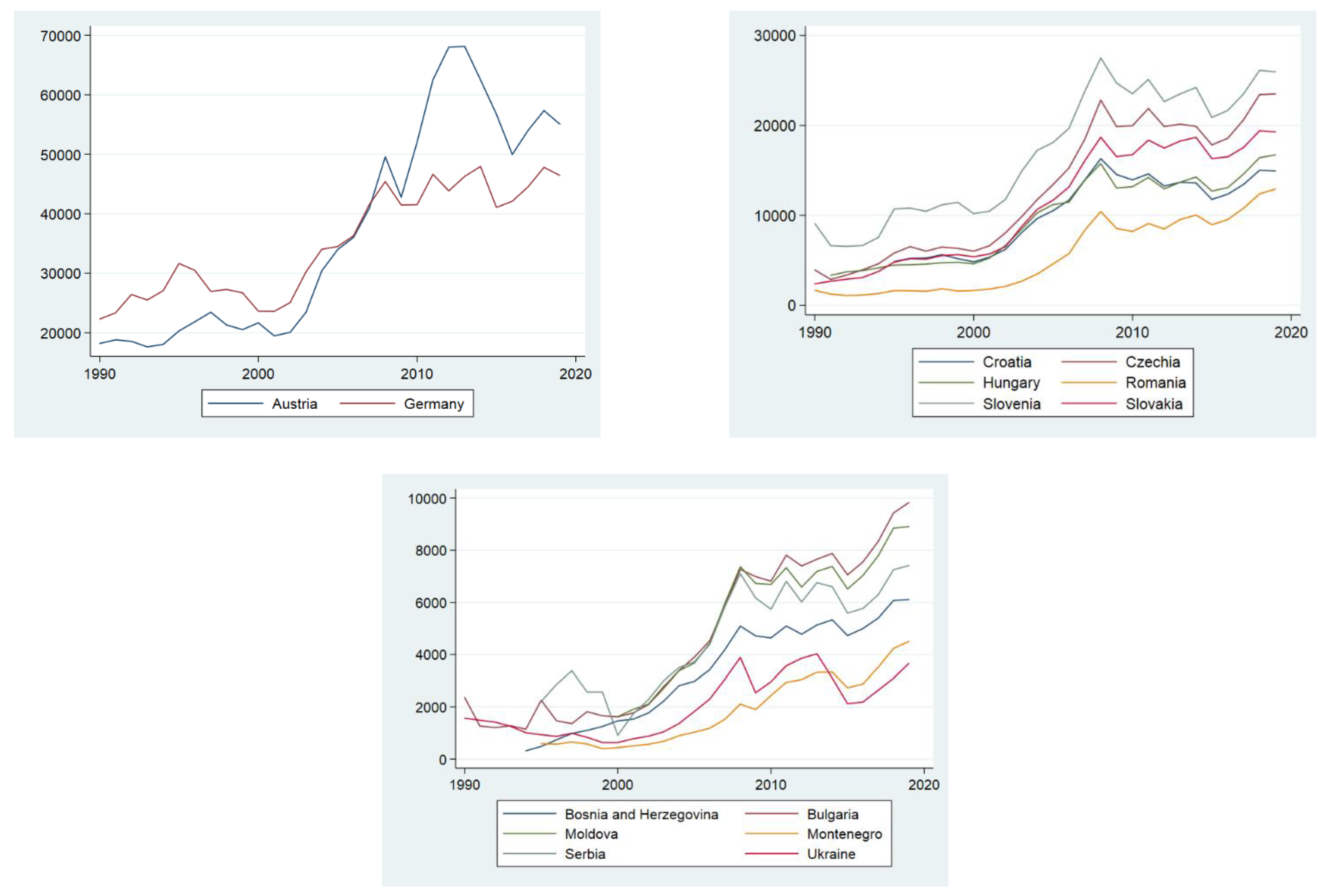
The time plot of carbon emissions per capita, energy consumption per capita and GDP per capita is presented in Figure 1.
The Czech Republic and Germany were the largest producers of CO2 emissions per capita in the surveyed group of countries. We recorded the lowest volume of carbon emissions in Moldova (Figure 1a). The Czech Republic, Austria and Germany are leaders in energy consumption per capita. In Moldova, energy consumption per capita was at its lowest level.
GDP per capita varies significantly among Danube region countries. Austria and Germany have the highest GDP per capita; on the opposite side of the spectrum are non-EU countries: Ukraine, Moldova, Bosnia and Herzegovina and Serbia.
In some countries, we observe significant differences in the development of individual variables, which was reflected in the high value of standard deviation. An example is Austria, where the GDP grew significantly during the period under review, which can be attributed to a highly developed industry and international tourism.
The opposite case is Ukraine, where we can observe a significant drop in all monitored variables, which probably corresponds to the country’s poor economic situation associated with the ongoing armed conflict.

3.2. Methodology

The theoretical and empirical literature signifies that economic growth, CO2 emissions and energy consumption are bound together. We work with such data from fourteen countries. In line with Odugbesan and Rjoub [51], economic growth and energy consumption are utilised in natural logarithm form. We use the abbreviations LGDPt, CO2t and LECt to denote their values at time t.
This research utilises the unit root test of Dickey and Fuller [54], the stationarity test of Kwiatkowski et al. [55] and the bound test for cointegration of Pesaran et al. [56], which is extended by the critical values and approximate p-values of Kripfganz and Schneider [57].
Some time series are bound together due to equilibrium forces despite the fact that the individual time series might move significantly. We focus on three such series, LGDPt, CO2t and LECt. The methodology to determine this long-term impact and significance of considered variables uses an autoregressive distributed lag (ARDL) modelling approach, widely developed by Pesaran and Shin [58] and Pesaran et al. [56], which allows establishing whether there is cointegration between the variables, even if they are of a different order. Due to the efficient estimation of model coefficients, using model selection criteria, such as the Akaike or Schwarz information criterion, obtains the optimal lag order. However, for testing purposes, it is essential that the error term does not contain a serial correlation. If a conclusion is drawn from the test, a more parsimonious model can be estimated [57].
An additional advantage of its estimation is that it allows obtaining unbiased and efficient parameters when the presence of endogeneity and serial correlation problems is suspected. In addition, it is more appropriate for estimating short and long term on small samples, which is also our case.
The augmented Dickey–Fuller (ADF) test was used as the first step for the stationarity test to ensure that none of the series used in this study is I (2).
To find a cointegration relationship between economic growth, CO2 emissions, and energy consumption, the employed ARDL (p, q1, q2) model can be expressed as follows:
y t = c 0 + i = 1 p ϕ i y t i + i = 0 q 1 β 1 , i x 1 , t i + i = 0 q 2 β 2 , i x 2 , t i + u t
where p 1 ,   q 1 0 ,   q 2 0 are optimal lag orders for the dependent variable y and 2 independent variables x1 and x2; ϕ and β are coefficients; c0 is a constant; ut is the error term. Independent variables have to be I (0) or I (1) or cointegrated. For each of the considered countries, we estimate three ARDL models for each of the three variables LGDPt, CO2t, and LECt in the position of the explained variable.
Error correction representation of the ARDL model serves for testing the cointegrating relationship between variables. A bounds testing procedure allows us to find out this relationship, regardless if the variables are integrated of the order zero or one. In this way, if the value calculated for the F-statistic is above the critical value of the upper limit, the null hypothesis of no cointegration is rejected, and the existence of a long-term relationship is concluded. On the contrary, if the F-statistic is below the critical value of the lower limit, it implies the absence of cointegration [56].
If the cointegration relationship is confirmed, the model can be represented by an error correction form [55]. The model can be written as follows:
Δ y t = c 0 α ( y t 1 θ 1 x 1 , t θ 2 x 2 , t ) + i = 1 p 1 ψ i Δ y t i + i = 0 q 1 1 γ 1 , i Δ x 1 , t i + i = 0 q 2 1 γ 2 , i Δ x 2 , t i + u t
where α is the speed adjustment parameter; θ-s is the long-run parameter, ψ-s and γ-s are short-run parameters. To confirm the long-term relationship, parameter α is expected to be negative and statistically significant. Likewise, to ensure the validity of the results of the cointegration test, the tests of heteroscedasticity, autocorrelation and normality of the residuals are applied. In line with Odugbesan and Rjoub [51], to test the serial correlation, we also used the Breusch–Godfrey serial correlation LM (lagrange multiplier) test. In order to test the heteroskedasticity, we applied the Breusch–Pagan–Godfrey test. For testing the normality of residuals, the SW test was used. Finally, as Pesaran et al. [56] recommend, the cumulative sum of recursive residuals (CUSUM) should be employed to determine the stability of ARDL model.

4. Results and Discussion

4.1. Results for Unit Root Test

To avoid an unpredictable result in our time series analysis, it is necessary to use a root unit test to determine the stationary nature of our data set [51]. Table 2 shows the augmented Dickey–Fuller unit-root test (ADF) analysis applied on the level and on the first difference. The time series of the GDP of Bosnia and Herzegovina is stationary already at the level. In the case of the other countries, all of the GDP variables have a unit root at the level and are stationary after the first differences. In the case of the variable CO2, all countries are stationary at the first difference, and there are five countries that are already stationary at the level, Bulgaria, Moldova, Romania, Slovakia and Ukraine. Bulgaria and Moldova are stationary at the level also in the variable energy consumption and in addition to them, Montenegro and Romania. It should be recalled here that the time series of countries Moldova and Montenegro was too short to allow further analysis. As for the first difference, all countries are also stationary in the variable CO2. Hence, a mix of order is corroborated, but ARDL cointegration is efficient in this case due to the bound testing. Results revealed that none of the variables used in the analysis is integrated in I (2), in order to ensure the assumptions of ARDL [56].
Another test to verify the stationarity of the considered time series was the KPSS test of Kwiatkowski et al. [55], using two added parameters according to Hobijn et al. (1998) due to a small sample. According to Baum [59], the author of KPSS procedure in the software Stata, the KPSS test has the more “natural” null hypothesis of stationarity (I (0)), where a rejection indicates non-stationarity (I (1) or I (d)). The KPSS test may be used to confirm the findings of an ADF test. If the result of these two tests is the same, it is convincing evidence of stationarity or non-stationarity. Hobijn et al. [60] state, “our Monte Carlo simulations show that the best small sample results of the test in case the process exhibits a high degree of persistence are obtained using both the automatic bandwidth selection procedure and the Quadratic Spectral kernel.”
The numerically presented result of the ADF test in Table 2 is supplemented by a bold indication in case of the same result also in the KPSS test with parameters according to Hobijn et al. [60]. It is clear from the table that the KPSS test evaluated the considered time series as stationary more often than the ADF test. Due to the further application of the ARDL test, the first difference is more important to us than the level. Here, in five cases (if we no longer consider Moldovia and Montenegro, which are not further analysed), the opposite result occurred. At the obvious significance level of 0.05, H0 stationarity in the KPSS test is rejected. However, if we consider the significance level of 0.01, H0 is confirmed, and we can conclude in five disputed cases that time series is stationary, as it has been shown in the ADF test. Therefore, no series is I (2).

4.2. Results for ARDL Bound Testing for Cointegration

Table 3 carries the results of the bound test showing F-values and the lower and upper critical F-values of Kripfganz & Schneider [57] at 5%.
The result for Austria and the same for Czechia, Slovakia and Ukraine, when CO2 is the dependent variable, shows that there is cointegration among CO2, economic growth and energy use. This indicates the occurrence of a long-run relationship among the investigated variables. It implies, there is a need to estimate the error correction model to determine the speed of adjustment in case of shock. In the case of GDP as well as energy consumption as the dependent variables, the result from the ARDL bounds test for cointegration indicates that there is no cointegration. Therefore, only ARDL (short-run model) was estimated.
In the case of Slovenia, two of the variables indicates cointegration when they are used as the dependent variable, CO2 and energy consumption. In that case, the error correction model was performed for these two models to reveal whether the long-run relationship is significant and to determine the speed of adjustment.
However, the bound test could not verify cointegration in four countries, Bulgaria, Germany, Hungary and Romania. Therefore, in these countries, only the ARDL (short-run model) was estimated for each of the three variables GDP, CO2 and energy consumption used as a dependent variable.
As for Croatia, the result from the bounds test reveals a cointegration when GDP and CO2 are the dependent variables, while in the case of energy consumption, the bound test failed due to the small number of data. Based on the experience and significance of the speed-of-adjustment coefficient and LR coefficients, we decided to use the error correction model here as well.
The same problem occurred with Serbia and Bosnia and Herzegovina. In Serbia, only in the case of the dependent variable energy consumption, the selection of the error correction model was verified by a bound test. Based on experience, we also opted for the error correction model for CO2, but the insignificant results of the error correction model for GDP directed us to the ARDL (short-run) model.
Finally, in Bosnia and Herzegovina, a bound test failed for each of the three variables (GDP, CO2 and energy consumption) used as a dependent variable. Due to the significance of the speed-of-adjustment coefficient and LR coefficients, we decided to apply the error correction model in all three cases.

4.3. Estimates for Causal Relationship

On the variables that contribute to the economic growth in the Danube region countries, the results depicted in Table 4 and Table 5 reveal that although in two countries, Bosnia and Herzegovina and Croatia, CO2 emissions and energy consumption have a long-run relationship with economic growth, the significance of the causality in Croatia could not be established. In addition, the model for Croatia is not valid due to the problem with the normality of random errors. Other tested models did not solve the problem either. The ECT coefficient of the stable long-run relationship for Bosnia and Herzegovina is −0.38 and significant at 0.05. Therefore, this implies that the economic growth converges to the long-run equilibrium by 38% in one period with the speed adjustment via the channel of energy consumption and CO2 emissions [61].
Moreover, the results shown in Table 6 and Table 5 reveal that there is also short-run causality running from energy consumption to economic growth in both Bosnia and Herzegovina and Croatia, whereas CO2 emissions have short-run causality to economic growth only in Croatia.
Table 6 reveals that there is also short-run causality running from CO2 emissions to GDP in Czechia, Germany, Romania, Slovakia, Slovenia and Ukraine, and short-run causality running from energy consumption to GDP in Germany, Romania and Slovakia, taking into consideration only valid short-run models.
Given the long-run relationship between carbon emissions, economic growth and energy consumption in Austria, Bosnia and Herzegovina, Croatia, Czechia, Serbia, Slovakia, Slovenia and Ukraine, the error correction model was estimated to determine the long-run relationship and the speed of adjustment. Table 4 shows that economic growth and energy consumption have a stable long-run causal relationship with CO2 emissions, with good model validity in Austria, Czechia, Slovakia and Slovenia. The error correction term (ECT) coefficients for these countries are −0.61, −0.64, −0.49 and −0.59, respectively; all of them are negative and statistically significant.
Additionally, for Austria, for example, the coefficient of the error correction term (ECT) is 61%, which represents the speed of the adjustment. Therefore, this suggests that the CO2 converges to the long-run equilibrium by 61% in one period with the speed adjustment via the economic growth and energy consumption.
In the case of Bosnia and Herzegovina, Croatia, Serbia and Ukraine, the statistical significance of the error correction term coefficients in values −1.10, −0.92, −1.68, and −0.57, respectively, have also been demonstrated, but there is a serious problem with the validity of these models due to the problem with the normality of random errors. A better model could not be found due to the short length of the input time series. If there was no problem with validity, the result implies that in the case of shock in these countries, it will take a long time to return back to equilibrium due to the high speed of adjustment [51].
Statistically significant short-run causality running from economic growth to CO2 emissions in Austria and Romania and short-run causality running from energy consumption to CO2 emissions in Bulgaria, Germany, Hungary and Romania were also demonstrated, taking into account only valid short-run models.
The result of cointegration analyses, as shown in Table 3, reveals the existence of the long-run relationship among energy consumption, economic growth and CO2 emissions in Serbia and Slovenia. Moreover, also for Bosnia and Herzegovina and Croatia, a decision has been made for a long-run causality. The long-run relationship was estimated for four countries, and in these countries, the results imply a statistically significant long-run relationship among energy consumption, economic growth and CO2 emissions. The ECT coefficient of a stable long-run relationship for Slovenia is −0.84. Therefore, this implies that the energy consumption converges to the long-run equilibrium by 84% in one period, with the speed adjustment via the channel of economic growth and CO2 emissions [61]. For Bosnia and Herzegovina, the ECT coefficient is the very low value of −2.00. The result implies that it will take a long time for the system to adjust back to equilibrium in the case of shock, and equilibrium will be adjusted in a dampening manner [51]. For Serbia and Croatia, a valid model could not be found due to the problem with the normality of random errors.
The results in Table 6 reveal statistically significant short-run causality running from economic growth to energy consumption in Austria, Czechia and Hungary. The short-run causality running from CO2 emissions to energy consumption has been demonstrated in all countries except Slovenia and Serbia.
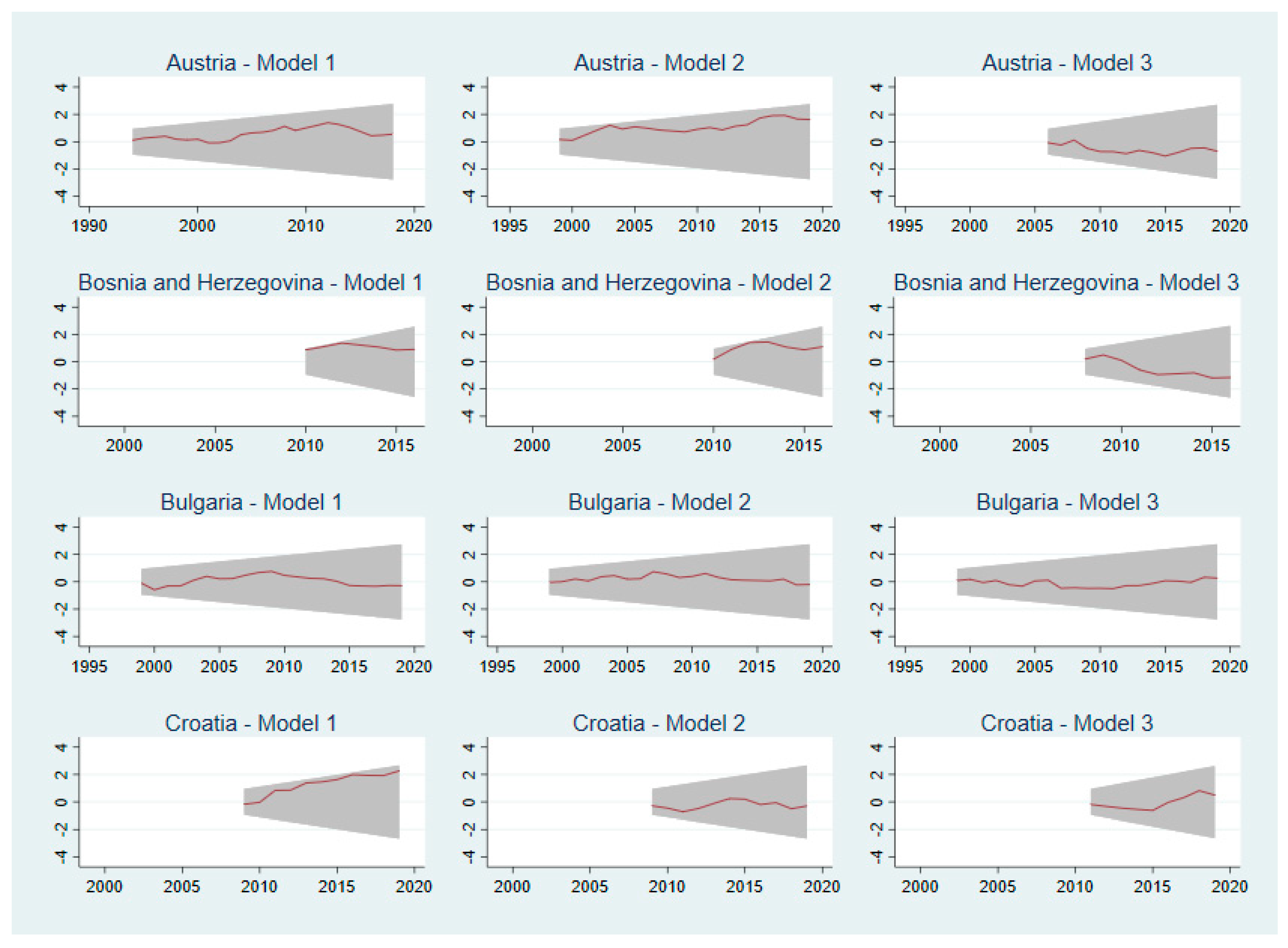
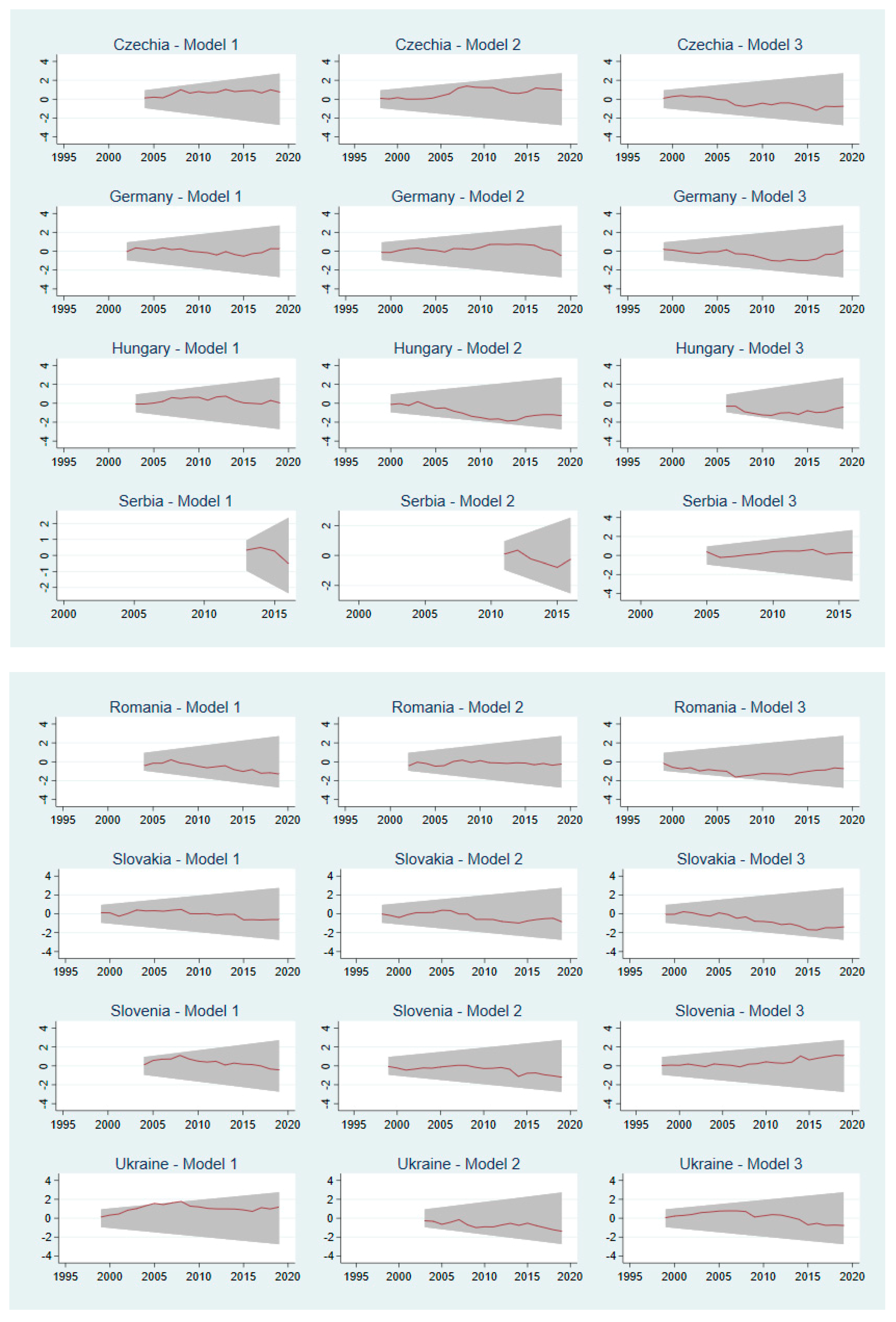
The validity of each model was verified by the diagnostic tests mentioned in Section 3.2. This implies that 26 of all 36 of the models are valid and safe to use for decision and policymaking. The stability of the models as depicted in Appendix A implies that they all fall within the 5% significance level boundary. The stability is proven in all models.

5. Discussion

As can be seen from Table 5, the analysis of the long-run and short-run relationship among economic growth, energy consumption and CO2 emissions in the Danube region countries reveal contrasting findings.
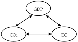
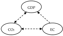
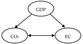
A bidirectional long-run causality between economic growth, energy consumption and CO2 emissions was found only in the case of Bosnia and Herzegovina, which supports the feedback hypothesis, indicating that these three macroeconomic variables are jointly determined and affect each other [62]. This finding corresponds with those of Liu et al. [63], who investigated the nexus between the three variables in emerging economies of China and India, and Odugbesan and Rjoub [51], who reported the same causality (including urbanisation) for Mexico.
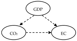
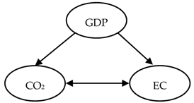
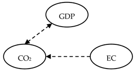
A unidirectional causality running from GDP to CO2 and energy consumption to CO2 is present in the case of Austria, Croatia, Czech Republic, Serbia, Slovakia, Slovenia and Ukraine, supporting the growth hypothesis. This implies that economic growth, as well as the increase in energy consumption, may result in an increase in CO2 emissions. This is consistent with the findings of [63] for Japan and [64] for Japan and the United Kingdom, which point out that economic growth in these countries is accompanied by an increase in CO2 emissions. The introduction of decarbonisation and energy efficiency measures will play an important role in these countries. A bidirectional causal relationship between these two variables is present only in Bosnia and Herzegovina.
Going back to the hypotheses formulated in the introduction, hypothesis 1 was confirmed in the case of Austria, Bosnia and Herzegovina, Croatia, the Czech Republic, Slovakia, Slovenia and Ukraine. In these countries, a long-run relationship from GDP to CO2 has been demonstrated.
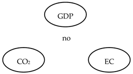
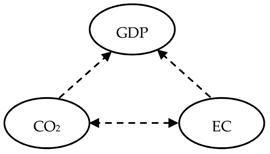
No causal relationship from long-run perspective was found between the three variables in the cases of Bulgaria, Germany, Hungary and Romania. This confirms hypothesis 3, stating that there will be countries within the Danube region for which there will be no long-term relationship between the variables GDP, energy consumption and CO2 emissions. These findings imply that energy consumption and economic growth do not have a significant effect on the production of carbon emissions. On the other hand, decarbonisation measures in these countries would have only a minimal impact on economic growth. These findings are consistent with Chukwunonso Bosah et al. [64], who reported similar results for Algeria, Cameroon, Ghana, Canada, the USA, France and India.
The long-run bidirectional causal relationship was found between energy consumption and CO2 emissions in Bosnia and Herzegovina, Croatia, Serbia and Slovenia. The long-run unidirectional relationship was found between energy consumption and CO2 emissions in Austria, Czech Republic, Slovakia and Ukraine. These findings support hypothesis 2, stating that in most countries of the examined region, a long-run relationship from energy consumption to CO2 emissions will be demonstrated.
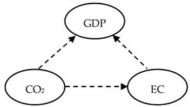
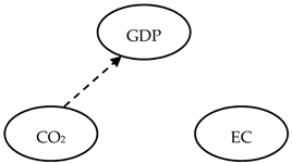
From the short-run perspective, very heterogeneous results can be found in terms of causality among the variables. The short-run unidirectional causality was found in Croatia, Czech Republic, Germany, Slovakia, Slovenia and Ukraine, running from CO2 to GDP. Bidirectional causality between the two variables is present in Romania and Serbia. A causal relationship is absent in the case of Hungary, Bulgaria and Bosnia and Herzegovina.
Short-run unidirectional causality running from energy consumption to GDP was found in case of Bosnia and Herzegovina, Croatia, Germany, Romania and Slovakia. This result confirms the growth hypothesis implying that an increase in energy consumption may contribute to economic growth. Similar results are reported by Narayan and Smyth [65] for G7 countries and by Odugbesan and Rjoub [51] for Nigeria and Indonesia.
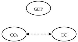
The feedback hypothesis was confirmed in Bosnia and Herzegovina, Bulgaria, Croatia, Germany, Hungary and Romania the in short-run, where bidirectional relationships can be found between energy consumption and CO2 emissions, indicating that energy consumption has intensified CO2 emissions in these countries. This finding is consistent with the results of [64], who confirmed the feedback effect in some African countries, Italy, Japan and the UK.

6. Conclusions

The issue of the reduction in energy use, as well as meeting the decarbonisation objectives, directly affects all European Union member states, whose vision is to reduce energy consumption and reduce CO2 emissions in order to become the first carbon-neutral continent. In this study, we focused on the Danube region countries, which create a very heterogeneous group in terms of geographic, economic, cultural and socio-demographic characteristics. Despite these differences, they have great potential to improve in many areas, including the energy sector, where they can increase their energy efficiency, improve energy infrastructure and foster the use of renewable energy sources. Results of the analysis reveal heterogeneous long-run and short-run causal relationship between three variables: economic growth, energy consumption, and CO2 emissions. Countries were split into different categories in terms of unidirectional and bidirectional relationships among variables. In cases where the unidirectional impact of GDP and energy consumption on CO2 emissions has been identified, we recommend focusing on promoting energy efficiency and increasing the share of renewable energy sources.
Like all studies, this one has its limitations. One of the most limiting factors was the shortness of the time series in some non-EU countries, which resulted from both the historical context and the unavailability and inconsistency of data. The authors have the ambition to repeat the analysis several years apart when the time series will be longer, which will also support the credibility of the models. The spectrum of variables can be expanded in the future, e.g., by the ratio of renewables in the energy mix or the energy dependence of countries.
The results of our research clearly point to the interconnectedness of energy, economic growth and CO2 emissions. In the light of these findings, it is, therefore, necessary to formulate and implement integrated policies that do not jeopardise the economic prosperity of the region but at the same time ensure good environmental condition and the sustainability of the energy system.
The results also contribute to the information base essential for making responsible and informed decisions by policymakers and other stakeholders in individual countries and together fulfil the objectives of the EU Strategy for the Danube Region. Moreover, they can serve as a platform for mutual cooperation and cohesion among countries in this region.

Supplementary Materials

The following are available online at https://www.mdpi.com/article/10.3390/en14113165/s1, Table S1: Dataset.

Author Contributions

Conceptualization, data curation, writing—original draft preparation, supervision, E.L. and J.C.; methodology, software, validation, formal analysis, E.L.; investigation, resources, J.C. All authors have read and agreed to the published version of the manuscript.

Funding

Scientific Grant Agency of the Ministry of Education, Science, Research and Sport of the Slovak Republic and the Slovak Academy of Sciences (1/0508/21).

Institutional Review Board Statement

Not applicable.

Informed Consent Statement

Not applicable.

Data Availability Statement

Data used in this study were extracted from publicly available databases: World Bank: GDP per capita in constant 2010 USD (https://databank.worldbank.org/reports.aspx?source=2&series=NY.GDP.PCAP.KD&country=, accessed on 24 May 2021); the Global Carbon Project: CO2 per capita in tons (http://www.globalcarbonatlas.org/en/CO2-emissions, accessed on 24 May 2021) and BP Statistical Review of World Energy: energy consumption per capita in kWh (https://www.bp.com/en/global/corporate/energy-economics/statistical-review-of-world-energy.html, accessed on 24 May 2021).

Acknowledgments

The authors also thank the journal editor and anonymous reviewers for their guidance and constructive suggestions.

Conflicts of Interest

The authors declare no conflict of interest.

Appendix A

Recursive cusum plot of dependent variable, with 95% confidence bands around the null.
Figure A1. The cumulative sum of recursive residuals (CUSUM) plots.
Energies 14 03165 g0a1aEnergies 14 03165 g0a1b

References

  1. OECD. Economic Policies to Foster Green Growth; OECD: Paris, France, 2014. [Google Scholar]
  2. UNEP. Green Economy—What Is GEI? UNEP: Nairobi, Kenya, 2014. [Google Scholar]
  3. United Nations. Transforming Our World: The 2030 Agenda for Sustainable Development; United Nations: New York, NY, USA, 2015.
  4. European Commission. The European Green Deal. European Commission; European Commission: Brussels, Belgium, 2019. [Google Scholar] [CrossRef]
  5. European Commission. Powering a Climate-Neutral Economy: An EU Strategy for Energy System Integration. Communication from the Commission to the European Parliament, the Council, the European Economic and Social Committee and the Committee of the Regions. Available online: https://ec.europa.eu/energy/sites/ener/files/energy_system_integration_strategy_pdf (accessed on 1 March 2021).
  6. European Commission. A Hydrogen Strategy for a Climate-Neutral Europe. Communication from the Commission to the European Parliament, the Council, the European Economic and Social Committee and the Committee of the Regions. Available online: https://ec.europa.eu/energy/sites/ener/files/hydrogen_strategy.pdf (accessed on 1 March 2021).
  7. Hamilton, F.I.; Andrews, K.D.; Pichler-Milanovic, N. Transformation of Cities in Central and Eastern Europe: Towards Globalization; United Nations Publications: New York, NY, USA, 2005. [Google Scholar]
  8. Giffinger, R.; Suitner, J. Danube region strategy—Arguments for a territorial capital based multilevel approach. Spat. Int. Rev. 2005, 23, 9–16. [Google Scholar] [CrossRef]
  9. Borowski, P.F. Zonal and Nodal Models of energy market in European Union. Energies 2020, 13, 4182. [Google Scholar] [CrossRef]
  10. Ferrer, J.N.; Mihnea, C.; Stroia, C.; Bryhn, J. Comparative Study on the Governance Structure and Energy Policies in EU Macro-Regional Strategies. Available online: https://www.ceps.eu/wp-content/uploads/2019/07/RR2019-02_EU-macroregional-strategies.pdf (accessed on 5 March 2021).
  11. Chalvatzis, K.J.; Ioannidis, A. Energy supply security in the EU: Benchmarking diversity and dependence of primary energy. Appl. Energy 2017, 207, 465–476. [Google Scholar] [CrossRef]
  12. Hawker, G.; Bell, K.; Gill, S. Electricity security in the European Union—The conflict between national capacity mechanisms and the single market. Energy Res. Soc. Sci. 2017, 24, 51–58. [Google Scholar] [CrossRef] [Green Version]
  13. Siksnelyte, I.; Zavadskas, E.K.; Bausys, R.; Streimikiene, D. Implementation of EU energy policy priorities in the Baltic Sea Region countries: Sustainability assessment based on neutrosophic MULTIMOORA method. Energy Policy 2019, 125, 90–102. [Google Scholar] [CrossRef] [Green Version]
  14. De Bruyn, S.M.; Van Den Bergh, J.C.J.M.; Opschoor, J.B. Economic growth and emissions: Reconsidering the empirical basis of environmental Kuznets curves. Ecol. Econ. 1998. [Google Scholar] [CrossRef]
  15. Heiskanen, E.; Jalas, M. Dematerialization through Services—A Review and Evaluation of the Debate; The Finnish Environment: Helsinki, Finland, 2000. [Google Scholar]
  16. Vehmas, J.; Luukkanen, J.; Kaivo-Oja, J. Linking analyses and environmental Kuznets curves for aggregated material flows in the EU. J. Clean. Prod. 2007, 15, 1662–1673. [Google Scholar] [CrossRef]
  17. Szulecki, K. European energy governance and decarbonization policy: Learning from the 2020 strategy. Clim. Policy 2016, 16, 543–547. [Google Scholar] [CrossRef]
  18. Steger, S.; Bleischwitz, R. Decoupling GDP from resource use, resource productivity and competitiveness: A cross-country comparison. In Sustainable Growth and Resource Productivity: Economic and Global Policy Issues; Routledge: London, UK, 2017. [Google Scholar] [CrossRef]
  19. Chovancová, J.; Tej, J. Decoupling economic growth from greenhouse gas emissions: The case of the energy sector in V4 countries. Equilibrium 2020, 15, 235–251. [Google Scholar] [CrossRef]
  20. Sanyé-Mengual, E.; Secchi, M.; Corrado, S.; Beylot, A.; Sala, S. Assessing the decoupling of economic growth from environmental impacts in the European Union: A consumption-based approach. J. Clean. Prod. 2019, 236, 117535. [Google Scholar] [CrossRef]
  21. Zhang, Y.; Song, W.; Fu, S.; Yang, D. Decoupling of land use intensity and ecological environment in Gansu province, China. Sustainability 2020, 12, 2779. [Google Scholar] [CrossRef] [Green Version]
  22. Finel, N.; Tapio, P. Decoupling Transport CO2 from GDP; Finland Futures Research Centre Ebook: Turku, Finland, 2012. [Google Scholar]
  23. Tapio, P. Towards a theory of decoupling: Degrees of decoupling in the EU and the case of road traffic in Finland between 1970 and 2001. Transp. Policy 2005, 12, 137–151. [Google Scholar] [CrossRef] [Green Version]
  24. Ru, X.; Chen, S.; Dong, H. An empirical study on relationship between economic growth and carbon emissions based on decoupling theory. J. Sustain. Dev. 2012, 5, 43. [Google Scholar] [CrossRef]
  25. Jiang, X.T.; Su, M.; Li, R. Investigating the factors influencing the decoupling of transport-related carbon emissions from turnover volume in China. Sustainability 2018, 10, 3034. [Google Scholar] [CrossRef] [Green Version]
  26. Zhang, L.; Kou, C.; Zheng, J.; Li, Y. Decoupling analysis of CO2 emissions in transportation sector from economic growth during 1995–2015 for six cities in Hebei, China. Sustainability 2018, 10, 4149. [Google Scholar] [CrossRef] [Green Version]
  27. Wang, Q.; Wang, S.; Li, R. Determinants of decoupling economic output from carbon emission in the transport sector: A comparison study of four municipalities in China. Int. J. Environ. Res. Public Health 2019, 16, 3729. [Google Scholar] [CrossRef] [Green Version]
  28. Zhang, X.; Ke, S. Linkage Analysis of the Resources, Population, and Economy in China’s Key State-Owned Forest Areas. Sustainability 2020, 12, 3855. [Google Scholar] [CrossRef]
  29. Balcilar, M.; Ozdemir, Z.A.; Tunçsiper, B.; Ozdemir, H.; Shahbaz, M. On the nexus among carbon dioxide emissions, energy consumption and economic growth in G-7 countries: New insights from the historical decomposition approach. Environ. Dev. Sustain. 2020, 22, 8097–8134. [Google Scholar] [CrossRef]
  30. Apergis, N.; Payne, J.E. Renewable energy consumption and economic growth: Evidence from a panel of OECD countries. Energy Policy 2010, 32, 1392–1397. [Google Scholar] [CrossRef]
  31. Apergis, N.; Payne, J.E. Energy consumption and economic growth in Central America: Evidence from a panel cointegration and error correction model. Energy Econ. 2009, 69, 2255–2260. [Google Scholar] [CrossRef]
  32. Ozturk, I.; Aslan, A.; Kalyoncu, H. Energy consumption and economic growth relationship: Evidence from panel data for low and middle income countries. Energy Policy 2010, 38, 4422–4428. [Google Scholar] [CrossRef]
  33. Fan, W.; Meng, M.; Lu, J.; Dong, X.; Wei, H.; Wang, X.; Zhang, Q. Decoupling Elasticity and Driving Factors of Energy Consumption and Economic Development in the Qinghai-Tibet Plateau. Sustainability 2020, 12, 1326. [Google Scholar] [CrossRef] [Green Version]
  34. Omri, A. An international literature survey on energy-economic growth nexus: Evidence from country-specific studies. Renew. Sustain. Energy Rev. 2014, 38, 951–959. [Google Scholar] [CrossRef] [Green Version]
  35. Kan, S.; Chen, B.; Chen, G. Worldwide energy use across global supply chains: Decoupled from economic growth? Appl. Energy 2019, 250, 1235–1245. [Google Scholar] [CrossRef]
  36. Vural, G. Renewable and non-renewable energy-growth nexus: A panel data application for the selected Sub-Saharan African countries. Resour. Policy 2020, 65, 101568. [Google Scholar] [CrossRef]
  37. Ozturk, I.; Al-Mulali, U. Natural gas consumption and economic growth nexus: Panel data analysis for GCC countries. Renew. Sustain. Energy Rev. 2015, 51, 998–1003. [Google Scholar] [CrossRef]
  38. Ozcan, B.; Ari, A. Nuclear energy-economic growth nexus in OECD countries: A panel data analysis. J. Econ. Manag. Perspect. 2017, 11, 138–154. [Google Scholar]
  39. Shahbaz, M.; Shafiullah, M.; Papavassiliou, V.G.; Hammoudeh, S. The CO2–growth nexus revisited: A nonparametric analysis for the G7 economies over nearly two centuries. Energy Econ. 2017, 65, 183–193. [Google Scholar] [CrossRef] [Green Version]
  40. Zhou, X.; Zhang, M.; Zhou, M.; Zhou, M. A comparative study on decoupling relationship and influence factors between China’s regional economic development and industrial energy-related carbon emissions. J. Clean. Prod. 2017, 142, 783–800. [Google Scholar] [CrossRef]
  41. Naminse, E.; Zhuang, J. Economic Growth, Energy Intensity, and Carbon Dioxide Emissions in China. Pol. J. Environ. Stud. 2018, 27, 2193–2201. [Google Scholar] [CrossRef]
  42. Chovancová, J.; Vavrek, R. (De)coupling Analysis with Focus on Energy Consumption in EU Countries and Its Spatial Evaluation. Pol. J. Environ. Stud. 2020, 29, 2091–2100. [Google Scholar] [CrossRef]
  43. Yang, Y.; Jia, J.; Chen, C. Residential Energy-Related CO2 Emissions in China’s Less Developed Regions: A Case Study of Jiangxi. Sustainability 2020, 12, 2000. [Google Scholar] [CrossRef] [Green Version]
  44. Sadorsky, P. Energy related CO2 emissions before and after the financial crisis. Sustainability 2020, 12, 3867. [Google Scholar] [CrossRef]
  45. Turner, K.; Hanley, N. Energy efficiency, rebound effects and the environmental Kuznets Curve. Energy Econ. 2011, 33, 709–720. [Google Scholar] [CrossRef] [Green Version]
  46. Dogan, E.; Turkekul, B. CO2 emissions, real output, energy consumption, trade, urbanization and financial development: Testing the EKC hypothesis for the USA. Environ. Sci. Pollut. Res. 2016, 23, 1203–1213. [Google Scholar] [CrossRef] [PubMed]
  47. Balado-Naves, R.; Baños-Pino, J.F.; Mayor, M. Do countries influence neighbouring pollution? A spatial analysis of the EKC for CO2 emissions. Energy Policy 2018, 123, 266–279. [Google Scholar] [CrossRef]
  48. Ang, J.B. CO2 emissions, energy consumption, and output in France. Energy Policy 2007, 30, 271–278. [Google Scholar] [CrossRef]
  49. Tiba, S.; Omri, A. Literature survey on the relationships between energy, environment and economic growth. Renew. Sustain. Energy Rev. 2017, 69, 1129–1146. [Google Scholar] [CrossRef]
  50. Zhang, X.; Zhang, H.; Yuan, J. Economic growth, energy consumption, and carbon emission nexus: Fresh evidence from developing countries. Environ. Sci. Pollut. Res. 2019, 26, 26367–26380. [Google Scholar] [CrossRef]
  51. Odugbesan, J.A.; Rjoub, H. Relationship among economic growth, energy consumption, CO2 emission, and urbanization: Evidence from MINT countries. Sage Open 2020, 10, 2158244020914648. [Google Scholar] [CrossRef] [Green Version]
  52. Raggad, B. Carbon dioxide emissions, economic growth, energy use, and urbanization in Saudi Arabia: Evidence from the ARDL approach and impulse saturation break tests. Environ. Sci. Pollut. Res. 2018, 25, 14882–14898. [Google Scholar] [CrossRef]
  53. Farhani, S.; Ozturk, I. Causal relationship between CO2 emissions, real GDP, energy consumption, financial development, trade openness, and urbanization in Tunisia. Environ. Sci. Pollut. Res. 2015, 22, 15663–15676. [Google Scholar] [CrossRef]
  54. Dickey, D.A.; Fuller, W.A. Distribution of the estimators for autoregressive time series with a unit root. J. Am. Stat. Assoc. 1979, 74, 427–431. [Google Scholar]
  55. Kwiatkowski, D.; Phillips, P.C.B.; Schmidt, P.; Shin, Y. Testing the null hypothesis of stationarity against the alternative of a unit root: How sure are we that economic time series have a unit root? J. Econom. 1992, 54, 159–178. [Google Scholar] [CrossRef]
  56. Pesaran, M.H.; Shin, Y.; Smith, R.J. Bounds testing approaches to the analysis of level relationships. J. Appl. Econom. 2001, 16, 289–326. [Google Scholar] [CrossRef]
  57. Kripfganz, S.; Schneider, D.C. Response surface regressions for critical value bounds and approximate p-values in equilibrium correction models. Oxf. Bull. Econ. Stat. 2020, 82, 1456–1481. [Google Scholar] [CrossRef]
  58. Pesaran, M.H.; Shin, Y. An autoregressive distributed lag modelling approach to cointegration analysis. In Proceedings of the Symposium at the Centennial of Ragnar Frisch, the Norwegian Academy of Science and Letters, Oslo, Norway, 3–5 March 1995; pp. 371–413. [Google Scholar]
  59. Baum, C.F. Stata: The language of choice for time-series analysis? Stata J. 2005, 5, 46–63. [Google Scholar] [CrossRef] [Green Version]
  60. Hobijn, B.; Franses, P.H.; Ooms, M. Generalizations of the KPSS-Test for Stationarity; Econometric Institute Report 9802/A; Econometric Institute, Erasmus University Rotterdam: Rotterdam, The Netherlands, 1998. [Google Scholar]
  61. Türsoy, T. Causality between stock prices and exchange rates in Turkey: Empirical evidence from the ARDL bounds test and a combined cointegration approach. Int. J. Financ. Stud. 2017, 5, 8. [Google Scholar] [CrossRef] [Green Version]
  62. Magazzino, C. The relationship between real GDP, CO2 emissions, and energy use in the GCC countries: A time series approach. Cogent Econ. Financ. 2016, 4, 1152729. [Google Scholar] [CrossRef]
  63. Liu, H.; Lei, M.; Zhang, N.; Du, G. The causal nexus between energy consumption, carbon emissions and economic growth: New evidence from China, India and G7 countries using convergent cross mapping. PLoS ONE 2019, 14, e0217319. [Google Scholar] [CrossRef]
  64. Chukwunonso Bosah, P.; Li, S.; Kwaku Minua Ampofo, G.; Akwasi Asante, D.; Wang, Z. The nexus between electricity consumption, economic growth, and CO2 emission: An asymmetric analysis using nonlinear ARDL and nonparametric causality approach. Energies 2020, 13, 1258. [Google Scholar] [CrossRef] [Green Version]
  65. Narayan, P.K.; Smyth, R. Energy consumption and real GDP in G7 countries: New evidence from panel cointegration with structural breaks. Energy Econ. 2008, 30, 2331–2341. [Google Scholar] [CrossRef]
Figure 1. Plot of CO2 emissions, energy consumption and GDP for Danube region countries.
Energies 14 03165 g001aEnergies 14 03165 g001b
Table 1. Descriptive statistics.
GDP per CapitaPer Capita CO2 Emissions Energy Consumption per Capita
nMeanMinimumMaximumStd. Dev.nMeanMinimumMaximumStd. Dev.nMeanMinimumMaximumStd. Dev.
AT3036,789.2417,634.5368,150.1117,892.76308.2867.4399.5940.6173046,652.3342,664.2050,621.482254.917
BH263359.70319.016108.511934.13304.3680.8148.0651.8142517,226.607641.6524,397.524741.948
BG304524.791148.499828.152982.73306.5825.6658.6750.5873029,741.4926,584.9936,510.572025.429
HR2510,560.154841.5916,296.814056.02304.5063.4815.6960.6223021,877.2416,847.9524,910.582330.444
CZ3012,927.162896.6123,494.607345.483011.8399.45015.8791.5283047,113.0843,317.3852,778.712459.065
DE3035,068.2122,303.9647,959.999001.183010.7698.40513.3121.0683047,967.8743,703.3852,872.982129.842
HU299682.843350.2616,731.824688.72305.6444.4447.0800.6373027,931.7324,560.7831,349.121502.863
MO205711.761627.078908.932336.99301.8600.8506.3631.384259517.877428.6317,673.632247.433
ME251864.02399.624503.521322.17303.0121.9714.1950.6091121,309.1418,880.7926,932.862409.799
SR254659.06914.797411.842014.25305.1303.7366.6540.8162520,644.2313,785.3223,829.862432.372
RO305479.761102.1012,919.534076.15304.7363.8187.2070.7873021,118.1418,010.1631,213.362757.741
SK3011,100.082405.5419,406.356361.32307.7266.10511.6551.1803038,001.2332,904.9946,765.893164.200
SI3016,883.706562.0227,483.347143.82307.6896.5479.0060.6743038,933.5231,935.4545,695.763126.459
UA302019.46635.704029.711122.81307.0934.98413.7152.1073033,351.7521,501.2261,620.089212.049
Table 2. Augmented Dickey–Fuller unit-root test.
Country LGDPCO2LEC
LevelFirst DifferenceLevelFirst DifferenceLevelFirst Difference
AustriaAT−0.694−3.923 **−1.388−5.993 ***−2.204−8.166 ***
Bosnia and HerzegovinaBH−5.939 ***−3.081 *0.007−4.751 ***−1.634−7.637 ***
BulgariaBG−0.276−7.166 ***−5.082 ***−6.114 ***−4.770 ***−6.148 ***
CroatiaHR−1.232−2.970 *−1.393−6.704 ***−1.371−5.746 ***
CzechiaCZ−0.878−5.103 ***−2.558−5.636 ***−2.533−5.232 ***
GermanyDE−1.213−4.551 ***−1.109−6.339 ***−1.748−8.602 ***
HungaryHU−1.163−3.689 **−2.248−4.935 ***−2.636−4.386 ***
MoldovaMO−2.849−2.919 *−7.396 ***−4.262 ***−4.264 ***−3.979 **
MontenegroME0.066−3.688 **−2.253−9.797 ***−4.528 ***−6.131 ***
SerbiaSR−1.382−5.482 ***−2.483−6.992 ***−2.642−5.893 ***
RomaniaRO0.064−3.929 **−3.672 **−5.074 ***−4.337 ***−4.565 ***
SlovakiaSK−2.106−3.317 *−4.923 ***−5.491 ***−2.407−7.161 ***
SloveniaSI−0.670−4.936 ***−0.871−4.888 ***−1.885−6.057 ***
UkraineUA−0.438−3.364 *−5.454 ***−3.286 *−1.421−3.762 **
Note: The significance of the ADF test is indicated by an asterisk in the table where *, **, *** denotes 5%, 1%, and 0.1% significance level, respectively.
Table 3. The ARDL bound testing for cointegration with Kripfganz and Schneider [57] critical values and approximate p-values.
Country VariableF-StatisticI (0) Bound (5%)I (1) Bound (5%)CointegrationDecision
AustriaATLGDP4.1644.3645.613Noshort-run model
CO214.3064.3665.666Yeserror correction model
LEC4.8204.3785.935Noshort-run model
Bosnia and HerzegovinaBHLGDPcrashed error correction model
CO2crashed error correction model
LECcrashed error correction model
BulgariaBGLGDP0.5574.3645.613Noshort-run model
CO21.5094.3665.666Noshort-run model
LEC1.7904.3665.666Noshort-run model
CroatiaHRLGDP11.1694.7056.435Yeserror correction model
CO214.4444.7056.435Yeserror correction model
LECcrashed error correction model
CzechiaCZLGDP5.5584.3645.613Noshort-run model
CO221.7474.3645.613Yeserror correction model
LEC4.0154.3665.666Noshort-run model
GermanyDELGDP0.4424.3645.613Noshort-run model
CO20.7014.3665.666Noshort-run model
LEC2.3724.3665.666Noshort-run model
HungaryHULGDP1.5684.3975.660Noshort-run model
CO23.0464.4075.778Noshort-run model
LEC2.0914.4025.719Noshort-run model
SerbiaSRLGDPcrashed short-run model
CO2crashed error correction model
LEC21.5334.8556.415Yeserror correction model
RomaniaROLGDP1.7834.3665.666Noshort-run model
CO21.1624.3735.828Noshort-run model
LEC2.3654.3665.666Noshort-run model
SlovakiaSKLGDP3.1364.3695.720Noshort-run model
CO27.6484.3645.613Yeserror correction model
LEC2.9144.3665.666Noshort-run model
SloveniaSILGDP0.5244.3665.666Noshort-run model
CO27.5384.3665.666Yeserror correction model
LEC23.9354.3645.613Yeserror correction model
Ukraine UA LGDP4.9664.3695.720Noshort-run model
CO218.004.3768.882Yeserror correction model
LEC4.4284.3665.666Noshort-run model
Table 4. Long-run statistics and Diagnostic test.
Long-Run Statistics Diagnostic Test
DependentLGDPtCO2tLECtECTNormalitySer. CorrHomoskedasticityStability
Variable p-Valuep-Valuep-Value
ATΔLGDPt 0.870.510.48stable
ΔCO2t−0.56 ** 10.50 ***−0.61 ***0.100.760.82stable
ΔLECt 0.610.01 **0.41stable
BHΔLGDPt 0.43 ***−2.59 *−0.38 *0.270.440.39stable
ΔCO2t1.99 *** 3.39 *−1.10 **0.01 **0.02 *0.39stable
ΔLECt−0.40 ***0.25 *** −2.00 **0.640.750.39stable
BGΔLGDPt 0.610.490.02 *stable
ΔCO2t 0.340.250.88stable
ΔLECt 0.460.630.78stable
HRΔLGDPt −3.5045.21−0.090.00 ***0.670.40stable
ΔCO2t−0.80 ** 12.38 ***−0.92 **0.00 ***0.190.40stable
ΔLECt0.05 **0.08 *** −2.17 ***0.00 ***0.330.40stable
CZΔLGDPt 0.760.090.41stable
ΔCO2t−1.64 *** 15.54 ***−0.64 ***0.180.530.12stable
ΔLECt 0.650.920.71stable
DEΔLGDPt 0.930.780.41stable
ΔCO2t 0.070.410.47stable
ΔLECt 0.820.600.73stable
HUΔLGDPt 0.870.990.40stable
ΔCO2t 0.190.630.26stable
ΔLECt 0.440.080.40stable
SRΔLGDPt 0.00 **0.520.39stable
ΔCO2t−0.52 * 12.31 **−1.68 *0.00 ***0.03 *0.39stable
ΔLECt0.020.04 ** −1.37 ***0.00 ***0.220.39stable
ROΔLGDPt 0.480.770.41stable
ΔCO2t 0.610.110.41stable
ΔLECt 0.150.730.05stable
SKΔLGDPt 0.660.920.82stable
ΔCO2t−0.38 * 7.85 ***−0.49 ***0.050.990.29stable
ΔLECt 0.620.440.64stable
SIΔLGDPt 0.360.310.41stable
ΔCO2t−1.04 ** 11.41 ***−0.59 **0.400.820.96stable
ΔLECt0.07 ***0.08 *** −0.84 ***0.990.100.19stable
UA ΔLGDPt 0.200.410.76stable
ΔCO2t0.39 ** 4.22 ***−0.57 ***0.00 ***0.650.41stable
ΔLECt 0.850.650.22stable
Note: The significance of the coefficients is indicated by an asterisk in the tables where *, **, *** denotes 5%, 1%, and 0.1% significance level, respectively.
Table 5. Relationship between variables.
CountryLong-RunShort-Run
AT Energies 14 03165 i001 Energies 14 03165 i002
BH Energies 14 03165 i003 Energies 14 03165 i004
BG Energies 14 03165 i005 Energies 14 03165 i006
HR Energies 14 03165 i007 Energies 14 03165 i008
CZ Energies 14 03165 i009 Energies 14 03165 i010
DE Energies 14 03165 i011 Energies 14 03165 i012
HU Energies 14 03165 i013 Energies 14 03165 i014
SR Energies 14 03165 i015 Energies 14 03165 i016
RO Energies 14 03165 i017 Energies 14 03165 i018
SK Energies 14 03165 i019 Energies 14 03165 i020
SI Energies 14 03165 i021 Energies 14 03165 i022
UA Energies 14 03165 i023 Energies 14 03165 i024
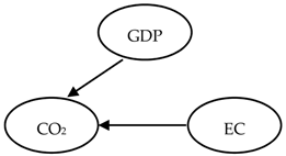
Note 1: Energies 14 03165 i025 Uni-directional long-run relationship; Energies 14 03165 i026 Bi-directional long-run relationship; Energies 14 03165 i027 Uni-directional short-run relationship; Energies 14 03165 i028 Bi-directional short-run relationship. Note 2: GDP—gross domestic product, CO2—carbon dioxide, EC—energy consumption.
Table 6. Short-run statistics.
Short-Run Statistics
DependentΔLGDP ΔCO2 ΔLEC
Variablett−1t−2t−3t−4tt−1t−2t−3t−4tt−1t−2t−3t−4
ATΔLGDPt 0.37 0.14 −0.44
ΔCO2t1.28 ***
ΔLECt0.02−0.040.060.15 ****0.03 **−0.02 −0.13−0.060.230.43 **
BHΔLGDPt −0.12−0.78 ** −0.02−0.09 0.80 **0.22−0.24−0.29 *
ΔCO2t1.55−0.742.45 0.51 * −2.49−1.261.101.57 **
ΔLECt −0.30 *−0.33 **−0.20 *−0.05 0.93 **0.45 *
BGΔLGDPt −0.28 0.01 0.07
ΔCO2t0.01 0.003 6.95 ***
ΔLECt0.02 0.10 *** −0.07
HRΔLGDPt 0.46 **0.47 *** −2.46 *−2.66 **−1.83 **−1.14 **
ΔCO2t 0.42 *−0.04−1.07 ** −5.89 **−3.46 *−2.55 *
ΔLECt0.14 −0.10−0.13 *−0.000.13 ** 0.94 *0.64 *0.26
CZΔLGDPt 0.30−0.330.63 **−0.27 *0.060.060.15 * 1.38
ΔCO2t
ΔLECt0.10 * 0.06 ** −0.14
DEΔLGDPt 0.54 *−0.50 *0.35−0.390.37 * −3.64 *
ΔCO2t0.46 0.04 10.97 ***
ΔLECt−0.03 0.08 *** −0.13
HUΔLGDPt 0.62 **−0.430.70 *−0.400.36 −1.47
ΔCO2t0.17 −0.04 4.80 ***
ΔLECt−0.03−0.002−0.020.13 * 0.14 ***0.040.08 * −0.15−0.43 *
SRΔLGDPt −0.880.170.500.210.220.52 *0.42 * −2.52−1.70−0.15−3.06−2.30
ΔCO2t2.15 *2.86 *0.80 −0.21−0.45 −11.72−11.40 *−10.01
ΔLECt 0.51 **0.39 *
ROΔLGDPt 0.18 0.36 *0.35 * −0.28−2.13 **0.76 *1.54 **−0.49
ΔCO2t0.73 * −0.48 *−0.25 *−0.23 * 0.89 ***3.02 **
ΔLECt0.03 0.14 *** −0.11
SKΔLGDPt 0.45 * 0.23 * −0.49 *
ΔCO2t
ΔLECt−0.06 0.10 ** −0.28
SIΔLGDPt 0.09−0.40 * 0.070.090.080.11 *−0.11 *0.62
ΔCO2t0.77
ΔLECt
UAΔLGDPt 0.27 * 0.34 ** 0.44
ΔCO2t0.59 *0.58 * −0.31 **−0.12 * 1.26
ΔLECt0.03 0.11 ** −0.09
Note: The significance of the coefficients is indicated by an asterisk in the tables, where *, **, *** denotes 5%, 1%, and 0.1% significance level, respectively.
Publisher’s Note: MDPI stays neutral with regard to jurisdictional claims in published maps and institutional affiliations.