
Multi-Step Energy Demand and Generation Forecasting with Confidence Used for Specification-Free Aggregate Demand Optimization


Abstract
1. Introduction
- The end user is an energy consumer who views the recommendations about the time points in the near future when energy consumption should be preferred according to the desired weighting factors of the three optimization criteria and the unit prices of energy at every time point which are applicable to this user, and adjusts his/her consumption behavior accordingly.
- The end user is a Distribution Systems Operator that forwards the recommendations of these algorithms to its customers.
- The end user is someone authorized to determine the unit prices of energy consumption at every time point, so (s)he can examine to what extent the economic criterion contradicts the renewable energy penetration and power stability criteria and adjust unit prices accordingly, also dynamically.
2. Related Work and Our Contribution
3. High-Level Architecture
4. The Forecasting Algorithm
4.1. Methodology of the Forecasting Algorithm
- Scaling each raw variable so that it has mean equal to 0 and standard deviation equal to 1. This is required by some of the non-linear regression architectures.
- In particular cases, the target variable is transformed to one of its features, but typically all raw variables are directly used in the following steps, just after aggregation.
- Selection of input variables based on linear regression.
- Grouping the historical dataset w.r.t. month and day of week by applying a clustering algorithm to the data of the target variable (i.e., the variable to be forecast). The selection of the clustering algorithm and respective clusters is automatic, based on the behavior of the target variable, and particularly the selection of algorithm is also based on training of linear regression approximations of the forecasting models.
- Supervised training of all regression architectures on the selected input variables. A separate training is performed for each group and forecasting horizon. The best architecture, based on 3-fold cross-validation, is automatically selected in each case, and the respective model is retrained within the whole historical dataset. (Cross-validation is a common method to evaluate the ability of a model to generalize to unknown data. Since usually about 50–70% of a dataset is used for a single training, considering 3 folds is a reasonable choice).
- t: time point for which the forecast is made
- s: forecasting horizon
- : estimation of the value that the target variable will have at the time point t based on the forecasting horizon s
- : the group of months and days of week that t belongs to
- : latest known measurement of the target variable within when forecasting for the time point t with horizon s (“present value”)
- r: duration such that all past values of the variable to be forecast, within , obtained after final aggregation (see Section 4.3.1), with a delay up to this duration, are used as input to the model
- : latest known measurement of the target variable at the same time of the day as t within when forecasting for the time point t with horizon s (“last value at same time”)
- : past values of the variable to be forecast, within , obtained after final aggregation, with a delay up to duration r, to be used as input to the model, when forecasting for the time point t with horizon s
- : historical mean of the target variable at the same time of the day as t within (“average time profile”)
- : weather variables at the time point t (forecast weather in case of real-time forecast of the target variable, or exact weather in case of training on a historical interval)
- : mean of weather variables within the interval from the time point of to t—in practice, no variable from this vector proved to be useful (and it would not make sense in most of the cases), so it will not be discussed later
4.1.1. Forecasting Regression Model Architectures and Tested Hyper-Parameters
- Multilayer Perceptron Regressor [MLP(hidden layer sizes)]—in case of absence of hidden layers [MLP()], this is reduced to linear regression
- -
- hidden layer sizes = (), (1), (2), (5), (1,1), (2,2), (5,5)
- -
- activation = “tanh”
- -
- solver = “lbfgs”
- -
- maximum number of iterations =
- -
- alpha = 0
- Random Forest Regressor [RF(maximum depth)]
- -
- maximum depth = 1, 2, 5, 10
- -
- number of estimators = 100
- Nearest Neighbour Regressor [NN(number of neighbours, weights)]
- -
- number of neighbours = 5, 10, 20, 50, 100, 200
- -
- weights = “uniform”, “distance”
- Support Vector Regressor [SVR(penalty, kernel(degree), epsilon)]
- -
- penalty (C) = 0.1, 1, 10
- -
- kernel = “poly” (polynomial), “rbf” [Radial Basis Function (RBF)], “sigmoid”
- -
- degree = 1, 2 (applicable only to the “poly” kernel)
- -
- epsilon = 0.1, 0.01, , ,
- -
- maximum number of iterations =
- Gaussian Process Regressor [GPR(alpha)] (when the number of data points is less than , so that training is memory-efficient)
- -
- alpha = , , , , , , , , 0.01, 0.1
- Kernel Regression [KR(kernel, gamma)]
- -
- kernel = “poly”, “rbf”, “sigmoid”
- -
- gamma = 0.01, 0.1, 1, 10, 100,
- Exteme Learning Machines [ELM(hidden layer units, alpha, RBF width, activation function)]
- -
- hidden layer units = 1, 2, 5, 10, 20, 50, 100
- -
- alpha = 0, 0.5, 1
- -
- RBF width = , 1
- -
- activation function = “gaussian”, “tanh”
4.1.2. Clustering Methodology and Relevant Architectures Tested
- Algorithms automatically selecting number of clusters:
- -
- Affinity Propagation (AP)
- -
- Mean Shift (MS)
- Algorithms requiring manual selection of number of clusters n (1, 2, 6 and 12 clusters are tested for month, whereas 1, 2 and 7 clusters are tested for day of week):
- -
- K-Means (KM(n))
- -
- Agglomerative Clustering (AC(n))
4.1.3. Evaluation
- F: training-test set split of the cross-validation
- : time interval for which forecasts are made based on horizon s, within all training/test sets obtained by split F when computing training/test NRMSE respectively and within all groups of months and days of week pairs resulting from clustering
- : exact value of the target variable at the time point t
- : forecast value of the target variable for the time point t
- : mean of the target variable within the whole historical dataset
4.2. Raw Data Used from Each Demonstrator
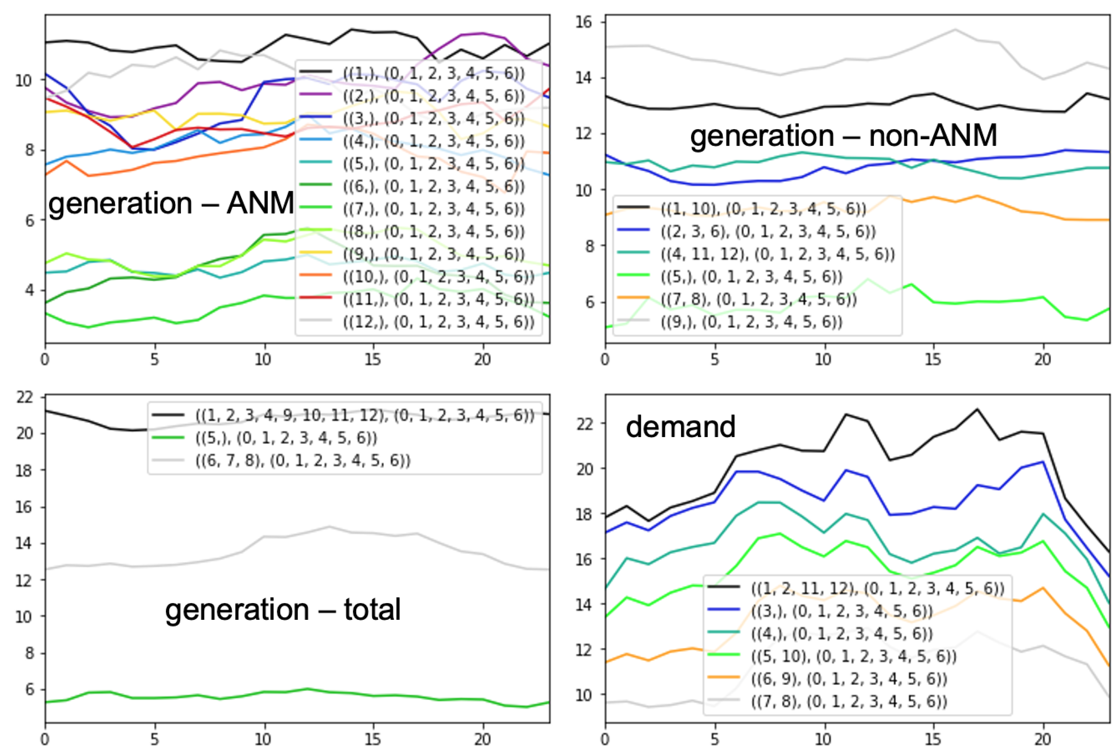
- Orkney generation was frozen within some intervals, which were discarded from the analysis. After that, about 5% and 6% of ANM and non-ANM generation timestamps respectively appeared to have missing values. Furthermore, a few negative values of generation were replaced by 0.
- In Madeira case, about 1% of the timestamps were discarded, because the sum of registered total demand was not within the range of the total generation, renewable and non-renewable (thermal), although total demand and total generation should be equal.
4.3. Experimental Results from the Forecasting Algorithm and Discussion
4.3.1. Algorithmic Specifications and Initial Pre-Processing
4.3.2. Input Variables Selection and Timestamps Clustering
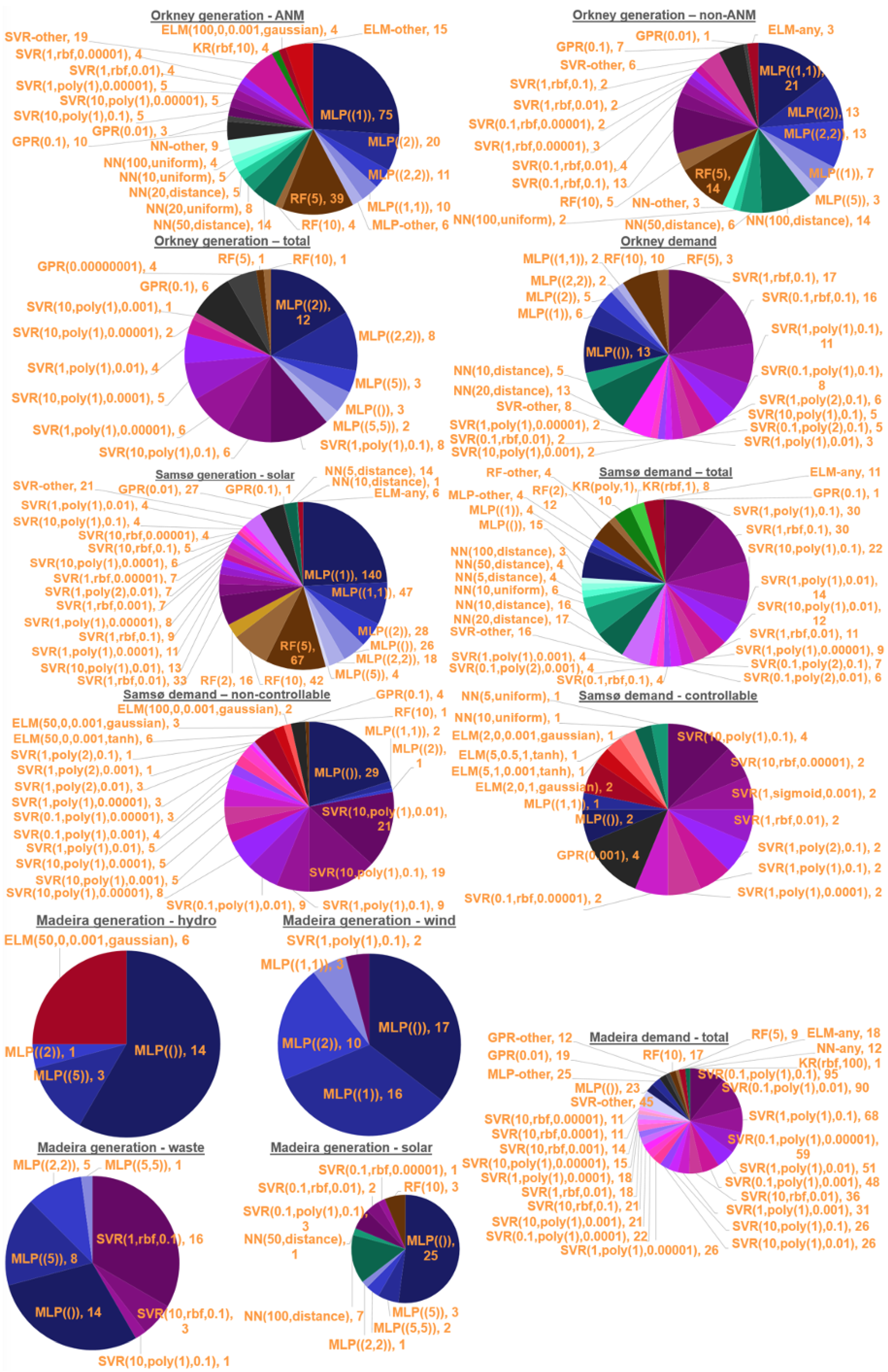
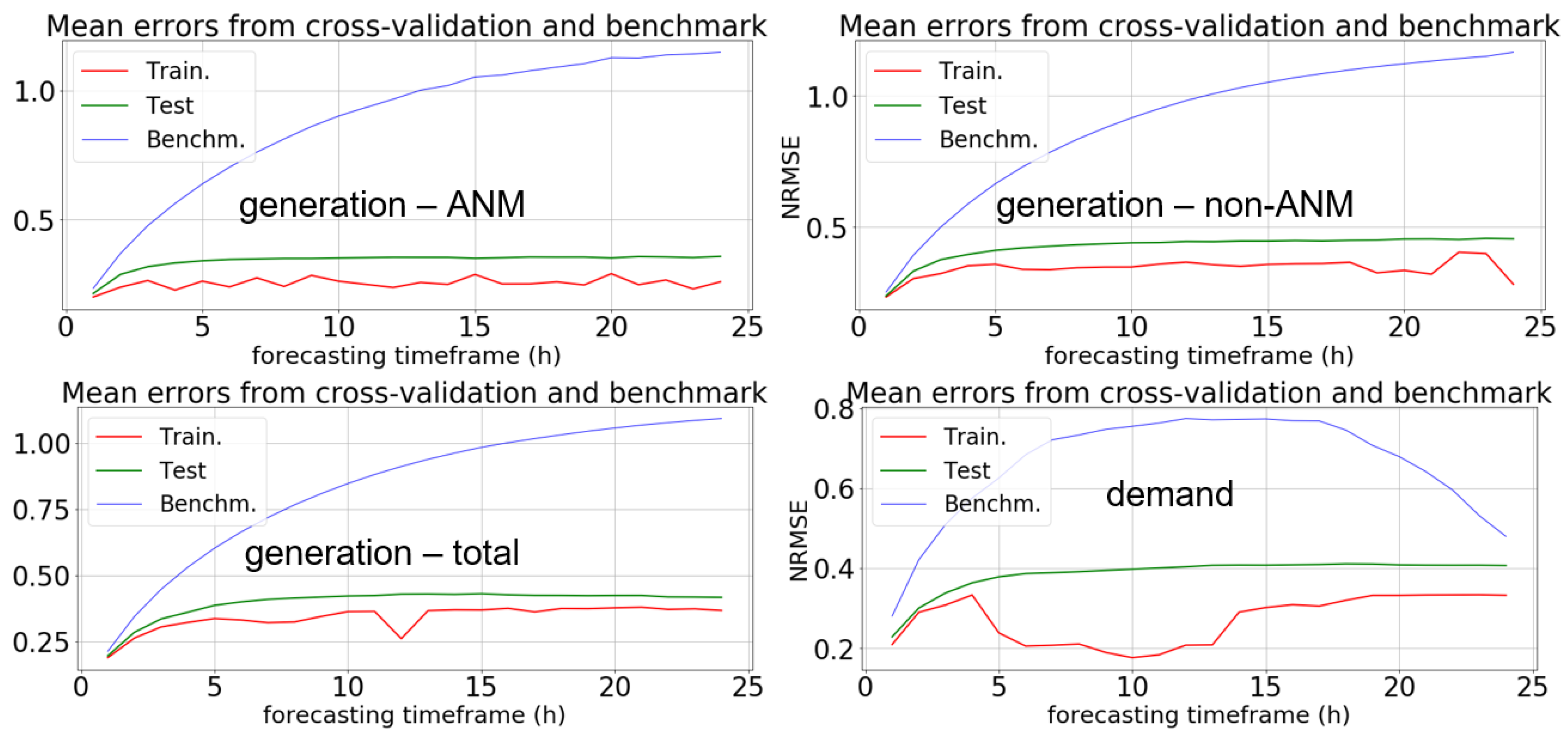
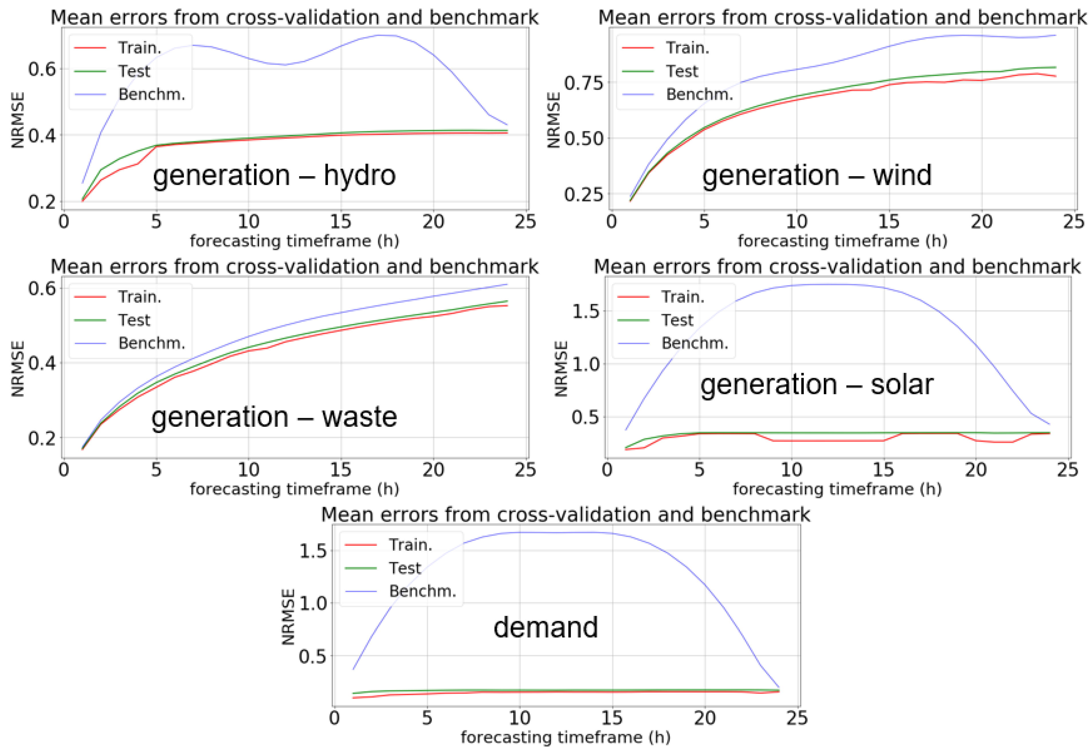
4.3.3. Results from Training the Regression Models
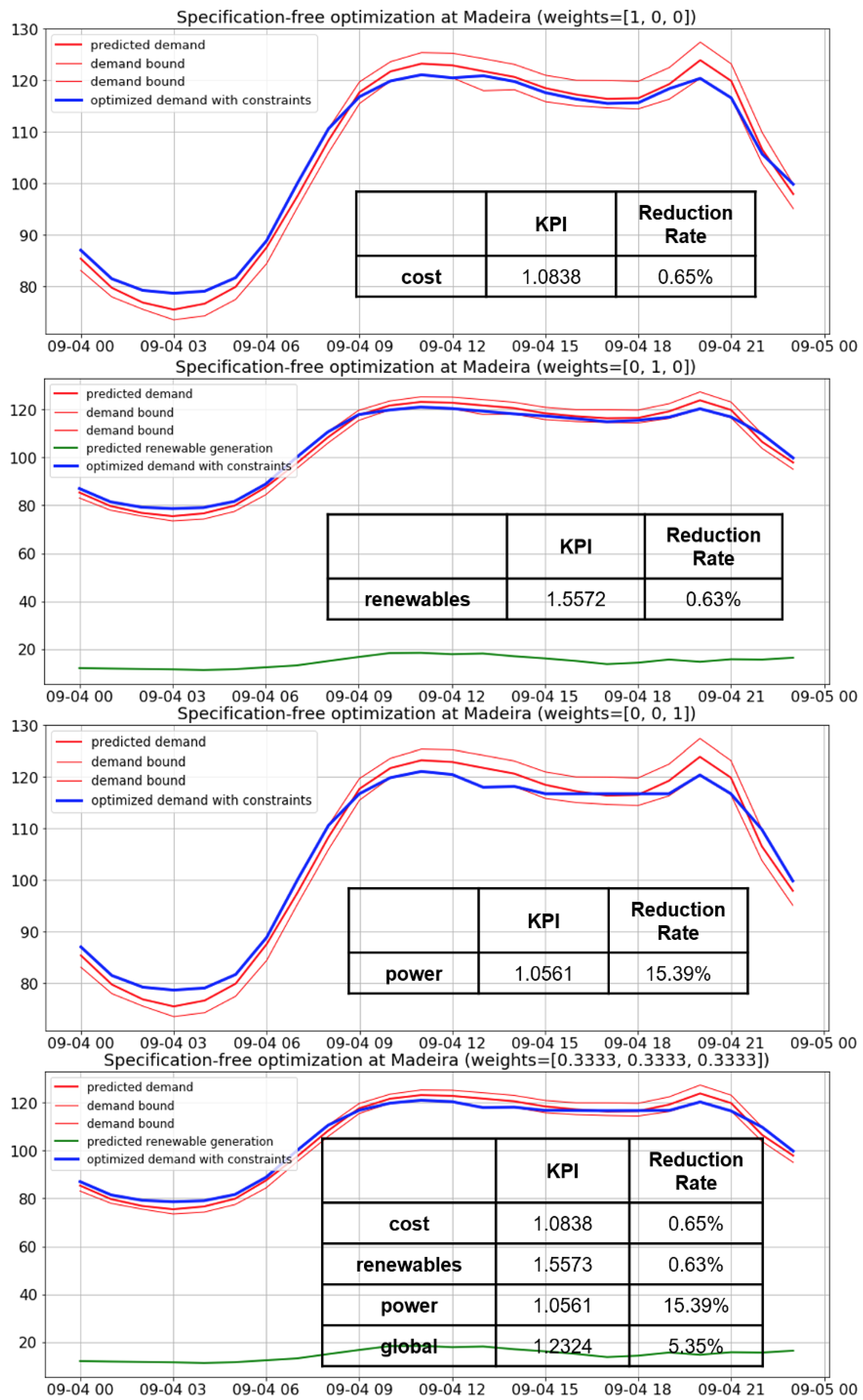
5. The Optimization Algorithm
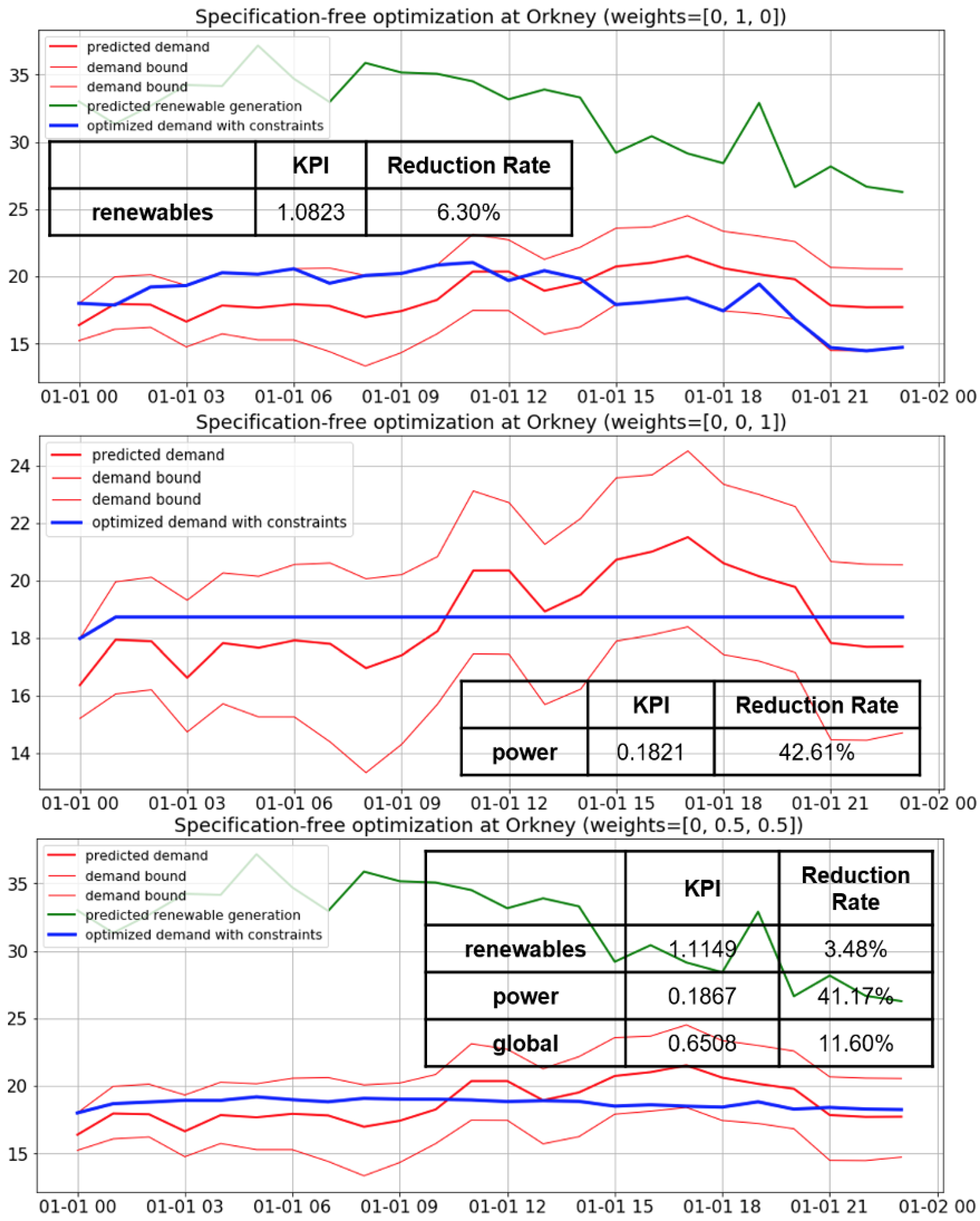
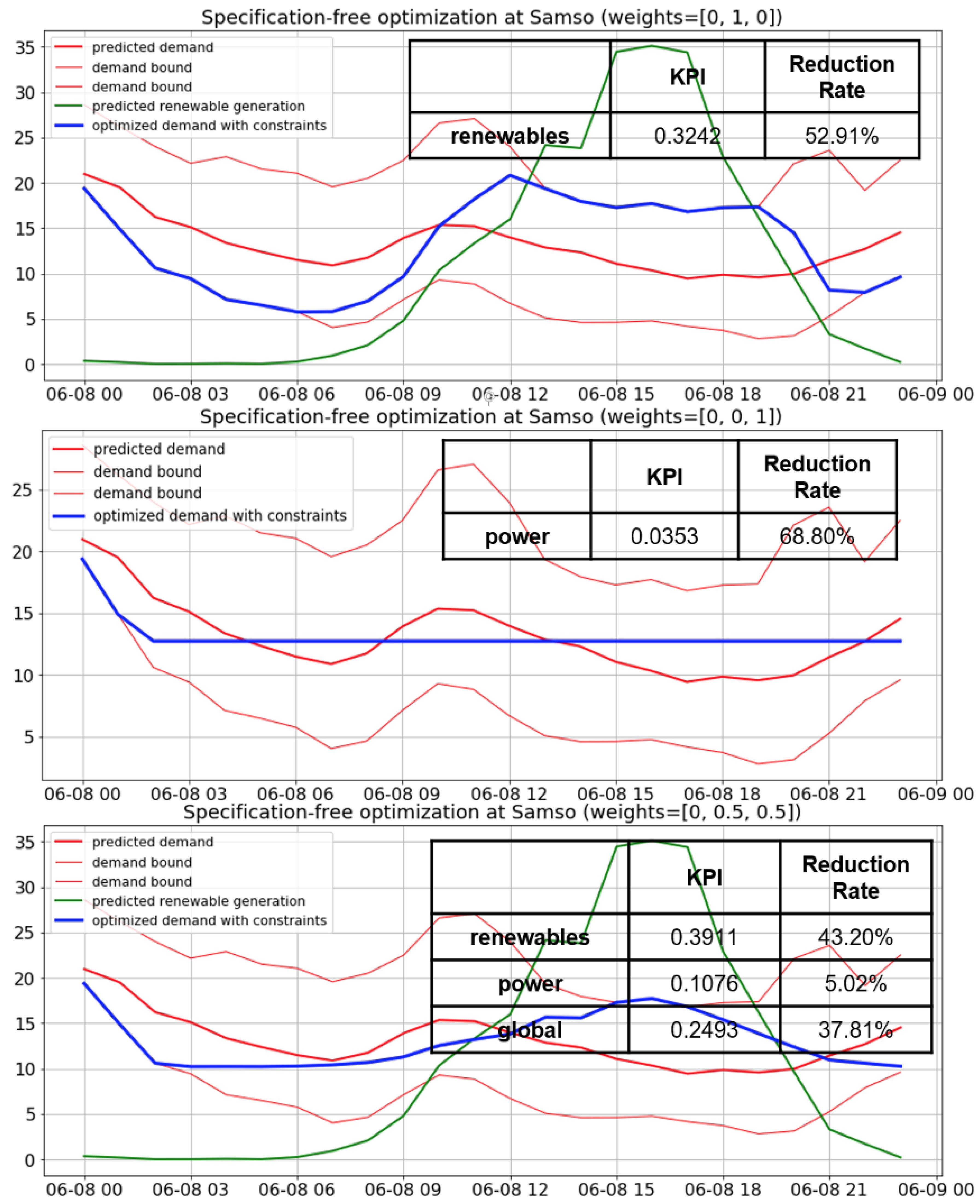
- minimum cost (minimum mean product of demand and price per energy unit of demand)
- maximum usage of renewable energy (minimum variance of difference between demand and forecast generation)
- minimum power instability (minimum demand variance)
- Within the optimization interval, the total demand equals the total forecast demand (w.r.t. time). This means that demand can only be shifted, but not reduced overall.
- At each time point of the optimization interval, demand is within a time-point-dependent interval.
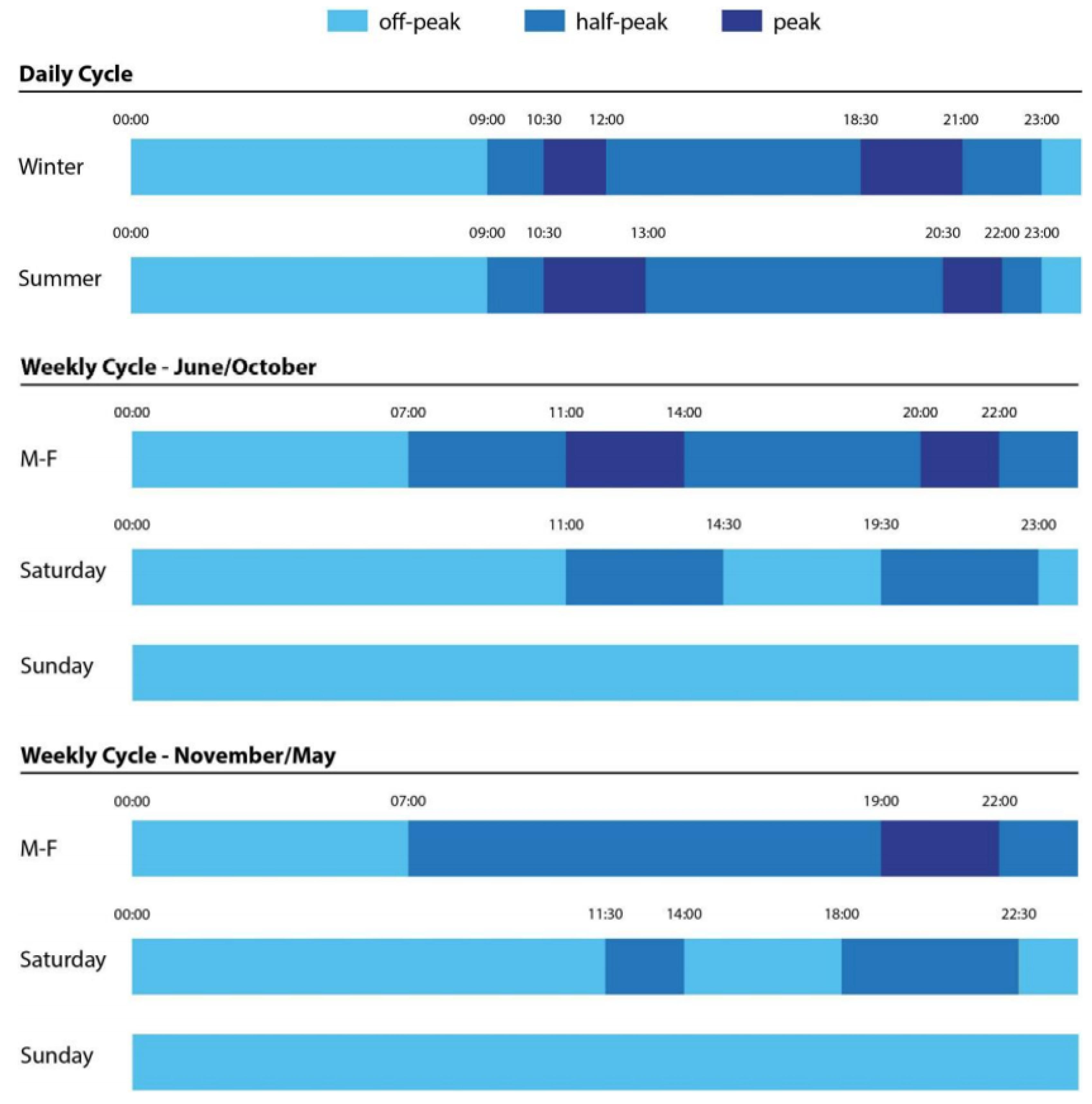
- peak: €0.1773/kWh
- half-peak: €0.1272/kWh
- off-peak: €0.0624/kWh
5.1. The Mathematical Viewpoint of the Optimization Method
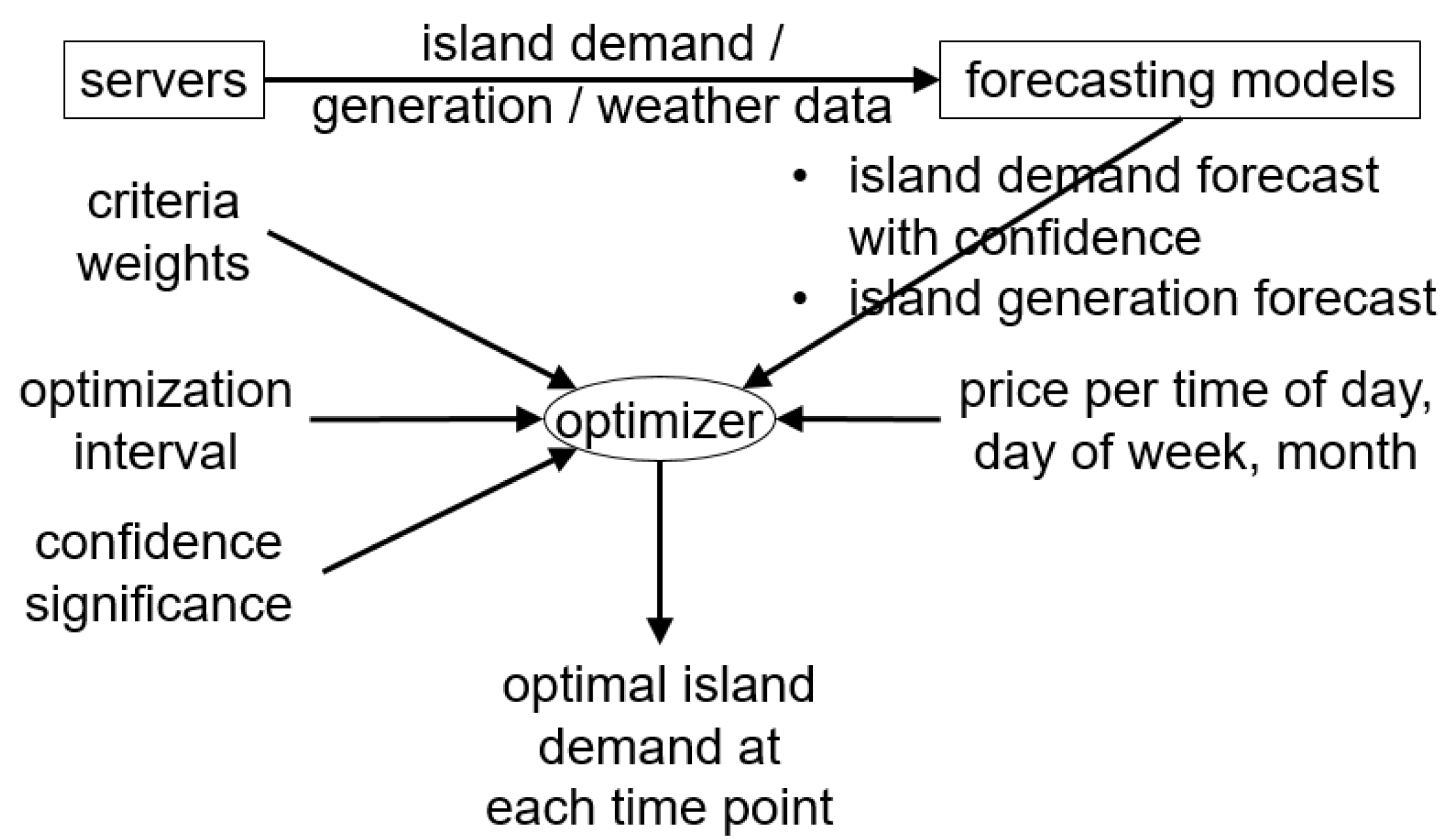
5.2. Methodology of the Optimization Algorithm
- optimization interval
- weighting coefficients of the optimization criteria
- aggregate demand forecast with confidence, based on a configurable significance level
- aggregate generation forecast (when the renewables-related criterion is considered)
- demand price at each time of the day, considering also day of week and month
- : interval for which the optimization takes place
- : aggregate demand (power) at time t
- : vector of all , , in ascending order of time
- : forecast aggregate demand at time t
- : 95% confidence interval for demand at time t (as explained in Section 4.1, the bounds depend on the predicted demand, but their difference from predicted demand depends only on the forecasting horizon, time of the day and clustering group)
- , , : KPIs for cost, renewables and power stability criteria respectively
- : arbitrary weights of KPIs
- : interval of training data for the demand forecasting models
- : expected aggregate demand cost per energy unit at the time point t (historical prices are set according to the same pricing policy of the current year)
- : aggregate generation at the time point t
- : theoretical variance of within (assuming mean as constant equal to the historical mean demand)
- : sample variance of within
5.3. Flexibility Analysis
- x: type of KPI (cost, renewables or power criterion, or combination)
- : reduction rate of within optimization interval
- : vector of forecast aggregate demand at all time points of in ascending order of time
- : vector of forecast optimal aggregate demand at all time points of in ascending order of time
5.4. Implementation Examples of the Optimization Algorithm and Discussion
6. Conclusions, Limitations and Future Work
Author Contributions
Funding
Institutional Review Board Statement
Informed Consent Statement
Data Availability Statement
Acknowledgments
Conflicts of Interest
Abbreviations
| AC | Agglomerative Clustering |
| AHP | analytical hierarchy process |
| ANM | Active Network Management |
| ANN | Artificial Neural Network |
| AP | Affinity Propagation |
| API | Application Programming Interface |
| ARFIMA | Autoregressive Fractionally Integrated Moving Average |
| ARIMA | Autoregressive Integrated Moving Average |
| ARMA | Autoregressive Moving Average |
| BATS | Box–Cox transformation, ARMA errors, Trend and Seasonal components |
| BESS | Battery Energy Storage System |
| CPP | Critical Peak Pricing |
| DR | Demand Response |
| ELM | Extreme Learning Machine |
| EPSO | Evolutionary Particle Swarm Optimization |
| EV | electric vehicle |
| GPR | Gaussian Process Regressor |
| GRBFN | Generalized Radial Basis Function Network |
| KM | K-Means |
| KPI | Key Performance Indicator |
| KR | Kernel Regression |
| MAUT | multi-attribute utility theory |
| MAVT | multi-attribute value theory |
| MCDA | multi-criteria decision analysis |
| MLP | Multi-Layer Perceptron |
| MS | Mean Shift |
| NN | Nearest Neighbour Regressor |
| NRMSE | Normalized Root Mean Square Error |
| PSO | Particle Swarm Optimization |
| PV | photovoltaic |
| QPSO | Quantum PSO |
| RBF | Radial Basis Function |
| RF | Random Forest Regressor |
| RTP | Real-Time Pricing |
| SARIMA | Seasonal Autoregressive Integrated Moving Average |
| SPEA | strength Pareto evolutionary algorithm |
| SVR | Support Vector Regressor |
| TOU | Time-of-Use |
| TS | Tabu search |
Appendix A. Access to Raw Data and Statistical Analysis

| Demonstrator | Output | Count | Mean | Standard Deviation | Minimum | Median | Maximum |
|---|---|---|---|---|---|---|---|
| Orkney | generation—ANM | 10,520 | 8.21 MW | 6.28 MW | 0.00 MW | 7.21 MW | 20.79 MW |
| generation—non-ANM | 10,440 | 11.16 MW | 6.59 MW | 0.19 MW | 11.90 MW | 26.04 MW | |
| generation—total (wind) | 11,061 | 18.34 MW | 12.68 MW | 0.00 MW | 17.98 MW | 42.78 MW | |
| demand | 11,060 | 16.99 MW | 3.99 MW | 2.68 MW | 17.22 MW | 33.75 MW | |
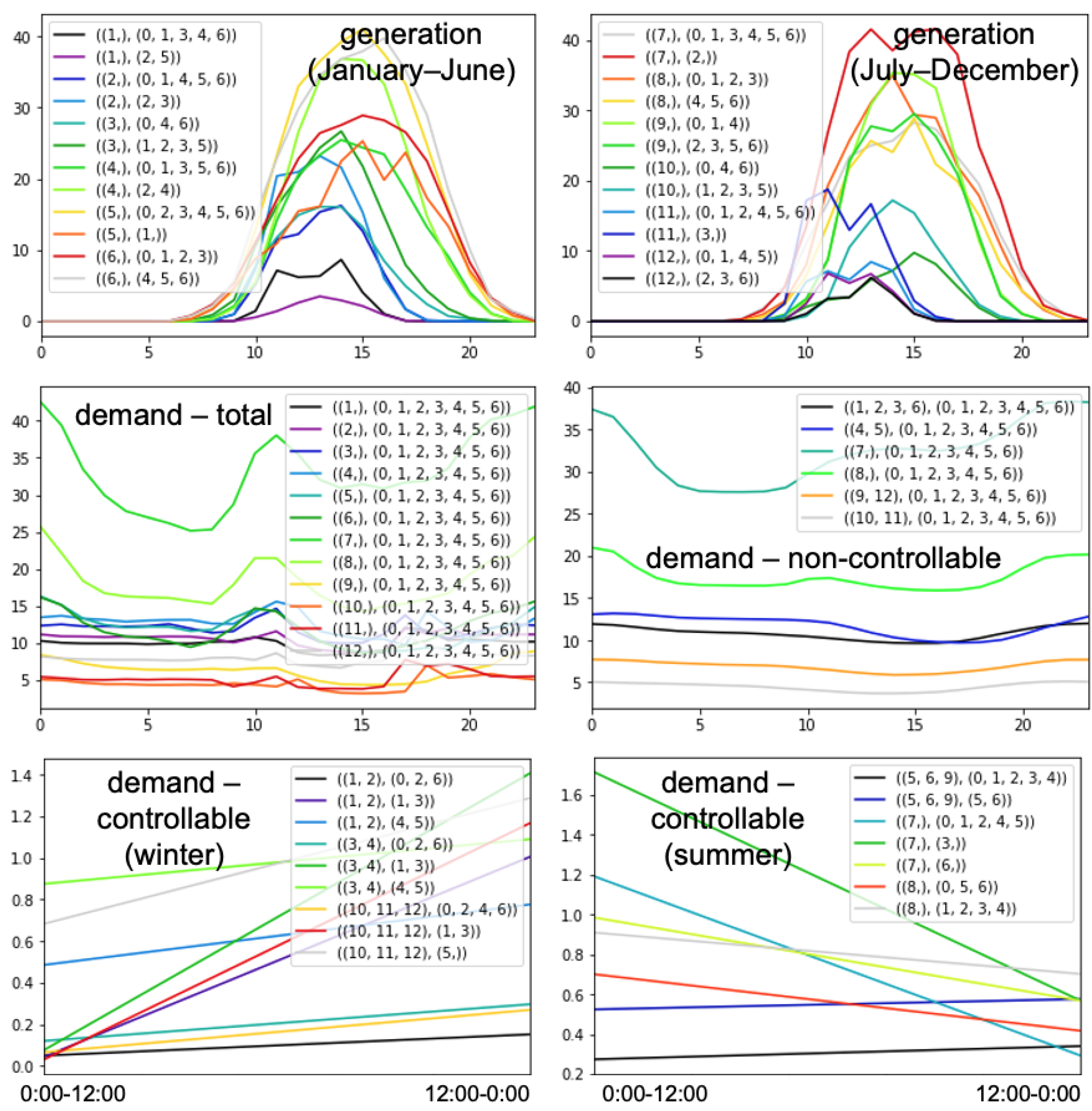
| Samsø | generation—solar | 8769 | 6.33 KW | 11.63 KW | 0.00 KW | 0.04 KW | 50.34 KW |
| demand—total | 9935 | 12.07 KW | 9.13 KW | 1.44 KW | 9.75 KW | 77.88 KW | |
| demand—non-controllable | 9937 | 11.62 KW | 8.57 KW | 1.68 KW | 9.60 KW | 67.20 KW | |
| demand—controllable | 828 | 0.47 KW | 0.54 KW | 0.00 KW | 0.23 KW | 3.02 KW | |
| Madeira | generation—hydro | 15,017 | 7.84 MW | 8.47 MW | 0.83 MW | 3.89 MW | 42.95 MW |
| generation—wind | 15,017 | 11.06 MW | 10.39 MW | 0.02 MW | 7.79 MW | 40.48 MW | |
| generation—waste | 15,017 | 4.22 MW | 1.83 MW | 0.00 MW | 4.90 MW | 6.68 MW | |
| generation—solar | 15,017 | 2.87 MW | 3.93 MW | 0.00 MW | 0.15 MW | 13.93 MW | |
| demand | 15,017 | 96.47 MW | 17.77 MW | 62.09 MW | 100.64 MW | 136.74 MW |


References
- Tealab, A. Time series forecasting using artificial neural networks methodologies: A systematic review. Future Comput. Inform. J. 2018, 3, 334–340. [Google Scholar] [CrossRef]
- Sagheer, A.; Kotb, M. Time series forecasting of petroleum production using deep LSTM recurrent networks. Neurocomputing 2019, 323, 203–213. [Google Scholar] [CrossRef]
- Weigend, A.S.; Gershenfeld, N.A. Time Series Prediction: Forecasting the Future and Understanding The Past; Routledge: New York, NY, USA, 2018. [Google Scholar]
- Papacharalampous, G.; Tyralis, H.; Koutsoyiannis, D. Predictability of monthly temperature and precipitation using automatic time series forecasting methods. Acta Geophys. 2018, 66, 807–831. [Google Scholar] [CrossRef]
- Wang, L.; Wang, Z.; Qu, H.; Liu, S. Optimal Forecast Combination Based on Neural Networks for Time Series Forecasting. Appl. Soft Comput. 2018, 66, 1–17. [Google Scholar] [CrossRef]
- McAlinn, K.; West, M. Dynamic Bayesian predictive synthesis in time series forecasting. J. Econ. 2019, 210, 155–169. [Google Scholar] [CrossRef]
- Singh, P.; Dhiman, G. A hybrid fuzzy time series forecasting model based on granular computing and bio-inspired optimization approaches. J. Comput. Sci. 2018, 27, 370–385. [Google Scholar] [CrossRef]
- Notton, G.; Nivet, M.-L.; Voyant, C.; Paoli, C.; Darras, C.; Motte, F.; Fouilloy, A. Intermittent and stochastic character of renewable energy sources: Consequences, cost of intermittence and benefit of forecasting. Renew. Sustain. Energy Rev. 2018, 87, 96–105. [Google Scholar] [CrossRef]
- Petrollese, M.; Cau, G.; Cocco, D. Use of weather forecast for increasing the self-consumption rate of home solar systems: An Italian case study. Appl. Energy 2018, 212, 746–758. [Google Scholar] [CrossRef]
- Veras, J.M.; Silva, I.R.S.; Pinheiro, P.R.; Rabêlo, R.A.L.; Veloso, A.F.S.; Borges, F.A.S.; Rodrigues, J.J.P.C. A Multi-Objective Demand Response Optimization Model for Scheduling Loads in a Home Energy Management System. Sensors 2018, 18, 3207. [Google Scholar] [CrossRef]
- Hu, M.; Xiao, J.-W.; Cui, S.-C.; Wang, Y.-W. Distributed real-time demand response for energy management scheduling in smart grid. Int. J. Electr. Power Energy Syst. 2018, 99, 233–245. [Google Scholar] [CrossRef]
- Available online: https://darksky.net/dev/docs (accessed on 19 May 2021).
- Yaseen, Z.M.; Allawi, M.F.; Yousif, A.A.; Jaafar, O.; Hamzah, F.M.; El-Shafie, A. Non-tuned machine learning approach for hydrological time series forecasting. Neural Comput. Appl. 2018, 30, 1479–1491. [Google Scholar] [CrossRef]
- Available online: https://www.next-kraftwerke.be/en/knowledge-hub/the-increasing-importance-of-flexibility/ (accessed on 19 May 2021).
- Xue, P.; Jiang, Y.; Zhou, Z.; Chen, X.; Fang, X.; Liu, J. Multi-step ahead forecasting of heat load in district heating systems using machine learning algorithms. Energy 2019, 188, 116085. [Google Scholar] [CrossRef]
- Van der Meer, D.W.; Widén, J.; Munkhammar, J. Review on probabilistic forecasting of photovoltaic power production and electricity consumption. Renew. Sustain. Energy Rev. 2018, 81, 1484–1512. [Google Scholar] [CrossRef]
- Hong, T.; Fan, S. Probabilistic electric load forecasting: A tutorial review. Int. J. Forecast. 2016, 32, 914–938. [Google Scholar] [CrossRef]
- Hong, T.; Pinson, P.; Fan, S.; Zareipour, H.; Troccoli, A.; Hyndman, R.J. Probabilistic energy forecasting: Global energy forecasting competition 2014 and beyond. Int. J. Forecast. 2016, 32, 896–913. [Google Scholar] [CrossRef]
- Gaillard, P.; Goude, Y.; Nedellec, R. Additive models and robust aggregation for GEFCom2014 probabilistic electric load and electricity price forecasting. Int. J. Forecast. 2016, 32, 1038–1050. [Google Scholar] [CrossRef]
- Van der Meer, D.W.; Shepero, M.; Svensson, A.; Widén, J.; Munkhammar, J. Probabilistic forecasting of electricity consumption, photovoltaic power generation and net demand of an individual building using Gaussian Processes. Appl. Energy 2018, 213, 195–207. [Google Scholar] [CrossRef]
- Hong, T.; Pinson, P.; Wang, Y.; Weron, R.; Yang, D.; Zareipour, H. Energy forecasting: A review and outlook. IEEE Open Access J. Power Energy 2020, 7, 376–388. [Google Scholar] [CrossRef]
- Ding, S.; Hipel, K.W.; Dang, Y. Forecasting China’s electricity consumption using a new grey prediction model. Energy 2018, 149, 314–328. [Google Scholar] [CrossRef]
- Ding, S. A novel self-adapting intelligent grey model for forecasting China’s natural-gas demand. Energy 2018, 162, 393–407. [Google Scholar] [CrossRef]
- De Oliveira, E.M.; Oliveira, F.L.C. Forecasting mid-long term electric energy consumption through bagging ARIMA and exponential smoothing methods. Energy 2018, 144, 776–788. [Google Scholar] [CrossRef]
- Gellert, A.; Florea, A.; Fiore, U.; Palmieri, F.; Zanetti, P. A study on forecasting electricity production and consumption in smart cities and factories. Int. J. Inf. Manag. 2019, 49, 546–556. [Google Scholar] [CrossRef]
- Rehman, A.; Deyuan, Z. Pakistan’s energy scenario: A forecast of commercial energy consumption and supply from different sources through 2030. Energy Sustain. Soc. 2018, 8, 26. [Google Scholar] [CrossRef]
- Mele, E.; Elias, C.; Ktena, A. Electricity use profiling and forecasting at microgrid level. In Proceedings of the IEEE 59th International Scientific Conference on Power and Electrical Engineering of Riga Technical University (RTUCON), Riga, Latvia, 12–13 November 2018; pp. 1–6. [Google Scholar]
- Elmouatamid, A.; Ouladsine, A.; Bakhouya, M.; El kamoun, N.; Zine-Dine, K.; Khaidar, M. A Control Strategy Based on Power Forecasting for Micro-Grid Systems. In Proceedings of the IEEE International Smart Cities Conference (ISC2), Casablanca, Morocco, 14–17 October 2019; pp. 735–740. [Google Scholar]
- Györi, A.; Niederau, M.; Zeller, V.; Stich, V. Evaluation of Deep Learning-based prediction models in Microgrids. In Proceedings of the IEEE Conference on Energy Conversion (CENCON), Yogyakarta, Indonesia, 16–17 October 2019; pp. 95–99. [Google Scholar]
- Akarslan, E.; Hocaoglu, F.O. Electricity demand forecasting of a micro grid using ANN. In Proceedings of the 9th International Renewable Energy Congress (IREC), Hammamet, Tunisia, 20–22 March 2018; pp. 1–5. [Google Scholar]
- Morais, H.; Vale, Z.A.; Soares, J.; Sousa, T.; Nara, K.; Theologi, A.M.; Rueda, J.; Ndreko, M.; Erlich, I.; Mishra, S.; et al. Integration of renewable energy in smart grid. In Applications of Modern Heuristic Optimization Methods in Power and Energy Systems; Lee, K.Y., Vale, Z.A., Eds.; Wiley-IEEE Press: Hoboken, NJ, USA, 2020; pp. 613–773. [Google Scholar]
- Rodríguez, F.; Fleetwood, A.; Galarza, A.; Fontán, L. Predicting solar energy generation through artificial neural networks using weather forecasts for microgrid control. Renew. Energy 2018, 126, 855–864. [Google Scholar] [CrossRef]
- Linkov, I.; Satterstrom, F.K.; Kiker, G.; Seager, T.P.; Bridges, T.; Gardner, K.H.; Rogers, S.H.; Belluck, D.A.; Meyer, A. Multicriteria Decision Analysis: A Comprehensive Decision Approach for Management of Contaminated Sediments. Risk Anal. 2006, 26, 61–78. [Google Scholar] [CrossRef] [PubMed]
- Stoycheva, S.; Marchese, D.; Paul, C.; Padoan, S.; Juhmani, A.; Linkov, I. Multi-criteria decision analysis framework for sustainable manufacturing in automotive industry. J. Clean. Prod. 2018, 187, 257–272. [Google Scholar] [CrossRef]
- Godina, R.; Rodrigues, E.M.G.; Pouresmaeil, E.; Matias, J.C.O.; Catalão, J.P.S. Model Predictive Control Home Energy Management and Optimization Strategy with Demand Response. Appl. Sci. 2018, 8, 408. [Google Scholar] [CrossRef]
- Gazijahani, F.S.; Salehi, J. Reliability constrained two-stage optimization of multiple renewable-based microgrids incorporating critical energy peak pricing demand response program using robust optimization approach. Energy 2018, 161, 999–1015. [Google Scholar] [CrossRef]
- Appino, R.R.; Ordiano, J.; Ordiano, J.Á.G.; Mikut, R.; Faulwasser, T.; Hagenmeyer, V. On the use of probabilistic forecasts in scheduling of renewable energy sources coupled to storages. Appl. Energy 2018, 210, 1207–1218. [Google Scholar] [CrossRef]
- Wang, Y.; Huang, Y.; Wang, Y.; Zeng, M.; Li, F.; Wang, Y.; Zhang, Y. Energy management of smart micro-grid with response loads and distributed generation considering demand response. J. Clean. Prod. 2018, 197, 1069–1083. [Google Scholar] [CrossRef]
- Wang, Y.; Huang, Y.; Wang, Y.; Li, F.; Zhang, Y.; Tian, C. Operation Optimization in a Smart Micro-Grid in the Presence of Distributed Generation and Demand Response. Sustainability 2018, 10, 847. [Google Scholar] [CrossRef]
- Liu, T.; Zhang, D.; Wang, S.; Wu, T. Standardized modelling and economic optimization of multi-carrier energy systems considering energy storage and demand response. Energy Convers. Manag. 2019, 182, 126–142. [Google Scholar] [CrossRef]
- Nojavan, S.; Nourollahi, R.; Pashaei-Didani, H.; Zare, K. Uncertainty-based electricity procurement by retailer using robust optimization approach in the presence of demand response exchange. Int. J. Electr. Power Energy Syst. 2019, 105, 237–248. [Google Scholar] [CrossRef]
- Xiong, Y.; Wang, B.; Chu, C.; Gadh, R. Vehicle grid integration for demand response with mixture user model and decentralized optimization. Appl. Energy 2018, 231, 481–493. [Google Scholar] [CrossRef]
- Neves, D.; Pina, A.; Silva, C.A. Comparison of different demand response optimization goals on an isolated microgrid. Sustain. Energy Technol. Assess. 2018, 30, 209–215. [Google Scholar] [CrossRef]
- Veras, J.M.; Silva, I.R.S.; Pinheiro, P.R.; Rabêlo, R.A.L. Towards the Handling Demand Response Optimization Model for Home Appliances. Sustainability 2018, 10, 616. [Google Scholar] [CrossRef]
- Carli, R.; Dotoli, M.; Jantzen, J.; Kristensen, M.; Othman, S.B. Energy scheduling of a smart microgrid with shared photovoltaic panels and storage: The case of the Ballen marina in Samsø. Energy 2020, 198, 117188. [Google Scholar] [CrossRef]
- Hashmi, M.U.; Pereira, L.; Bušić, A. Energy storage in Madeira, Portugal: Co-optimizing for arbitrage, self-sufficiency, peak shaving and energy backup. In Proceedings of the 2019 IEEE Milan PowerTech, Milan, Italy, 23–27 June 2019; pp. 1–6. [Google Scholar]
- Murphy, M.D.; O’Mahony, M.J.; Upton, J. Comparison of control systems for the optimisation of ice storage in a dynamic real time electricity pricing environment. Appl. Energy 2015, 149, 392–403. [Google Scholar] [CrossRef]
- Craparo, E.; Karatas, M.; Singham, D.I. A robust optimization approach to hybrid microgrid operation using ensemble weather forecasts. Appl. Energy 2017, 201, 135–147. [Google Scholar] [CrossRef]
- Mkireb, C.; Dembélxex, A.; Jouglet, A.; Denoeux, T. Robust Optimization of Demand Response Power Bids for Drinking Water Systems. Appl. Energy 2019, 238, 1036–1047. [Google Scholar] [CrossRef]
- Huang, W.; Zhang, N.; Kang, C.; Li, M.; Huo, M. From demand response to integrated demand response: Review and prospect of research and application. Prot. Control Modern Power Syst. 2019, 4, 12. [Google Scholar] [CrossRef]
- Rakipour, D.; Barati, H. Probabilistic optimization in operation of energy hub with participation of renewable energy resources and demand response. Energy 2019, 173, 384–399. [Google Scholar] [CrossRef]
- Golmohamadi, H.; Keypour, R.; Bak-Jensen, B.; Pillai, J.R. A multi-agent based optimization of residential and industrial demand response aggregators. Int. J. Electr. Power Energy Syst. 2019, 107, 472–485. [Google Scholar] [CrossRef]
- Otashu, J.I.; Baldea, M. Demand response-oriented dynamic modeling and operational optimization of membrane-based chlor-alkali plants. Comput. Chem. Eng. 2019, 121, 396–408. [Google Scholar] [CrossRef]
- Jahani, M.A.T.G.; Nazarian, P.; Safari, A.; Haghifam, M.R. Multi-objective optimization model for optimal reconfiguration of distribution networks with demand response services. Sustain. Cities Soc. 2019, 47, 101514. [Google Scholar] [CrossRef]
- Hassan, M.A.S.; Chen, M.; Lin, H.; Ahmed, M.H.; Khan, M.Z.; Chughtai, G.R. Optimization modeling for dynamic price based demand response in microgrids. J. Clean. Prod. 2019, 222, 231–241. [Google Scholar] [CrossRef]
- Available online: https://scikit-learn.org/stable/ (accessed on 19 May 2021).
- Available online: https://pypi.org/project/sklearn-extensions/ (accessed on 19 May 2021).
- Available online: https://www.scribd.com/document/451430756/Attachment-0 (accessed on 19 May 2021).
- Available online: https://docs.scipy.org/doc/scipy/reference/generated/scipy.optimize.basinhopping.html (accessed on 19 May 2021).
- Available online: https://github.com/nikolokas/paper-power-forecasting-optimization (accessed on 19 May 2021).
- Zyglakis, L.; Zikos, S.; Kitsikoudis, K.; Bintoudi, A.D.; Tsolakis, A.C.; Ioannidis, D.; Tzovaras, D. Greek Smart House Nanogrid Dataset. Available online: https://zenodo.org/record/4246525#.X8oazBaxU1k (accessed on 19 May 2021).
- Tsolakis, A.C.; Bintoudi, A.D.; Zyglakis, L.; Zikos, S.; Timplalexis, C.; Bezas, N.; Kitsikoudis, K.; Ioannidis, D.; Tzovaras, D. Design and Real-Life Deployment of a Smart Nanogrid: A Greek Case Study. In Proceedings of the IEEE International Conference on Power and Energy (PECon), Penang, Malaysia, 7–8 December 2020. [Google Scholar]
- Salamanis, A.I.; Xanthopoulou, G.; Bezas, N.; Timplalexis, C.; Bintoudi, A.D.; Zyglakis, L.; Tsolakis, A.C.; Ioannidis, D.; Kehagias, D.; Tzovaras, D. Benchmark Comparison of Analytical, Data-Based and Hybrid Models for Multi-Step Short-Term Photovoltaic Power Generation Forecasting. Energies 2020, 13, 5978. [Google Scholar] [CrossRef]
- Tsolakis, A.C.; Kalamaras, I.; Vafeiadis, T.; Zyglakis, L.; Bintoudi, A.D.; Chouliara, A.; Ioannidis, D.; Tzovaras, D. Towards a Holistic Microgrid Performance Framework and a Data-Driven Assessment Analysis. Energies 2020, 13, 5780. [Google Scholar] [CrossRef]


| Demonstrator | Demand | Generation |
|---|---|---|
| Orkney | total (3 December 2018–6 April 2020) | wind ≃ total (ANM, non-ANM) (3 December 2018–6 April 2020) |
| Samsø | harbour (1 May 2016–19 June 2017) | PV estimation—harbour (2016) |
| Madeira | total (1 January 2018–30 November 2019) | hydro, wind, waste (“bio”), solar (1 January 2018–November 2019) |
| Demonstrator | Output | Input | Clustering Algorithms for Month/Day of Week | Month Groups & Respective Day of Week Groups (Sets) on the Left & Right Respectively of Slashes and Colons [Days are Numbered from 0 (Monday) to 6 (Sunday)] |
|---|---|---|---|---|
| Orkney | generation—ANM | present value, average time profile, wind speed, wind gust | singletons/- | singletons/- |
| generation—non-ANM | present value, wind speed, wind gust | KM(6)/- | {{10,1}, {11,12,2–4}, {5}, {6}, {7,8}, {9}}/- | |
| generation—total (wind) | present value, past values (≤23 h), wind speed, wind gust | MS/- | {{9–4}, {5}, {6–8}}/- | |
| demand | present value, past values (≤23 h), apparent temperature | KM(6)/- | {{11–2}, {3}, {4}, {5,10}, {6,9}, {7,8}}/- | |
| Samsø | generation—solar | present value, last value at same time, past values (1 h), average time profile, sun, humidity | singletons/KM(2) | {{1}:{{6–1,3,4},{2,5}}, {2}:{{4–1},{2,3}}, {3}:{{0,4,6},{1–3,5}}, {4}:{{5–1,3},{2,4}}, {5}:{{2–0},{1}}, {6}:{{0–3},{4–6}}, {7}:{{3–1},{2}}, {8}:{{0–3},{4–6}}, {9}:{{0,1,4},{2,3,5,6}}, {10}:{{0,4,6},{1–3,5}}, {11}:{{4–2},{3}}, {12}:{{0,1,4,5},{2,3,6}}} |
| demand—total | present value, past values (≤23 h) | singletons/- | singletons/- | |
| demand—non-controllable | present value, past values (≤23 h), average time profile | KM(6)/- | {{1–3,6}, {4,5}, {7}, {8}, {9–11}, {12}}/- | |
| demand—controllable | last value at same time, average time profile | KM(6)/AP | {{1,2}:{{0,2,6},{1,3},{4,5}}, {3,4}:{{0,2,6},{1,3},{4,5}}, {5,6,9}:{{0–4},{5,6}}, {7}:{{0–2,4,5},{3},{6}}, {8}:{{5–0},{1–4}}, {10–12}:{{0,2,4,6},{1,3},{5}}}} | |
| Madeira | generation—hydro | present value, past values (≤23 h) | -/- | -/- |
| generation—wind | present value, past values (≤23 h), average time profile, wind speed | AC(2)/- | {{10,11,1–4}, {5–9,12}}/- | |
| generation—waste | present value, last value at same time, average time profile | KM(2)/- | {{12,1,3–8}, {9–11,2}}/- | |
| generation—solar | present value, last value at same time, past values (1 h), average time profile, sun, humidity | KM(2)/- | {{10–2}, {3–9}}/- | |
| demand | present value, last value at same time, average time profile | singletons/MS | {{1}:{{0–4},{5},{6}}, {2}:{{0–4},{5},{6}}, {3}:{{0–4},{5},{6}}, {4}:{{0–4},{5},{6}}, {5}:{{0–4},{5},{6}}, {6}:{{0–4},{5},{6}}, {7}:{{0–4},{5},{6}}, {8}:{{0–4},{5},{6}}, {9}:{{0–4},{5},{6}}, {10}:{{0–4},{5},{6}}, {11}:{{0–4},{5},{6}}, {12}:{{0,3,4},{1,2},{5},{6}} |
| Demonstrator | Output | Proposed Approach | No Clustering—All Candidate Regressors | Same Clusters—Linear Regression | Same Clusters—Benchmark Regressor |
|---|---|---|---|---|---|
| Orkney | generation—ANM | 0.3419 | 0.4164 | 0.4283 | 0.9217 |
| generation—non-ANM | 0.4282 | 0.4727 | 0.5725 | 0.9351 | |
| generation—total (wind) | 0.4022 | 0.4300 | 0.4877 | 0.8715 | |
| demand | 0.3879 | 0.4141 | 0.4087 | 0.6715 | |
| Samsø | generation—solar | 0.3678 | 0.4360 | 0.4335 | 1.3081 |
| demand—total | 0.4108 | 0.4379 | 0.4209 | 0.5649 | |
| demand—non-controllable | 0.3112 | 0.3263 | 0.3206 | 0.3959 | |
| demand—controllable | 0.7122 | 0.9668 | 0.8152 | not computed | |
| Madeira | generation—hydro | 0.3846 | 0.3846 | 0.3855 | 0.6025 |
| generation—wind | 0.6862 | 0.6994 | 0.6880 | 0.8171 | |
| generation—waste | 0.4524 | 0.4534 | 0.4567 | 0.4852 | |
| generation—solar | 0.3371 | 0.3440 | 0.3396 | 1.3826 | |
| demand | 0.1674 | 0.2781 | 0.1846 | 1.3447 |
| Demonstrator | Cost | Renewables | Power |
|---|---|---|---|
| Orkney | not considered | 12.9285 MW | 3.9921 MW |
| Samsø | not considered | 16.8783 KW | 9.1264 KW |
| Madeira | 266,180/day | 73.5026 MW | 17.7684 MW |
Publisher’s Note: MDPI stays neutral with regard to jurisdictional claims in published maps and institutional affiliations. |
© 2021 by the authors. Licensee MDPI, Basel, Switzerland. This article is an open access article distributed under the terms and conditions of the Creative Commons Attribution (CC BY) license (https://creativecommons.org/licenses/by/4.0/).
Share and Cite
Kolokas, N.; Ioannidis, D.; Tzovaras, D. Multi-Step Energy Demand and Generation Forecasting with Confidence Used for Specification-Free Aggregate Demand Optimization. Energies 2021, 14, 3162. https://doi.org/10.3390/en14113162
Kolokas N, Ioannidis D, Tzovaras D. Multi-Step Energy Demand and Generation Forecasting with Confidence Used for Specification-Free Aggregate Demand Optimization. Energies. 2021; 14(11):3162. https://doi.org/10.3390/en14113162
Chicago/Turabian StyleKolokas, Nikolaos, Dimosthenis Ioannidis, and Dimitrios Tzovaras. 2021. "Multi-Step Energy Demand and Generation Forecasting with Confidence Used for Specification-Free Aggregate Demand Optimization" Energies 14, no. 11: 3162. https://doi.org/10.3390/en14113162
APA StyleKolokas, N., Ioannidis, D., & Tzovaras, D. (2021). Multi-Step Energy Demand and Generation Forecasting with Confidence Used for Specification-Free Aggregate Demand Optimization. Energies, 14(11), 3162. https://doi.org/10.3390/en14113162