Article

The Impact of Time Delays for Power Hardware-in-the-Loop Investigations

1
Institute for Mechatronics in Mechanics, Hamburg University of Technology, 21073 Hamburg, Germany
2
Institute of Electrical Power and Energy Technology, Hamburg University of Technology, 21079 Hamburg, Germany
*
Author to whom correspondence should be addressed.
Energies 2021, 14(11), 3154; https://doi.org/10.3390/en14113154
Submission received: 20 April 2021 / Revised: 20 May 2021 / Accepted: 25 May 2021 / Published: 28 May 2021
(This article belongs to the Section F: Electrical Engineering)

Abstract

:
Power hardware-in-the-loop (PHiL) simulations provide a powerful environment in the critical process of testing new components and controllers. In this work, we aim to explain the impact of time delays in a PHiL setup and recommend how to consider them in different investigations. The general concept of PHiL, with its necessary components, is explained and the benefits compared to pure simulation and implemented field tests are presented. An example for a flexible PHiL environment is shown in form of the Power Hardware-in-the-Loop Simulation Laboratory (PHiLsLab) at TU Hamburg. In the PHiLsLab, different hardware components are used as the simulator to provide a grid interface via an amplifier system, a real-time simulator by OPAL-RT, a programmable logic controller by Bachmann, and an M-DUINO microcontroller. Benefits and limitations of the different simulators are shown using case examples of conducted investigations. Essentially, all platforms prove to be appropriate and sufficiently powerful simulators, if the time constants and complexity of the investigated case fit the simulator performance. The communication interfaces used between simulator and amplifier system differ in communication speed and delay; therefore, they have to be considered to determine the level of dynamic interactions between the simulated rest of system and the hardware under test.

1. Introduction

Electric power grids are becoming increasingly complex due to rising shares of renewable energy systems, a growing number of DC loads, and changing generator characteristics [1]. Additionally, the transition of the power grid toward a smart grid is inducing major changes, especially with the rising integration of information and communication technology [2]. Since field tests are challenging to implement, simulations, controller hardware-in-the-loop (CHiL), or power hardware-in-the-loop (PHiL) applications are a viable approach for the validation of new power and energy system solutions.
New components and controllers that can be used in a future grid need to be tested under realistic conditions before integration into the power grid to prevent costly and dangerous failures. Direct dynamic testing of the hardware is often not possible because critical test cases occur randomly and rarely. Furthermore, direct testing might be impossible if future developments of the grid that do not yet exist have to be tested [3]. Moreover, high costs, space limitations, and potentially dangerous test conditions such as those of fault scenarios prevent such complete hardware applications; consequently, pure simulations, CHiL, or PHiL simulations are used. Pure simulations require high accuracy of the models, which results in long computing times [4]. In addition, the models’ limitations may alter the results or critical dynamics are missing due to simplification of the models [5]. As an alternative solution, CHiL and PHiL offer the possibility to combine the accuracy of hardware tests with the reproducibility of simulations.
CHiL models connect the simulation of the grid via low-power signals with the hardware under test (HUT), whereas high-power signals are used in a PHiL model. A PHiL model is thus the closest to a complete hardware application. It also allows to simulate different communication networks that can be used for control purposes. The transmission speed between the components of the PHiL laboratory influences the system dynamics because the real-time simulation works with fixed-time-step solvers and all parts of the PHiL system can potentially add further time delays. The delays of the individual components can reduce precision, cause instabilities, or even damage the equipment [5]. The matching time delays of the simulator and the amplifier are therefore essential and need to be selected according to the investigation. In particular, for the investigation of frequency deviations in the range of seconds, time delays in the range of milliseconds are adequate, whereas for other investigations, lower time delays may be needed. Depending on the necessary time step, high-, middle-, or low-end simulation hardware can be chosen.
Therefore, time delays and communication interfaces are of great importance for research using PHiL modeling. The goal of this work is to enable further research by giving an overview of different components that can be used in a PHiL setup. Different kinds of simulators are compared regarding performance and PHiL capabilities. In comparison to most current research activities, low-performance devices are used as simulators to show their potential in a PHiL setup.
The role of different simulators in power hardware-in-the-loop modeling is discussed in the upcoming sections and the advantages and disadvantages of different communication interfaces are explained. In Section 2, the different devices that are used for the investigation of power systems in PHiL are presented. The TU Hamburg laboratory setup is presented in Section 3, followed by three case examples, which are discussed in terms of communication and time delays in Section 4. A conclusion is provided in Section 5.

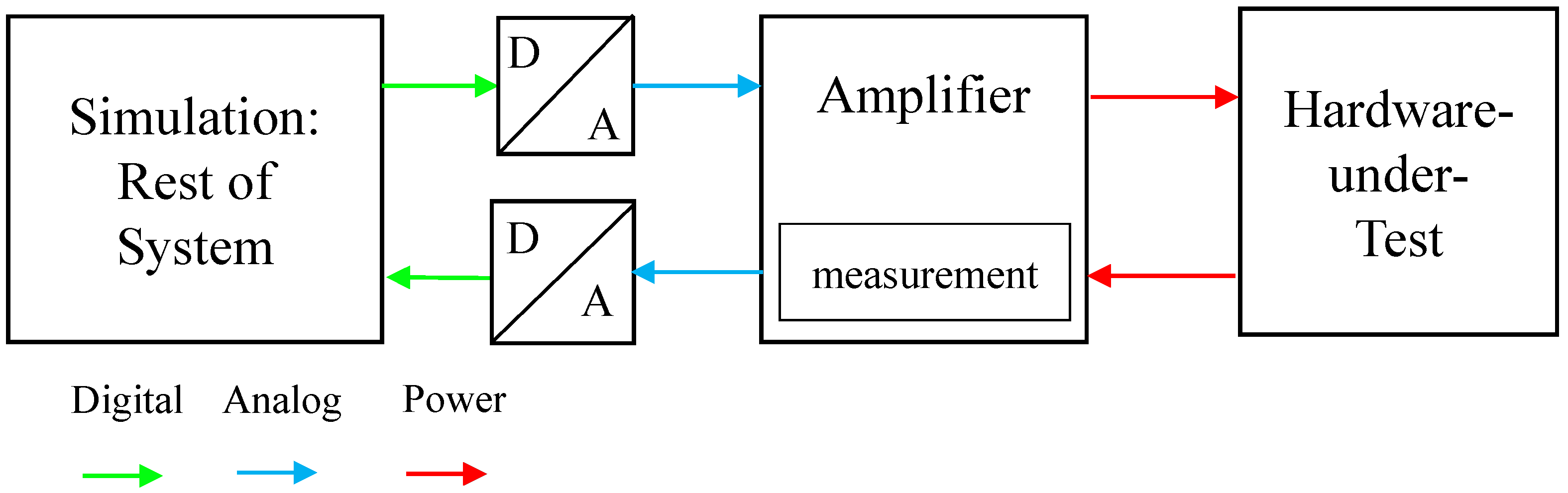
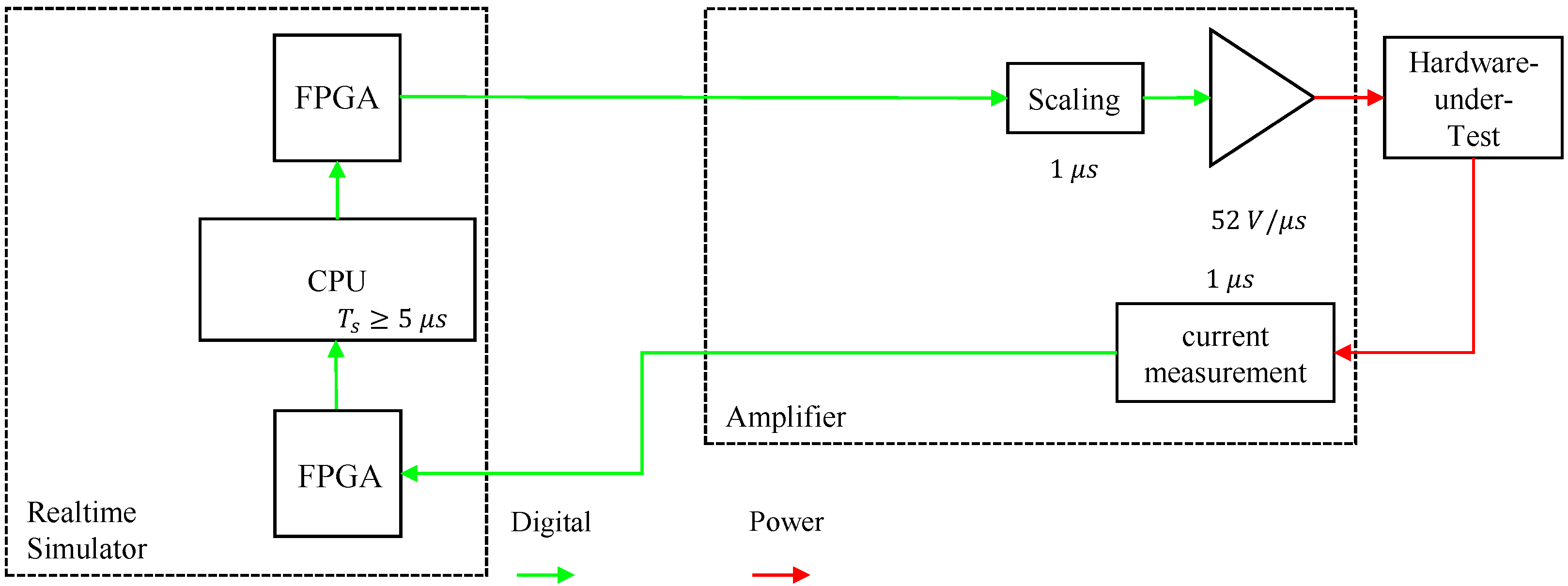
2. PHiL Device Overview

A PHiL laboratory evaluates the HUT that is connected to a simulation of the rest of system (ROS). Since high-power signals are used in PHiL setups, the signal from the simulator has to be amplified, usually by a power amplifier. The general setup of a PHiL simulation is shown in Figure 1.

2.1. Simulator

The simulation is a viable part of each CHiL and PHiL system and run on a real-time simulator (RTS). It is used to simulate the ROS, which contains physical or mathematical simulations of the surrounding system. Moreover, the simulator needs to offer a connection to a user interface and work with fixed time steps. A multitude of devices can be used as simulators; a real-time simulator and a programmable logic controller (PLC) are presented subsequently.

2.1.1. Real-Time Simulator

Depending on the dynamics of the model, the simulation in an RTS is either CPU-based or field-programmable-gate-array (FPGA)-based. A CPU simulation allows for more complex systems, but the simulation time step is limited to 5–10 μs depending on the hardware. A FPGA-based simulation allows for lower time steps and therefore a higher dynamic of the simulated systems. Due to the limited computational capacity of FPGAs, the simulated systems have to be smaller [6,7].

2.1.2. Programmable Logic Controller

A PLC is a modular system that employs different inputs and outputs as well as their programmable functional dependence. All measured data can be received and processed with the PLC and then the control signals can be communicated to the other devices. During operation, the PLC is running in cyclic operation and for every time step, an image table that describes all states of the inputs and outputs at this time is made. These image tables are only changed before and after each program cycle. A change of the outputs can therefore only be applied at the end of the program run, whereas a change of the input can only influence the next cycle. The time step can vary with the model complexity. Additionally, some PLCs allow visualization and diagnostics on a Web server that is run on the PLC [8,9].

2.2. Power Amplifier

The power amplifier serves as a connection between the simulation HUT by converting low voltage signals and frequency values from the simulation into physical quantities in real-time and vice versa.
A real system, which is actually stable, can become unstable by inserting an additional control loop between the ROS and the HUT. An ideal power amplifier would have zero time delay and infinite bandwidth, but its real dynamic behavior differs. Furthermore, quantization errors can have a fundamental role in PHiL simulation [4]. Additionally, the time delays of the ROS, measurements, and those of the simulated system itself occur and can lead to severe instabilities. However, possible instabilities that do not become evident in the HUT if used in real applications can occur in power hardware-in-the-loop simulations [10,11,12]. This nonideal behavior has to be tackled by the interface algorithm between the simulated system and the HUT [13]. Three options for power amplifiers have been used in PHiL setups with linear amplifiers, synchronous generators with load banks, and switched mode amplifiers. The switched mode amplifiers are composed of a rectifier, an inverter, and IGBT bridges and offer high power [10,11,14]. Whereas this type of amplifier induces a higher time delay and has a lower accuracy than other amplifiers [10,11,14], a linear amplifier possesses dynamic behavior with high accuracy and small time delays and therefore less stability issues [10,12]. In comparison to switched mode amplifiers, the achievable power ratings are lower. Using synchronous generators that are coupled to a DC motor and a thyristor drive is beneficial if a balanced three phase supply is necessary [10,15]. Ultimately, accuracy and power have to fit the intended use [16] to be able to test at a realistic power rating.

2.3. Hardware under Test

The HUT is connected with the power amplifier, which reproduces the simulated conditions at the HUT. Measured quantities from the HUT are then fed back to the simulation, which reacts to the measurement. Most signals transmitted between different devices can either be part of the test system or part of the HUT itself.
If the signal is part of the HUT, all delays induced by it are part of the tested hardware and therefore would also occur when the HUT is deployed in its intended application. An example is the communication between a battery system and the battery controller. In this case, communication is part of the test and does not need to be included in planning and building the test setup.
If the signal is part of the test setup instead, e.g., the communication between the RTS and the amplifier, the communication delay has to be considered for a stable and accurate test setup.

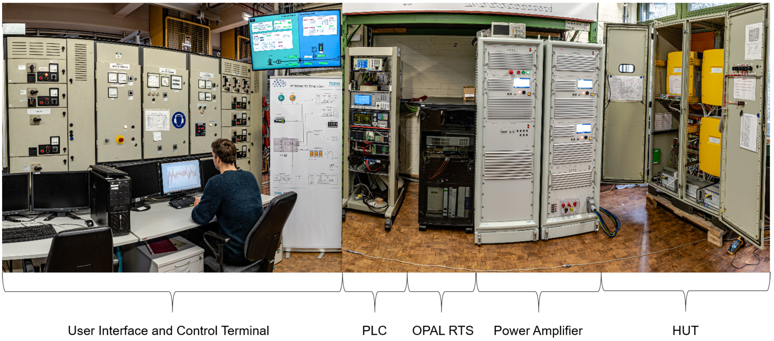
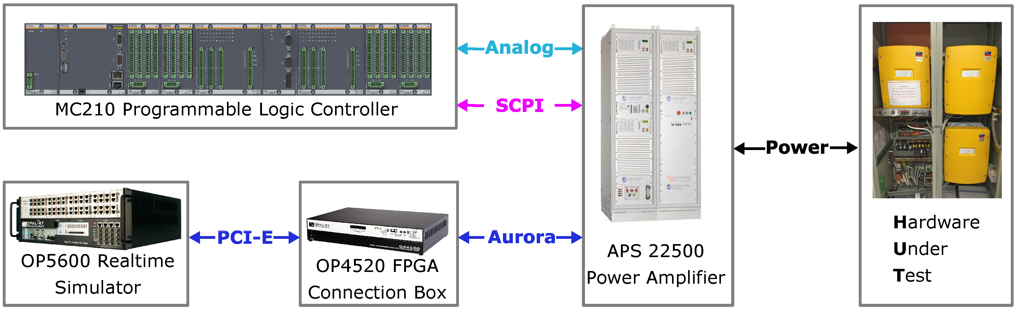
3. TU Hamburg Laboratory Setup—PHiLsLab

The PHiL system presented here is part of the Power Hardware-in-the-Loop Simulation Laboratory (PHiLsLab) at TU Hamburg depicted in Figure 2 and is designed especially for the investigation of three-phase island grids/microgrids with photovoltaic generators and battery energy storage systems (BESS) as well as ancillary service applications. Security mechanisms in both software and hardware such as software limits, fuses, and emergency stop switches were adopted to avoid damages to the laboratory setup or people.
Different techniques were employed to implement a PHiL setup using the available hardware. The general setup is shown in Figure 3. A simulator, either a PLC or an RTS, is connected to the amplifier using the available communication protocols. The connection is used to transmit set points and receive measurements from the amplifier. Power is exchanged between the amplifier and the HUT. Depending on the investigation, the amplifier can either be used in voltage or current control mode. In voltage control mode, a voltage set point is sent from the simulator and the current from or to the HUT results, vice versa in current control mode.

3.1. Three-Phased Power Amplifier System

The PHiLsLab uses a linear power amplifier by Spitzenberger & Spies for all of its PHiL setups. The system contains of three individual APS 7500 amplifiers [17] which work in source as well as in sink mode. In sink mode, it operates to one third of nominal power or with nominal power if a controlled load resistor, which can be operated by the amplifier without further software, is connected. The linear amplifier used at PHiLsLAB enables current and voltage limiting and has low harmonic distortions. It can supply voltages of up to 270 V rms in AC and 425 V in DC operation and can generate a variety of voltages and currents but is mainly used for sinusoidal voltages. Each of the three individual amplifiers can supply a power of 7.5 kW, making a total of 22.5 kw available. In order to be able to map requirements of high-frequency investigations and effects such as harmonics, a high bandwidth of up to 30 kHz was selected [17].
The power amplifier provides the necessary voltage/currents to the HUT and measures the resulting power flow. Depending on the communication between the amplifier and the simulator, the resulting voltage or current is sent to the simulator or additional values such as the power or frequency can be transmitted.
The amplifier system can be used in three-phase or single-phase operation. To connect three-phase hardware to a suitable simulation, the individual amplifiers are controlled to form a three-phase grid. Due to the use of three individual amplifiers, it is possible to simulate unbalanced cases with different voltages or a phase shift between lines as well as single line failures.
If only single phase hardware is tested, the amplifiers can be connected in parallel to increase the maximum current and therefore the maximum output power to the HUT. In single-phase operation, the amplifier can also be used to emulate DC grids.
The Spitzenberger & Spies power amplifier is able to receive and transmit signals via optical or analog communication or by using the Standard Commands for Programmable Instruments (SCPI). The different setups are explored in Section 4.

3.2. Simulator

The PHiLsLAB has two devices that are used as simulators. There is a PLC by Bachmann (MC210 [18]) and an OPAL-RT OP5600 RTS [19]. Both simulators work with fixed-time-step simulations, which is a necessary feature for PHiL investigations.
The Bachmann MC210 PLC has an ATOM E680 CPU with a frequency of 1.6 GHz. Models are created using MATLAB/Simulink® [20] and the dedicated Bachmann MTarget toolbox, which compiles the MATLAB/Simulink® model in C-code. The CPU module allows for time steps down to 200 μs. The PLC is able to communicate with the power amplifier using either analog communication or SCPI, which is also used for communication with measurement devices [8].
The OPAL-RT OP5600 uses an Intel Xenon E5V3 processor with eight cores running at 3.2 GHz. Models are created in MATLAB/Simulink® as well. The RTS is used for CPU simulations, which allow time steps down to 10 μs. The communication between the RTS and other devices can be implemented using analog signals or optical fiber connected to small form-factor pluggable ports.
Both simulators can be connected to the Spitzenberger & Spies power amplifier in multiple ways. For the PLC, an analog connection as well as a connection via SCPI is established. For the RTS, only the connection via optical fiber is used, since it is clearly advantageous over the analog connection if the used amplifier and simulator are supporting it.

4. Case Examples

The PHiLsLAB is a versatile simulation environment that enables diverse research. The stable communication between devices is highly important to generate conclusive and realistic results in PHiL experiments.
In the following, different ways of communication within a PHiL setup are described. Based on three experiments that were carried out, the benefits and detriments are explained.

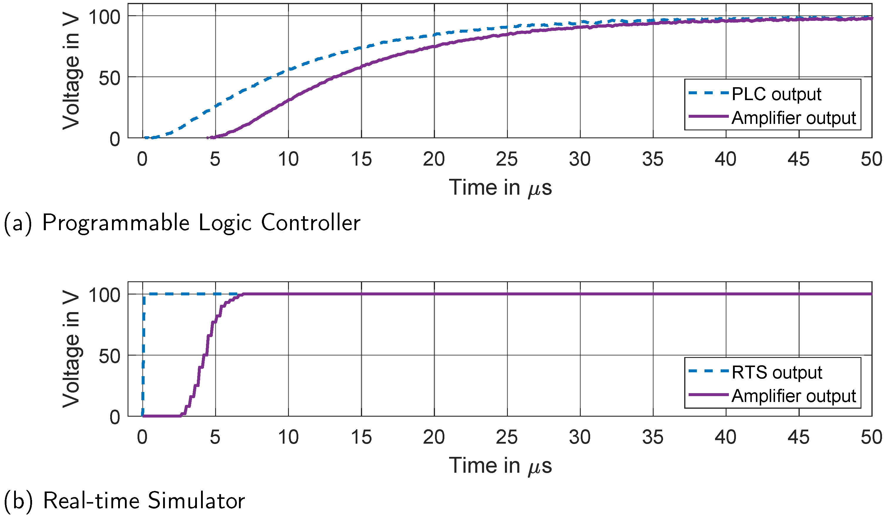
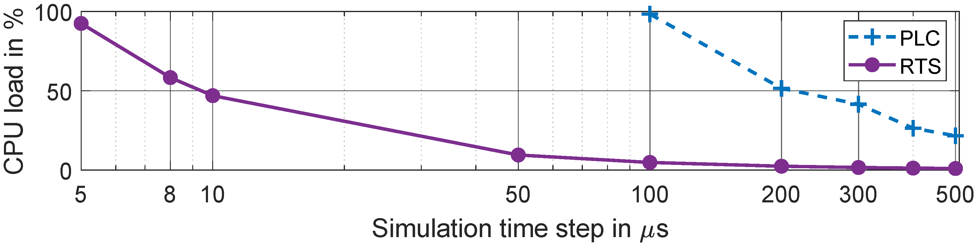
4.1. Comparison of the Bachmann PLC with the OPAL-RT RTS
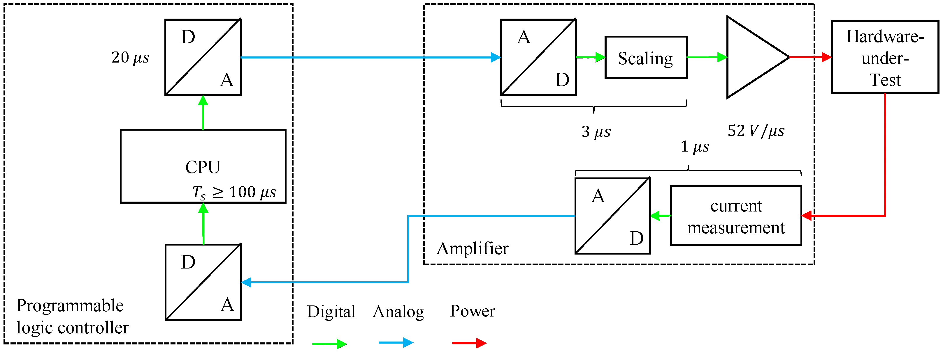
In most PHiL setups, a dedicated RTS is used. They offer high performance to simulate complex models in time steps sufficient for the use in a hardware-connected setup. Depending on the time constant of the simulated as well as the hardware part of the PHiL setup, simulation time steps below 100 μs are needed. In such a case, the setup has to contain an RTS.
If the simulation model is less complex or higher time steps are sufficient for the carried out investigation, less specialized hardware for the simulation might be sufficient. PLCs are normally used as controllers for microgrids or plants [21,22]. They are equipped with a variety of input and output possibilities and execute models in time steps of microseconds. Therefore, they might be used as the simulator in a PHiL setup.
In the following, the OPAL-RT RTS and the Bachmann PLC are compared using the Spitzenberger & Spies amplifier for both simulators. The RTS is connected to the amplifier via its optical connection and the PLC is connected using an analog output module. The setup for the analog connection is shown in Figure 4.
The set point produced by the simulation on the CPU has to be converted into an analog output signal, which is sent to the amplifier. Since the amplifier has an internal digital control, the analog signal has to be converted into a digital signal again. This digital signal is scaled according to the amplification settings and used as the set point for the linear amplifier. The amplifier provides a voltage for the HUT and measures the current. The current measurement is again converted to an analog signal and transmitted to the PLC. In the PLC, the signal is converted back to a digital signal and fed into the simulation. The conversions have to be included in the calculation of the closed-loop delay.
An alternative setup for the connection between the simulator and the amplifier is shown in Figure 5. In this setup, an optical link is used instead of an analog link. In comparison to the analog link, the set points for the amplifier as well as the measurement values for the simulator are transmitted digitally. In this connection setup, no A/D conversions are needed, which shortens the closed-loop time delay.
The optical link is established using the Aurora protocol, which is supported by the OPAL-RT RTS and the Spitzenberger & Spies amplifier [23].
In the following, both PHiL setups are compared regarding the delay between a simulated output value and the actual amplifier output. Additionally, the CPU load for an identical simulation model is compared. Models for execution on both simulators are created using MATLAB/Simulink®, which allows for a comparison of the performance of both simulators with a nearly identical model complexity. The models differ only in simulator-specific requirements regarding the structure and specific modules for the connection to the amplifier.

4.1.1. Output Delay

First, the output delay of the amplifier for both simulators is compared. A simple model simulating a step function from 0 V to 100 V is used. As the HUT, a three-phased resistor with 31 Ω per phase is connected.
The Bachmann PLC uses the external input of the amplifier with a maximum input voltage of 10 V, which matches the maximum output voltage of the PLC. The signal is measured and compared to the output signal of the amplifier. The output is measured using a measurement output connector, which adds a delay of 0.8 μs [24].
The optical interface used by the OPAL-RT RTS cannot be measured directly. The measurements are therefore compared to internal measurements by the manufacturer, which also were recorded using a step from 0 V to 100 V [24].
The results for both simulators are shown in Figure 6. It can be seen that the analog output of the PLC (Figure 6a) needs about 25 μs to rise from 10% to 90%. With a delay of approximately 5 μs, the amplifier output follows the input. One can see that the total delay between the simulated value and the amplifier output is dominated by the rise time of the PLC output.
The output of the RTS is shown in Figure 6b. The digital signal rises instantaneously and the output of the amplifier starts to rise with a delay of 4 μs. It reaches its maximum output value after 8 μs.
Comparing the PHiL setup for both simulators, it becomes clear that the optical connection from the simulator output to the amplifier output is superior in terms of delay. In the case of the PLC, the output delay is mainly produced by the rise time of the analog output of the PLC. Therefore, if highly dynamic processes should be investigated, a high-speed digital connection between the simulator and the amplifier is beneficial. If either the used amplifier or the simulator does not support an optical connection between the devices, an analog output module for the simulator with a low rise time should be used.
If the executed investigations do not include highly dynamic processes, the output delay, i.e., the rise time of the PLC might be tolerable. Especially when simulating alternating voltages or currents, the step between two consecutive set points is much lower than 100 V; therefore, the delay of the PLC output is lower as well.

4.1.2. CPU Load

For the CPU performance test, the model shown in Figure 7 is used. It is a mathematical representation of the ENTSO-E interconnected continental European grid, including frequency control reserve (FCR) and automatic frequency restoration reserve (aFRR).
The grid model consists of a turbine generator model, with a rotating mass on the generator shaft. An accelerating power P a leads to a change in frequency f, neglecting mechanical losses:
d f d t = P a · f 0 2 T G · P n · f
Using the rotational energy present in the interconnected system at nominal frequency f 0 related to the system load P n , the grid time constant T G is calculated as
T G = J · ω 0 2 P n .
The dynamic frequency behavior of the interconnected grid model can thus be represented in a simplified way by a feedback integrator (Figure 7). The integrator represents the storage of the energy of the rotating turbine generator system with the grid time constant T G . The feedback of the frequency deviation Δ f is represented by the self-regulation effect K sr , the FCR P FCR , and the aFRR P aFRR . Quantities marked with an asterisk are related to the grid load P n and the nominal frequency f 0 .
The FCR activation is proportional to Δ f with the gain K FCR and is limited to the amount of FCR P FCR , max held in the interconnected system under consideration. In accordance with the specifications of the transmission system operators, the entire primary control reserve tendered in Germany is activated in the event of a frequency deviation of 0.2 Hz.
K FCR = P FCR , max 0.2 Hz
The physically limited power increase of the power plant units is simplified by a maximum gradient rate P ˙ FCR , max . The power gradient of a thermal power plant unit is subject to certain limits [26] due to limited valve setting speeds for controlling the steam mass flow, the dynamics of the turbine, and the need to avoid critical material stresses due to thermal expansion in the steam generator and turbine. With inverter-coupled generation units, the power change can occur in the millisecond range. The startup behavior of hydropower plants, which provide the majority of the FCR, is in the range of seconds to a few minutes [27]. Since the exact course of the mean power gradient of the FCR providers is not known, the assumption is made that the power gradient is just sufficient to meet the specifications of the reference disturbance case, taking into account the grid time constant T G .
The model is implemented on both simulators and connected to the amplifier. A three-phased resistor with 31 Ω per phase is again used as the HUT. The simple HUT allows a comparison of the performance of both simulators in a closed-loop setup without risking instabilities.
To test the performance, the simulation time step is lowered without changing the model. The mean CPU load for both simulators is measured using internal measurements. As one can see in Figure 8, the CPU load for the PLC starts at about 20% for a time step of 500 μs. At a time step of 200 μs, the CPU load rises to 50%. At these simulation time steps, the CPU load for the OPAL is in the lower single digit range, which is barely above the CPU load in idle mode.
A simulation time step of 200 μs is given by Bachmann as the lowest possible time step. Nevertheless, the model runs at a time step of 100 μs with a CPU load of 98.1%. Trying lower time steps leads to a software error at model compilation.
For the OPAL, a simulation time step of 100 μs leads to a CPU load of 5%. Lowering the time step increases the CPU load peaking at 92% for a time step of 5 μs. For the RTS, lower time steps lead to an increase in overflows, which indicates that not all calculations are finished within one time step. Since a time step of 10 μs is given as a lower limit by OPAL-RT for simulations running on the CPU, this result is expected.
Comparing the CPU loads for both simulators, it can be seen that the performance of the RTS exceeds the PLC. For the same CPU load, the RTS is able to calculate the model about 20 times as fast as the PLC. This shows that a dedicated RTS is needed if either low time steps or a high model complexity is required. The model simulated in this example is fairly simple, i.e., just containing a source, a transformer, and a few lines. Figure 9 shows a Simulink model of a 14-node Cigre middle voltage grid [28]. This model is simulated on the RTS with a time step of 100 μs and an average CPU load of 67%. Simulating such a model on the PLC with an appropriate time step is not possible.
It also proves that a PLC is in general able to be used as a simulator for a PHiL setup. If one wants to use a PLC instead of an RTS because of its lower price or its easier handling, the required time step for the model needs to be considered to produce viable results.
Especially in experiments with alternating current, the frequency of the current or voltage output signal has to be considered. Since a new set point is only generated after a simulation time step is finished, a sinusoidal signal is discretized. In Figure 10a, a 50 Hz sinus signal is shown with four different grades of discretization. In Figure 10a, the sinus is discretized with a time step of 5 μs, which corresponds to the lower limit of possible time steps using the RTS. Using this time step, there is no difference from a perfect sinus signal visible. Figure 10b shows a discretization with a time step of 100 μs, the lower limit of time steps for the PLC. There are still 200 steps within one wavelength of the signal, which is viable for a PHiL setup, especially if the output is smoothed by the rise time of the amplifier.
When increasing the time step to 1 ms, the steps in the signal become visible (Figure 10c). Depending on the rise time of the amplifier, this signal is smoothed, but a discretization of 20 steps per period is the minimum for investigations including alternating currents. For a time step of 5 ms (Figure 10d), there are four steps in one period of the 50 Hz sinus, which is not enough to sufficiently represent the desired wave form. If the model complexity does not allow for a lower simulation time step with the used simulator, one has to explore other ways of controlling the amplifier output.

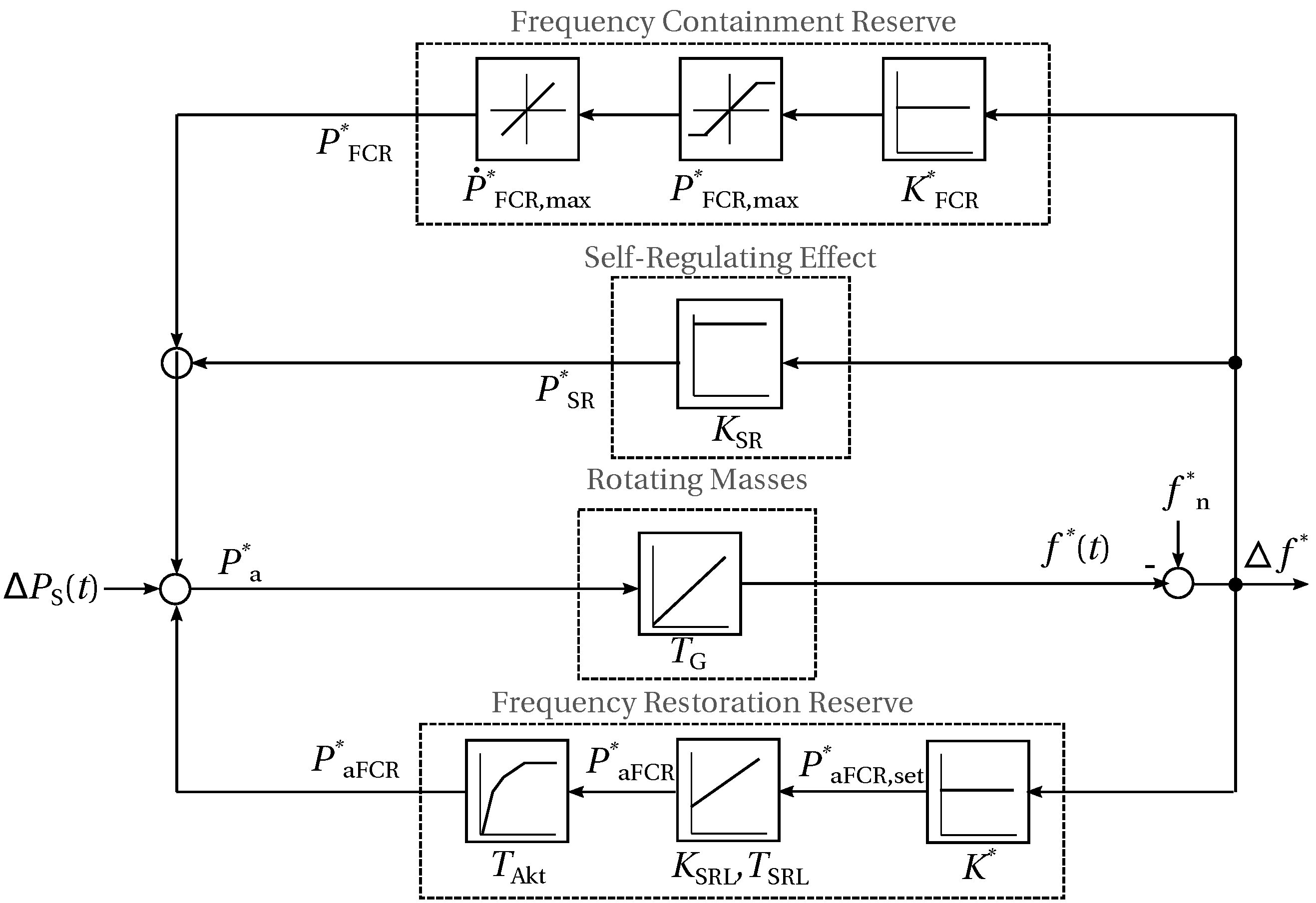
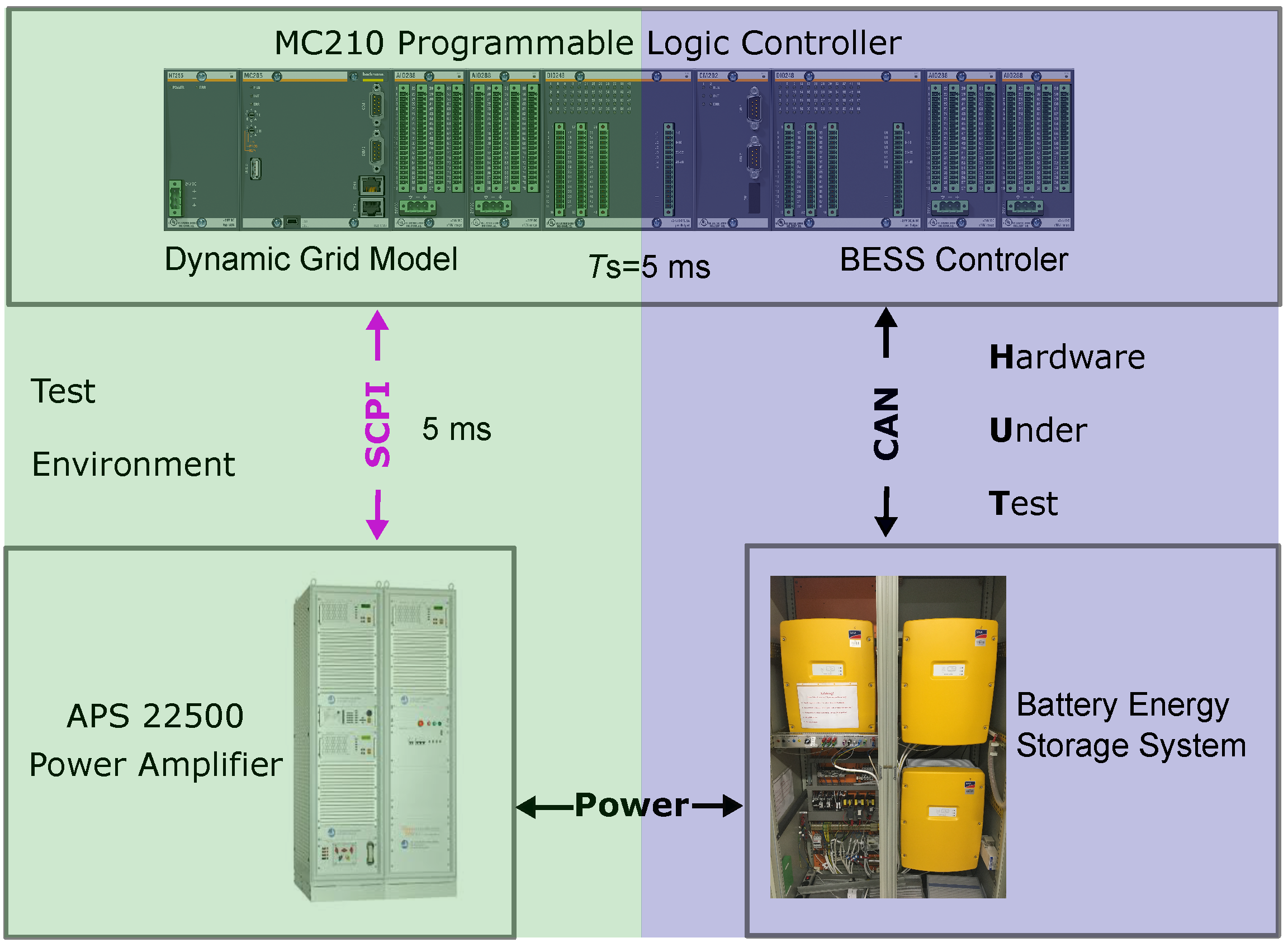
4.2. Impact of Battery Energy Storage Systems for the Provision of FCR in Case of a 3 GW Failure

In order to perform an evaluation of the dynamic behavior of a BESS during the provision of FCR or virtual inertia and to make a statement about the advantages of using BESS for frequency stability in the ENTSO-E power grid with a high share of renewable energies, the reference incident can be used as a scenario.
The reference incident, defined by ENTSOE-E for the continental European interconnected grid, provides a basis for the design of the control reserve. It assumes a sudden outage of two large power plants with a combined capacity of 3 GW during an off-peak time with P n = 150 GW. The outage corresponds to a load jump of 2% of the total load. According to the ENTSO-E guidelines, it shall be ensured that a deviation of the grid frequency of ± 800 mHz and quasistationary ± 200 mHz from the nominal frequency is not exceeded [29].
The PLC is used to control the BESS as well as for real-time simulation of the dynamic grid model (Figure 7). Depending on the implemented control algorithms, the PLC transmit active power set points to the BESS and, depending on the measured active power, frequency set points by SCPI to the power amplifier. Via the SCPI interface of the amplifier, a new frequency value can be set every 5 ms by an SCPI command.
The experimental set up is shown in Figure 11. The HUT is the BESS controller, also implemented in the PLC, and the BESS itself (Figure 11, purple background). The BESS consists of three bidirectional inverters and a lithium-ion phosphate accumulator with a capacity of 20 kWh. The BESS is connected to the three-phase grid build by the power amplifier. The active power is measured by the internal meter of the amplifier and transferred by SCPI to the PLC. The frequency is measured by an external power meter and is also transferred to the PLC.
Since, in this case example, the smallest occurring time constant is in the order of seconds, it is easily achieved with a time step of 5 ms. Disturbing rounding errors can be neglected due to the calculation with 64 bits. The communication between the PLC and the power amplifier takes place via Ethernet with a maximum transmission delay of 5 ms. SCPI protocol is used to send frequency and voltage set points to the internal oscillators of the amplifier. Therefore, unlike the previous case, where the sinus of the voltage was generated in the simulation, in this case, the internal oscillators of the amplifier are used to convert the set points of voltage and frequency into a three-phase sinusoidal signal. This leads to the advantages that the time step of the simulation has no impact on the quality of the sinus voltage and the CPU load can be reduced. Therefore, the time delay of the SCPI communication is negligible given the simulation time step of 5 ms. This case example shows that complex investigations can be implemented without the use of an RTS.

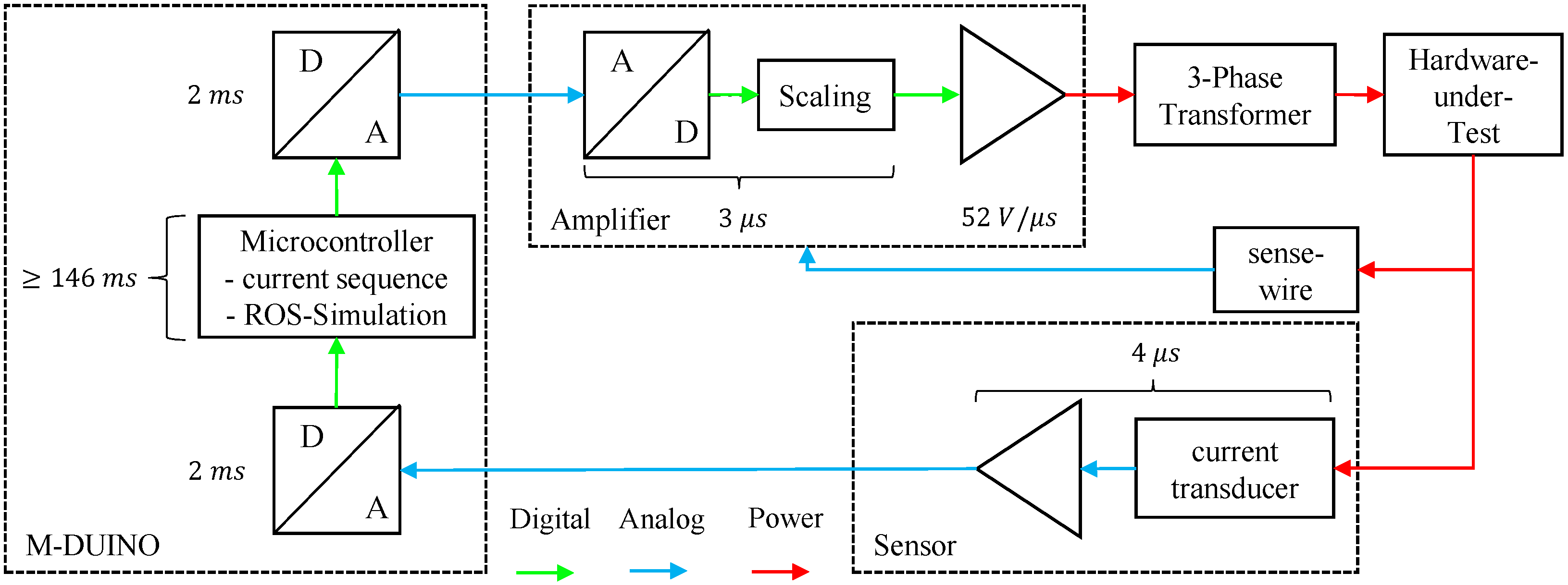
4.3. Closed Loop Control Current Stage

As explained in the case example in Section 4.1, most PHiL setups require a high-performance RTS, but the PHiLsLAB can also be used to test hardware for high current applications with basic simulation hardware. The investigation of current durability of welded or other connections using a current driven measurement setup is presented in this case example. Analogous to the case example in Section 4.2, the internal oscillators of the linear amplifier are used. The used setup and time delays are shown in Figure 12. A basic industrial M-DUINO microcontroller of type M-DUINO 38R+ programmed in C with the Arduino IDE is used for simulating the ROS and controlling the power amplifier. Scaling the power amplifier input is possible, if necessary due to damping and inaccuracies. In the amplifier, the analog input signal is first converted into a digital signal and then triggers an amplitude modulation of the set signal. The current root mean square value, frequency, and phase are preset for this signal; the amplifier is working in current controlled mode and high currents of up to 800 A can be transmitted to the HUT.
This setup can be realized as an open- or closed-loop simulation. For the closed-loop simulation, it is possible to use either the microcontroller and implement, e.g., a PID controller or to use the internal control of the power amplifier.
Using the microcontroller, a current transducer as current sensor is measuring at the HUT and the measured values are being communicated back to the microcontroller via its analog inputs. To use the internal control of the power amplifier to compensate the resistivity of the wires to the HUT that are not part of the HUT, the sense wires need to be connected to the corresponding connection points on the HUT.
The setup can also be realized as open-loop if the mapping is sufficiently exact and the accuracy of the current sequence in the HUT is reasonable. Communication via analog signals supports fast and low-cost implementation on the microcontroller, but it is susceptible to noise. Additional security measures such as temperature limits can be programmed to the microcontroller to stop simulation or start cooling to prevent fire hazard.
Time delays sum up to a total time delay of approximately 148 ms as the M-DUINO time delay is dominating. Thus, the controller is slow due to the M-DUINO, but for current sequences of up to 10 min per step, this is compliant. Additionally, the A/D conversion of the M-DUINO in the feedback loop is adding delay time, but a faster feedback loop can be implemented, when using the sense wires of the amplifier instead of the transducers in connection with measurement cards. Additionally, a faster simulator could minimize the dominating time delay and achieve a faster setting time.

5. Conclusions

PHiL investigations allow an easy and reproducible test setup for hardware used in power and energy systems. This work explains the devices and connections necessary to build a PHiL laboratory and explores different successful applications of PHiL at TU Hamburg PHiLsLab with the aim of recommending different hardware setups adapted to different investigations.
For the implementation of a PHiL laboratory, it is important to consider and match the respective time delays of simulation, amplification, and application. It is shown that the laboratory allows for fast implementation of PHiL setups with either a PLC, a microcontroller, or an RTS as the simulator. Therefore, depending on the necessary performance and time steps, a lower-priced low-end or a more expensive middle- to high-end simulation hardware can be used.
Table 1 shows an overview of the delays produced by the different parts of the PHiL setup. The following recommendations can be derived based on our investigations. For the simulator, first, the simulation time step should be chosen according to the time constant of the ROS. Simulating electromagnetic transients requires a lower time step for higher frequencies, e.g., when harmonics in the power system are investigated. Mathematical models or phasor-based simulations are generally less dynamic and can therefore be simulated at a higher time step. Secondly, the simulator has to be able to calculate the model at that time step. Larger, more complex models have to be simulated on an RTS, whereas smaller models can be simulated on a PLC or even a microcontroller.
The communication protocol as well as the amplifier have to fit the time step of the simulation. Simulating a new set point every 5 μs makes little sense if SCPI is used to transmit the set point just every 200 μs. An M-DUINO microcontroller does not need a high-speed digital connection. In the experiments shown here, the versatile Spitzenberger & Spies amplifier is used. It supports a wide array of communication interfaces and has a low rise time. If a more specialized amplifier is to be used, its communication interfaces and the rise time of its output have to match the intended purpose as well.
The different speeds and time delays of the communication between simulator and amplifier, as well as the feedback, influence the dynamic interaction between the ROS and the HUT and have to be chosen accordingly. The time delays produced by the setup have to be below the dynamics of the investigation to achieve the required precision and avoid instabilities. Depending on the investigated phenomena and their time constants, analog or SCPI communication can be feasible or the faster optical communication might be required. Consequently, if the time constants of the components of the PHiL simulation match the simulator performance, PHiL simulations are a flexible and tool that hardware tests in a safe and reproducible environment.

Author Contributions

Conceptualization, J.I., S.M. and L.W.; methodology, J.I., S.M. and L.W.; software, J.I., S.M. and L.W.; investigation, J.I., S.M. and L.W.; writing—original draft preparation, J.I., S.M. and L.W.; writing—review and editing, T.A.K. and C.B.; visualization, J.I., S.M. and L.W.; supervision, T.A.K. and C.B. All authors have read and agreed to the published version of the manuscript.

Funding

This research was funded as part of an i³ Project, which is an internal research funding program at the Hamburg University of Technology (TUHH).

Institutional Review Board Statement

Not applicable.

Informed Consent Statement

Not applicable.

Data Availability Statement

The data are not publicly available beyond the data presented in the paper since not all involved parties agreed to its publication. For further information regarding the presented data and beyond, please contact the corresponding author.

Acknowledgments

We acknowledge support for the Open Access fees by Hamburg University of Technology (TUHH) in the funding program Open Access Publishing.

Conflicts of Interest

The authors declare no conflict of interest.

Abbreviations

The following abbreviations are used in this manuscript:
BESSBattery Energy Management System
CHiLController Hardware-in-the-Loop
FCRFrequency Containment Reserve
FPGAField Programmable Gate Array
HUTHardware Under Test
PHiLPower Hardware-in-the-Loop
PHiLsLabPower Hardware-in-the-Loop Simulation Laboratory
PLCProgrammable Logic Controller
ROSRest of System
RTSReal-time Simulator
SCPIStandard Commands for Programmable Instruments

References

  1. Ertugrul, N.; Abbott, D. DC is the Future [Point of View]. Proc. IEEE 2020, 108, 615–624. [Google Scholar] [CrossRef]
  2. van Nguyen, H.; Besanger, Y.; Tran, Q.T.; Boudinnet, C.; Nguyen, T.L.; Brandl, R.; Strasser, T.I. Using power-hardware-in-the-loop experiments together with co-simulation for the holistic validation of cyber-physical energy systems. In Proceedings of the 2017 IEEE PES Innovative Smart Grid Technologies Conference Europe (ISGT-Europe), Torino, Italy, 26–29 September 2017; pp. 1–6. [Google Scholar] [CrossRef] [Green Version]
  3. Geisbuesch, J.; Karrari, S.; Kreideweis, P.; de Sousa, B.; Tiago, W.; Noe, M. Set-Up of a Dynamic Multi-Purpose Power-Hardware-in-the-Loop System for New Technologies Integration. In Proceedings of the 2018 IEEE Workshop on Complexity in Engineering (COMPENG), Florence, Italy, 10–12 October 2018; pp. 1–5. [Google Scholar] [CrossRef]
  4. Edrington, C.S.; Steurer, M.; Langston, J.; El-Mezyani, T.; Schoder, K. Role of Power Hardware in the Loop in Modeling and Simulation for Experimentation in Power and Energy Systems. Proc. IEEE 2015, 103, 2401–2409. [Google Scholar] [CrossRef]
  5. Langston, J.; Sloderbeck, M.; Steurer, M.; Dalessandro, D.; Fikse, T. Role of hardware-in-the-loop simulation testing in transitioning new technology to the ship. In Proceedings of the 2013 IEEE Electric Ship Technologies Symposium (ESTS), Arlington, VA, USA, 22–24 April 2013; pp. 514–519. [Google Scholar] [CrossRef]
  6. Yamane, A.; Rangineed, T.; Gregoire, L.A.; Ali, S.Q.; Paquin, J.N.; Belanger, J. Multi-FPGA Solution for Large Power Systems and Microgrids Real Time Simulation. In Proceedings of the 2019 IEEE Conference on Power Electronics and Renewable Energy (CPERE), Aswan, Egypt, 23–25 October 2019; pp. 367–370. [Google Scholar] [CrossRef]
  7. Saad, H.; Ould-Bachir, T.; Mahseredjian, J.; Dufour, C.; Dennetiere, S.; Nguefeu, S. Real-Time Simulation of MMCs Using CPU and FPGA. IEEE Trans. Power Electron. 2015, 30, 259–267. [Google Scholar] [CrossRef]
  8. Bachmann Electronic GmbH. Bachmann System Overview; Datasheet: Feldkirch, Germany, 2019; Available online: https://www.bachmann.info/en/issuu-pages/systemoverview-2020-english/ (accessed on 27 May 2021).
  9. Zhang, P. Industrial Control Technology: A Handbook for Engineers and Researchers; William Andrew: Norwich, NY, USA, 2008. [Google Scholar]
  10. Lehfuss, F.; Lauss, G.; Kotsampopoulos, P.; Hatziargyriou, N.; Crolla, P.; Roscoe, A. Comparison of multiple power amplification types for power Hardware-in-the-Loop applications. In Proceedings of the 2012 Complexity in Engineering (COMPENG), Aachen, Germany, 11–13 June 2012; pp. 1–6. [Google Scholar] [CrossRef] [Green Version]
  11. Ren, W.; Steurer, M.; Baldwin, T.L. An Effective Method for Evaluating the Accuracy of Power Hardware-in-the-Loop Simulations. IEEE Trans. Ind. Appl. 2009, 45, 1484–1490. [Google Scholar] [CrossRef]
  12. Viehweider, A.; Lauss, G.; Felix, L. Stabilization of Power Hardware-in-the-Loop simulations of electric energy systems. Simul. Model. Pract. Theory 2011, 19, 1699–1708. [Google Scholar] [CrossRef]
  13. Ren, W.; Steurer, M.; Baldwin, T.L. (Eds.) Improve the Stability and the Accuracy of Power Hardware-in-the-Loop Simulation by Selecting Appropriate Interface Algorithms. IEEE Trans. Ind. Appl. 2008. [Google Scholar] [CrossRef]
  14. de Jong, E.; de Graff, R.; Vassen, P.; Crolla, P.; Roscoe, A.; Lefuss, F.; Lauss, G.; Kotsampopoulos, P.; Gafaro, F. European White Book on Real-Time Powerhardware-in-the-Loop Testing International White Book on DER Protection: Review and Testing Procedures; DERlab Report; DERlab e.V.—European Distributed Energy Resources Laboratories: Hessen, Germany, 2012; ISBN 978-3-943517-01-9. [Google Scholar]
  15. Roscoe, A.J.; Mackay, A.; Burt, G.M.; McDonald, J.R. Architecture of a Network-in-the-Loop Environment for Characterizing AC Power-System Behavior. IEEE Trans. Ind. Electron. 2010, 57, 1245–1253. [Google Scholar] [CrossRef] [Green Version]
  16. Montoya, J.; Brandl, R.; Vishwanath, K.; Johnson, J.; Darbali-Zamora, R.; Summers, A.; Hashimoto, J.; Kikusato, H.; Ustun, T.S.; Ninad, N.; et al. Advanced Laboratory Testing Methods Using Real-Time Simulation and Hardware-in-the-Loop Techniques: A Survey of Smart Grid International Research Facility Network Activities. Energies 2020, 13, 3267. [Google Scholar] [CrossRef]
  17. Spitzenberger & Spies. APS Series of 4-Quadrant Amplifiers, Datasheet. 2021. Available online: https://spitzenberger.de/weblink/1107 (accessed on 26 February 2021).
  18. Bachmann Electronic GmbH. Manual MC210. Available online: https://www.bachmann.info/fileadmin/media/Produkte/Steuerungssystem/Produktblaetter/MC200-Serie_de.pdf (accessed on 22 January 2021).
  19. OPAL-RT Technologies, Inc. OP5600V2—Hardware Products Documentation—Wiki OPAL-RT. Available online: https://wiki.opal-rt.com/display/HDGD/OP5600V2 (accessed on 21 January 2021).
  20. Mathworks. MATLAB&Simulink. 2019. Available online: https://de.mathworks.com/help/releases/R2019b/pdf_doc/simulink/slref.pdf (accessed on 26 February 2021).
  21. Kumar, Y.P.; Bhimasingu, R. Alternative hardware-in-the-loop (HIL) setups for real-time simulation and testing of microgrids. In Proceedings of the 2016 IEEE 1st International Conference on Power Electronics, Intelligent Control and Energy Systems (ICPEICES), Delhi, India, 4–6 July 2016; pp. 1–6. [Google Scholar] [CrossRef]
  22. Reddy, Y.J.; Ramsesh, A.; Raju, K.P.; Kumar, Y. A novel approach for modeling and simulation of hybrid power systems using PLCs and SCADA for hardware in the loop test. In Proceedings of the International Conference on Sustainable Energy and Intelligent Systems (SEISCON 2011), Chennai, India, 20–22 July 2011; pp. 545–553. [Google Scholar] [CrossRef]
  23. Xilinx. Inc. Aurora Protocol Specification. Available online: https://www.xilinx.com/support/documentation/ip_documentation/aurora_8b10b_protocol_spec_sp002.pdf (accessed on 1 March 2021).
  24. Spitzenberger & Spies. Advantages of linear amplifiers in Power Hardware In the Loop applications, Presentation. 2021. Available online: https://spitzenberger.de/weblink/1135 (accessed on 26 February 2021).
  25. Wilkening, L.; Ackermann, G.; Becker, C. Netzorientierter Betrieb von Batteriespeichersystemen in Verteilnetzen. Ph.D. Thesis, Technische Universität Hamburg, Hamburg, Germany, 2021. [Google Scholar]
  26. Handschin, E.; Petroianu, A. Energy Management Systems: Operation and Control of Electric Energy Transmission Systems; Electric Energy Systems and Engineering Series; Springer: Berlin/Heidelberg, Germany; New York, NY, USA; London, UK; Paris, France; Tokyo, Japan; Hong Kong, China; Barcelona, Spain; Budapest, Hungary, 1991. [Google Scholar]
  27. Sayigh, A.; Lejeune, A.G.H. Comprehensive Renewable Energy (Hydro Power/vol. ed. André G.H. Lejeune); Elsevier: Amsterdam, The Netherlands, 2012; Volume 6. [Google Scholar]
  28. Barsali, S.; Tf, C. Benchmark Systems for Network Integration of Renewable and Distributed Energy Resources. 2014. Available online: http://e-cigre.org/publication/ELT_273_8-benchmark-systems-for-network-integration-of-renewable-and-distributed-energy-resources (accessed on 27 May 2021).
  29. The European Commission. Commission Regulation (EU) 2017/1485 Establishing a Guideline on Electricity Transmission System Operation. 25 August 2017, pp. 1–120, In Force: This Act Has Been Changed. Current Consolidated Version: 15 March 2021. Available online: http://data.europa.eu/eli/reg/2017/1485/oj (accessed on 27 May 2021).
Figure 1. General power hardware-in-the-loop setup.
Energies 14 03154 g001
Figure 2. PHiLsLAB at TU Hamburg.
Energies 14 03154 g002
Figure 3. Possible PHiL setups in PHiLsLab.
Energies 14 03154 g003
Figure 4. PHiL with analog communication between the PLC and the amplifier.
Energies 14 03154 g004
Figure 5. PHiL with digital communication between the RTS and the amplifier.
Energies 14 03154 g005
Figure 6. Simulator output, compared to the amplifier output for the Bachmann PLC (a) and the OPAL-RT RTS (b). Values of (b) are according to [24].
Energies 14 03154 g006
Figure 7. Block diagram of the dynamic ENTSO-E grid model [25].
Energies 14 03154 g007
Figure 8. CPU load for the Bachmann MC210 and the OPAL OP5600 for different simulation time steps.
Energies 14 03154 g008
Figure 9. Simulink model of a threephased middle voltage grid.
Energies 14 03154 g009
Figure 10. Discretised sinusoidal signal with a time step of 5 μs (a), 100 μs (b), 1 ms (c), and 5 ms (d).
Energies 14 03154 g010
Figure 11. PHiL with digital communication between PLC and amplifier (Ethernet/SCPI) and between PLC and BESS (CAN BUS).
Energies 14 03154 g011
Figure 12. Measurement setup closed-loop control current stage.
Energies 14 03154 g012
Table 1. Time delays.
DeviceMinimum Time Delay
Simulator time step:
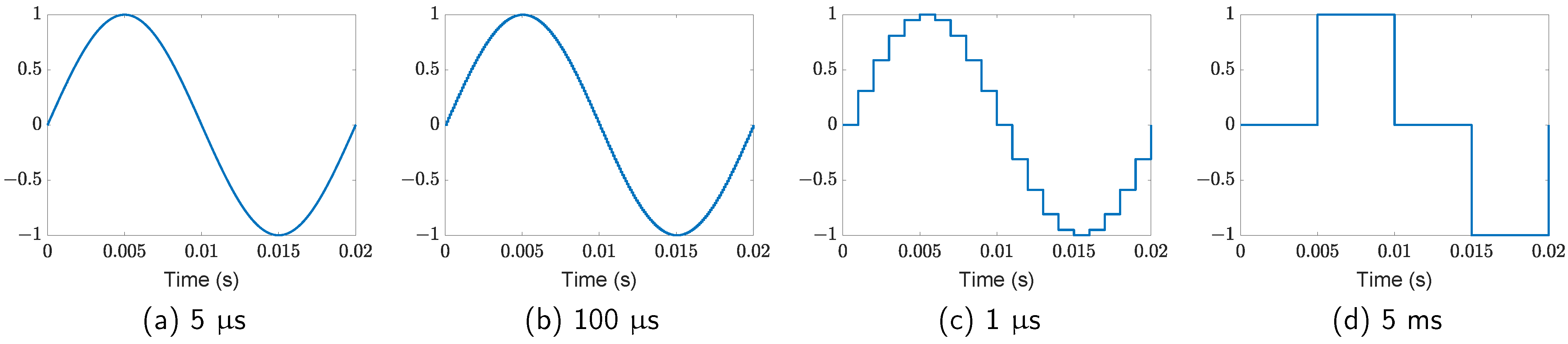
OPAL-RTS5 μs
Bachmann PLC100 μs
M-DUINO μC146 ms
Communication delay including conversions:
OPAL-RTS Aurora1 μs
Bachmann PLC analog20 μs
Bachmann PLC SCPI122 μs
M-DUINO analog μC2 ms
linear amplifier read-in:
Spitzenberger & Spies APS digital1 μs
Spitzenberger & Spies APS analog3 μs
Spitzenberger & Spies APS SCPI5 ms
Publisher’s Note: MDPI stays neutral with regard to jurisdictional claims in published maps and institutional affiliations.

