Article

MRAS-Based Switching Linear Feedback Strategy for Sensorless Speed Control of Induction Motor Drives

by
Mohamed Amine Fnaiech
1,*,
Jaroslaw Guzinski
2,
Mohamed Trabelsi
3,
Abdellah Kouzou
4,5,
Mohamed Benbouzid
6,7 and
Krzysztof Luksza
2
1
Department of Electrical and Electronics Engineering, College of Engineering, University of Bahrain, Isa Town, Zallaq 32038, Bahrain
2
Department of Electric Drives and Energy Conversion, Faculty of Electrical and Control Engineering, Gdańsk University of Technology, Narutowicza 11/12, 80-233 Gdańsk, Poland
3
Department of Electronic and Communications Engineering, Kuwait College of Science and Technology, Doha District, Block 4, Doha 27235, Kuwait
4
Applied Automation and Industrial Diagnosis Laboratory (LAADI), Faculty of Science and Technology, Djelfa University, Djelfa 17000, Algeria
5
Electrical and Electronics Engineering Department, Nisantasi University, Istanbul 34398, Turkey
6
Institut de Recherche Dupuy de Lome, University of Brest, 29238 Brest, France
7
Logistics Engineering College, Shanghai Maritime University, Shanghai 201306, China
*
Author to whom correspondence should be addressed.
Energies 2021, 14(11), 3083; https://doi.org/10.3390/en14113083
Submission received: 17 April 2021 / Revised: 16 May 2021 / Accepted: 21 May 2021 / Published: 26 May 2021
(This article belongs to the Special Issue Applications of Modern Methods to Control of Electric Drives)

Abstract

:
This paper presents a newly designed switching linear feedback structure of sliding mode control (SLF-SMC) plugged with an model reference adaptive system (MRAS) based sensorless field-oriented control (SFOC) for induction motor (IM). Indeed, the performance of the MRAS depends mainly on the operating point and the parametric variation of the IM. Hence, the sliding mode control (SMC) could be considered a good control alternative due to its easy implementation and robustness. Simulation and experimentation results are presented to show the superiority of the proposed SLF-SMC technique in comparison with the classical PI controller under different speed ranges and inertia conditions.

1. Introduction

The increasing use of controlled speed sensorless induction motors (IM) in the industry is due to the advance in digital signal processing (DSP) techniques and high capabilities of new microprocessor technologies [1]. Indeed, the suppression of the mechanical speed sensor from the rotor shaft leads to less bulky drive systems with higher reliability and robustness. In this context, the model reference adaptive system (MRAS) estimator has shown the best performance and has become a privileged solution for sensorless field-oriented control (SFOC) of IM due to its simple design (based on the IM electrical model) and high reliability [2].
The design of the MRAS estimator is based on two sets of equations, where only one set includes the variable to be estimated. The set of equations that does not include the estimated variable is called the reference model, while the other one is called the adaptive model. The error between the estimated quantities obtained by the two models is used to drive a suitable adaptation mechanism, which generates the estimated variable for the adjustable (adaptive) model. The use of the differential equations of the IM rotor flux for both reference and adaptive models was first introduced in [2,3,4]. This structure is well discussed in the literature, where the determined transfer function allows for the modelling of the MRAS dynamics (interesting feature for transient analysis) [5].
The MRAS estimator is defined through its adaptation mechanism, where the new mechanical dynamics that is adjusted by the outer control-loop is dedicated to the rotor speed. Therefore, the substitution of the measured speed by the estimated one in the control-loop causes some performance variation of the overall closed-loop control system, and this variation becomes more important when the mechanical system undergoes some parametric variations such as inertia change. However, many industrial processes using controlled IM do not allow for any change of their dynamics when replacing the field-oriented control (FOC) by sensorless field-oriented control (SFOC). In order to overcome this issue, it is required to adjust the parameters of the adaptation mechanism in order to maintain the original performance. In addition, the most widely used adaptation mechanism is the classical proportional-integral controller (PI), where the tuning of two parameters at the time for different operating condition is complex [2,4,5].
The performance of the MRAS at low speed has been widely discussed in the literature. Indeed, most of the works have focussed on the idea of replacing the PI controller by another more advanced controller in order to improve the performance at low speed, which is influenced by some parametric variations and the nonlinearity of the converter. Intelligent algorithm such as linear neural network and fuzzy logic controllers have been developed respectively in [4,6], while model predictive control has been proposed in [7]. All of these techniques show better performance compared to the PI controller for steady-state at low speed operation modes. However, the transient analysis of the MRAS has not been addressed in previous research because the dynamics of the MRAS cannot vary and match the real dynamics of the mechanical part. The ideal solution is to develop a simple and robust algorithm for the MRAS adaptation mechanism, such as sliding mode control (SMC), which can adapt and impose a dynamic similar to the real dynamics of the machine [8].
The SMC has found a wide range of applications in electrical engineering due to its low computational burden, easy implementation, and non-sensitivity to the parameters variation [8,9,10]. The application of the SMC on MRAS based SFOC for IM was presented in many previous works [4,5,11,12,13,14]. In [4,5,12,13,14], the switching gain and equivalent signal structures of SMC were developed for two different designs of MRAS: the first one is based on rotor flux, while the second one is based on stator current. The results obtained for the switching gain structure are characterized by a high chattering phenomenon [5,14]. Moreover, those obtained with the equivalent command show a robustness that is very dependent on the discontinuous control signal [4,12,13]. To avoid dependency and chattering problems, MRAS-based second-order sliding mode control was proposed in [11]. However the Lyapunov stability condition of this structure is hardly achieved through the tuning of three parameters [15,16,17]. The switching linear feedback structure is considered as a good compromise between all structures of SMC. Indeed, the design is based on the model of system, where the switching element and the generated control signal depend on the error between desired and measured values. Therefore, the SLF-SMC is characterized by a good robustness performance at low chattering phenomena.
According to the above-discussed literature review shortcomings and highlights, the contribution of this paper is the application of the SLF-SMC for MRAS-based SFOC for IM. The proposed SLF-SMC is applied to the classical rotor flux-based MRAS [5]. The performance of the SLF-SMC is evaluated and compared with that offered by a conventional PI controller under different speed range and inertia conditions.
The remaining of this paper is organized as follows. In Section 2, preliminaries about the MRAS based on differential equation of the IM rotor flux and the design methodology of the SLF-SMC are presented. The Section 3 presents the comparative simulation results between SLF-SMC and PI controller. The results of experimental validation are presented in Section 4. Concluding remarks and possible future research directions are outlined in Section 5. For future applications and results reproducibility, the proposed MRAS-SMC algorithm codes are made available as Supplementary Materials.

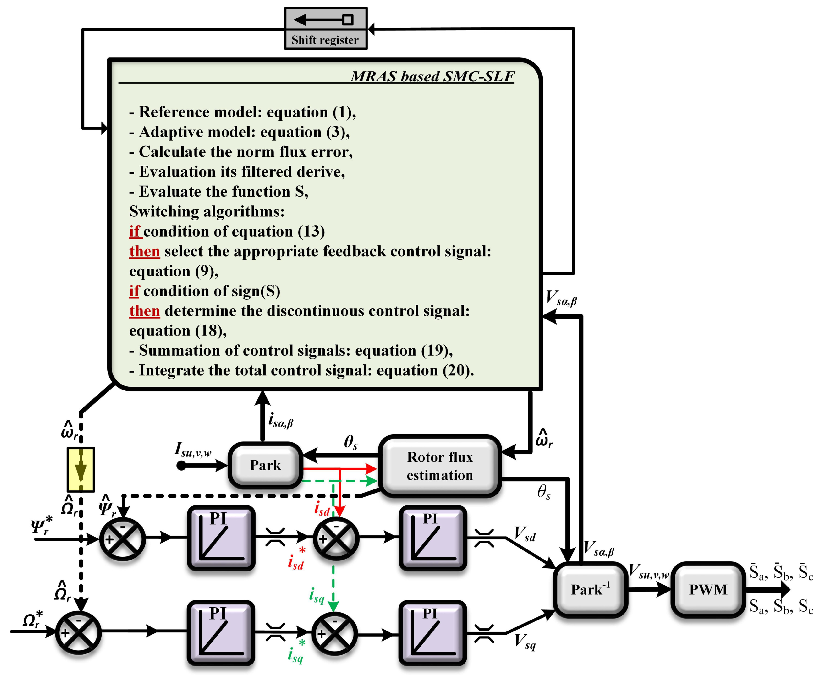
2. SLF-SMC for MRAS Estimator

The application of FOC for IM has been widely discussed in the literature [1,18]. Therefore, theoretical background and analysis in this paper focus on the application of the SLF-SMC for an MRAS estimator.

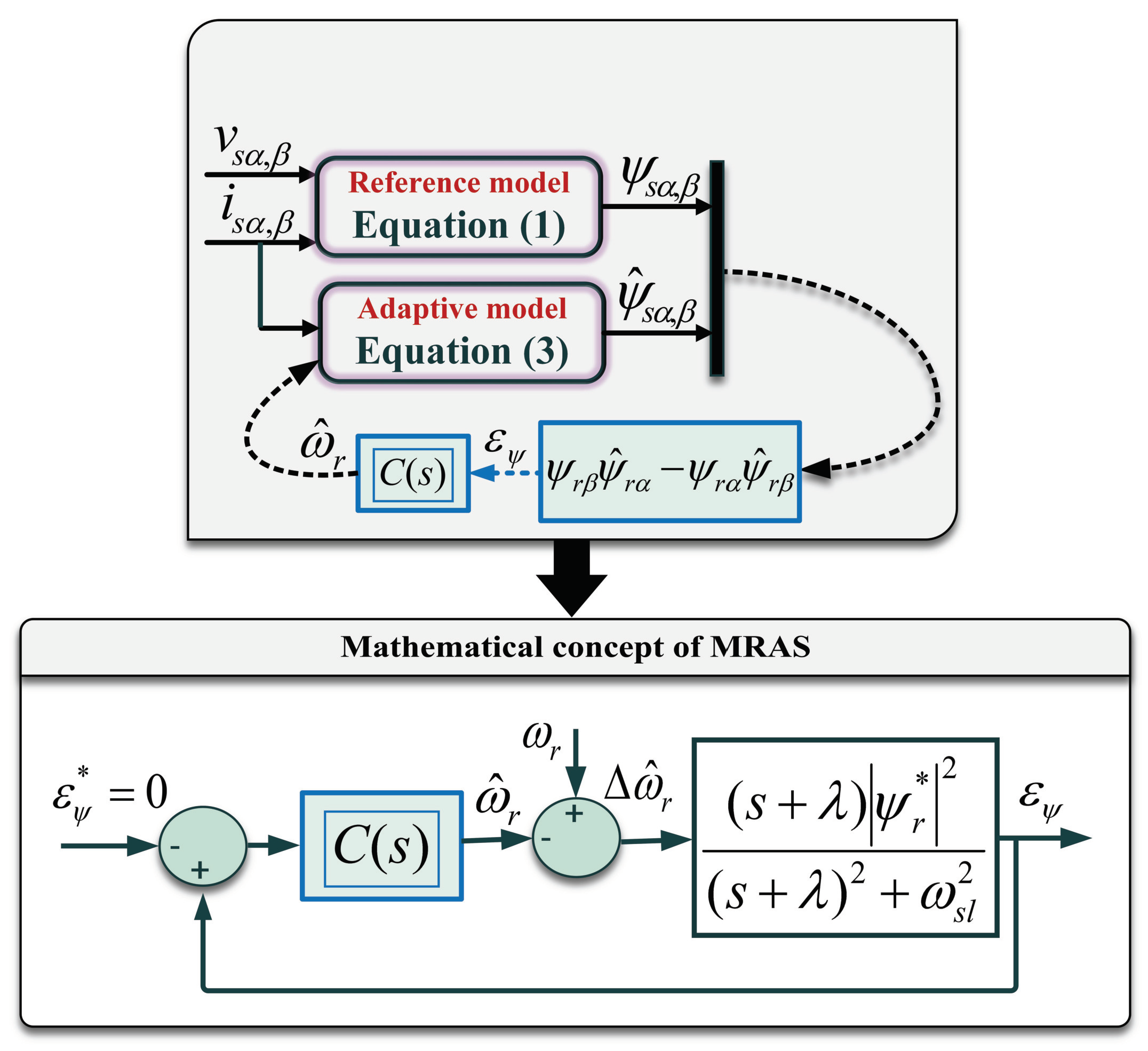
2.1. Preliminaries on MRAS Estimator

The MRAS estimator applied to the IM is based on two sets of differential equations, which allow for the calculation of the rotor flux, where only one of them must includes the variable to be estimated, which is the rotor speed ( ω r ) in this study. In fact, the system that does not include the estimated rotor speed is called a reference Model (1), while the other one is called the adaptive Model (2). The error between the output quantities obtained from two models is used to develop a suitable adaptation mechanism, which generates the estimated rotor speed ω ^ r , for the adjustable model [2,19,20,21].
ψ r α , β = L r L m ( v s α , β R s i s α , β ) s L s σ i s α , β
ψ r α = 1 s λ ψ r α ω r ψ r β + λ L m i s α , ψ r β = 1 s λ ψ r β + ω r ψ r α + λ L m i s β .
Figure 1 shows the design and mathematical theory of the MRAS estimator applied for an IM. To explain the mathematical theory of the MRAS estimator, the estimated rotor speed should be considered first in the adaptive model. Hence, Equation (2) can be rewritten as follows:
ψ ^ r α = 1 s λ ψ ^ r α ω ^ r ψ ^ r β + λ L m i s α , ψ ^ r β = 1 s λ ψ ^ r β + ω ^ r ψ ^ r α + λ L m i s β .
The performance and dynamics of the MRAS were discussed in [2,5]. It was also proven that the transfer function given by Equation (4) links the norm of the flux error to the speed error. It can be expressed as follows:
ε ψ Δ ω ^ r = ( s + λ ) | ψ r * | 2 ( s + λ ) 2 + ω s l 2
where ε ψ = ψ r β ψ ^ r α ψ ^ r β ψ r α and Δ ω ^ r = ω r ω ^ r .
The static gain of the transfer function presented in Equation (4) is approximately equal to 1. Taking into account Popov hyperstability criteria, which implies that, if the norm of the flux error reaches zero ( ε ψ 0 ), then the speed error reaches zero ( Δ ω ^ r 0 ) and consequently ω ^ r reaches ω r [22].
For unknown signal ω r , the goal of the closed-loop control system is to control the norm of the flux error ε ψ to follow its desired zero value ε ψ * . The controller used in the closed-loop generates the desired ω ^ r , which confirms that Δ ω ^ r = 0 . Thus, the estimated rotor speed is calculated by the following:
ω ^ r = C ( s ) ε ψ
where C ( s ) is the controller used for controlling the norm of flux error. It is designed based on the following transfer function that is deduced from Equation (4):
ε ψ ω ^ r = ( s + λ ) | ψ r * | 2 ( s + λ ) 2 + ω s l 2
The research presented in [5,23,24] used the assumption of ω s l = 0 (which is not an accurate assumption) to tune the PI controller. Indeed, this assumption leads to the reduction of the order of the transfer function in Equation (6) (becoming a first order system) so the PI controller parameters are tuned by poles placement.
In this research, an SLF-SMC strategy is proposed for the MRAS estimator, where the design methodology is detailed in the following subsection.

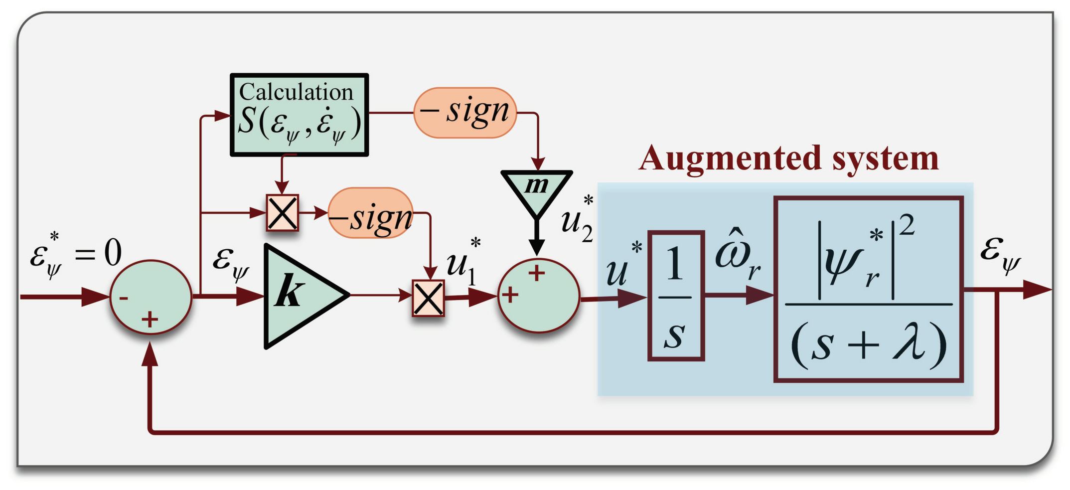
2.2. Design of the SLF-SMC for the MRAS

The mathematical background of the MRAS presented in the previous section leads to a transfer function relating the norm of the flux error to the rotor speed error. This transfer function includes the slip speed ω s l , and therefore, it presents a time-varying system [19,25]. When neglecting ω s l , this transfer function become a first-order transfer function as follows:
ε ψ ω ^ r = | ψ r * | 2 ( s + λ )
This subsection focuses mainly on of the application of the SLF-SMC for the MRAS estimator using the previous Equation (7). It is worth noting that the SLF-SMC can be applied only for second- and higher-order systems. Therefore, the application of this structure to first-order systems requires the addition of integral action in series with the system, as shown in Figure 2.
The augmented system is described by the following second-order transfer function:
ε ψ u * = | ψ r * | 2 ( s 2 + λ s )
with an input control, u * , which is the sum of two terms u 1 * and u 2 * . The value of u 1 * is related to the feedback loop, and u 2 * is a discontinuous signal is added to remove the steady-state error:
u 1 * = k ε ψ f o r F k ε ψ f o r F +
where the negative and positive feedbacks are F and F + . respectively. The constant k must be chosen in such a way as (1) to avoid the permanent saturation of the control signal during the totality of the transient mode and (2) to obtain real and complex poles implying trajectories in phase plane that converge towards the switching surface.
The negative and positive feedbacks lead, respectively, to the following closed-loop transfer functions:
ε ψ ( s ) ε ψ * ( s ) = k | ψ r * | 2 s 2 + λ s + k | ψ r * | 2 f o r F ε ψ ( s ) ε ψ * ( s ) = k | ψ r * | 2 s 2 + λ s k | ψ r * | 2 . f o r F +
In case of negative feedback, the phase plane trajectory has a spiral form where the equilibrium point shows a stable focus. The closed-loop poles ( s 1 n , s 2 n ) are complex with negative real parts as given below:
s 1 n / s 2 n = λ ± j λ 2 + 4 k | ψ r * | 2 2 .
When a positive feedback is applied, the phase plane trajectory consists of a set of hyperbolas with two asymptotes D 1 and D 2 (the equilibrium point presents a saddle), where the slopes are computed by the poles given in Equation (12).
s 1 p / s 2 p = λ ± λ 2 + 4 k | ψ r * | 2 2 .
For a second-order system, a first-order switching surface must be considered as a desired trajectory in the phase plane:
S ( ε ψ , ε ˙ ψ ) = C ε ψ + ε ˙ ψ = 0
where ε ˙ ψ = [ ψ ˙ r β ψ ^ r α + ψ r β ψ ^ ˙ r α ] [ ψ ^ ˙ r β ψ r α + ψ ^ r β ψ ˙ r α ] is calculated using the reference and adaptive models. The design of the SLF-SMC is based on the attractiveness of the switching surface that can be achieved by using the theory of Lyapunov stability for the selected switching surface [26,27,28]. Consider the following Lyapunov function:
V ( ε ψ , ε ˙ ψ ) = S 2 = ( C ε ψ + ε ˙ ψ ) 2
It is obvious that it presents a definite positive function. Its derivative is as follows:
V ˙ = 2 S ˙ S
The stability of Lyapunov imposes that V ˙ must be negative ( V ˙ < 0 ), which means that the following condition has to be satisfied:
S ˙ S < 0
Based on the closed-loop transfer functions presented in Equation (10), if it is assumed that the trajectory in the phase plane is near the switching surface and the closed-loop control system is initially considered with a negative feedback, the stability condition of Lyapunov function given in Equation (16) can be written for the negative and positive feedbacks as follows:
S ( ε ψ , ε ˙ ψ ) ε ψ > 0 t h e n F S ( ε ψ , ε ˙ ψ ) ε ψ < 0 t h e n F +
Considering the result of Lyapunov stability condition mentioned in Equation (16), in the case of parametric disturbance and for a trajectory very close to the switching surface, implies the addition of the discontinuous control signal u 2 * :
u 2 * = m s i g n [ S ( ε ψ , ε ˙ ψ ) ]
where | m | is higher than all magnitudes of the considered parametric disturbances. From all algorithm design steps, the following control signal u * is deducted:
u * = k ε ψ s i g n [ S ( ε ψ , ε ˙ ψ ) ε ψ ] m s i g n [ S ( ε ψ , ε ˙ ψ ) ]
and ω ^ r is deduced as follows:
ω ^ r = k ε ψ s i g n [ S ( ε ψ , ε ˙ ψ ) ε ψ ] m s i g n [ S ( ε ψ , ε ˙ ψ ) ] s
The trajectory in the phase plan is always attracted by the switching line if the slope of the switching surface is selected to be lower than the slopes of s 1 p
C < λ + λ 2 + 4 k | ψ r * | 2 2 .
In fact, by choosing the slope of the sliding surface smaller than that of the asymptote D 1 (slope s 1 p ), this implies that the directions of both spiral and hyperbolas are oriented towards the chosen switching line.

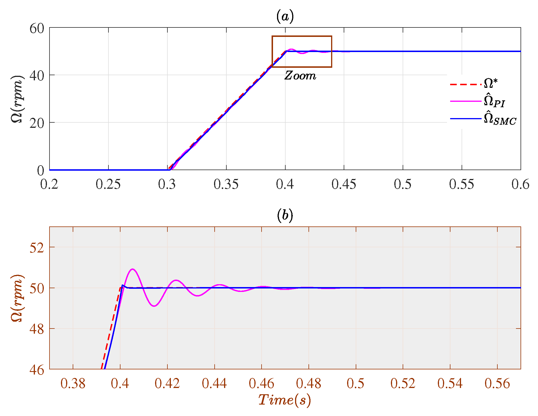
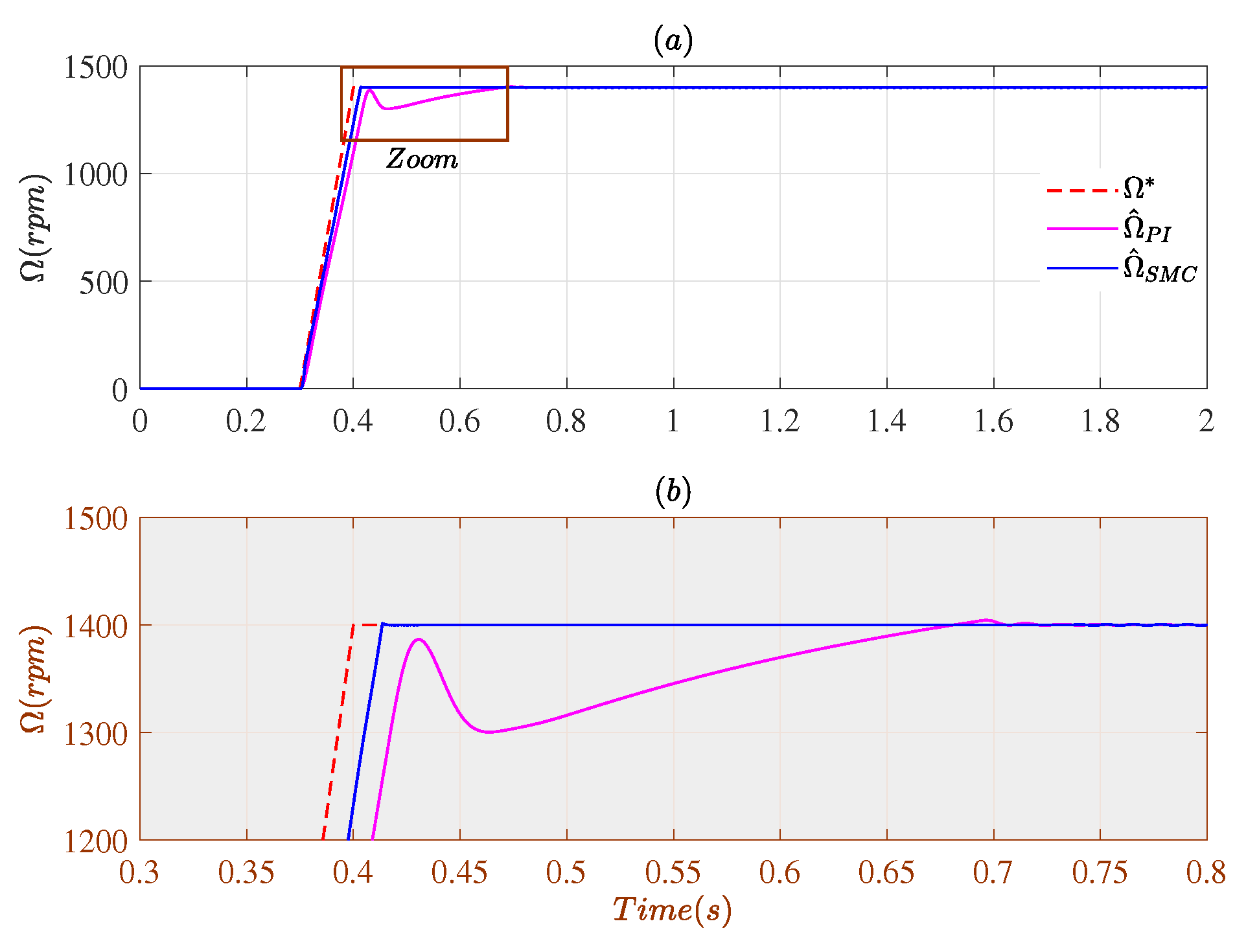
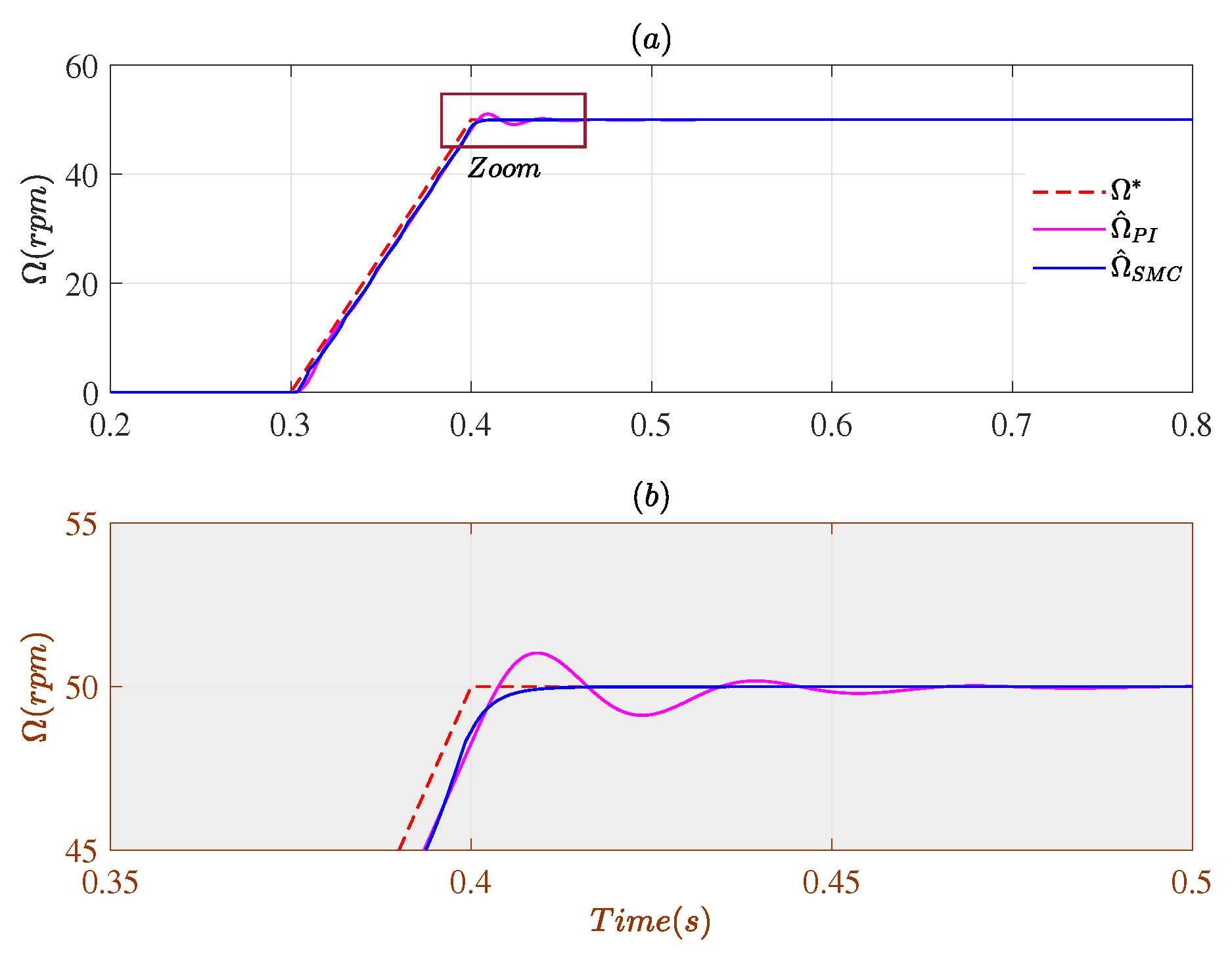
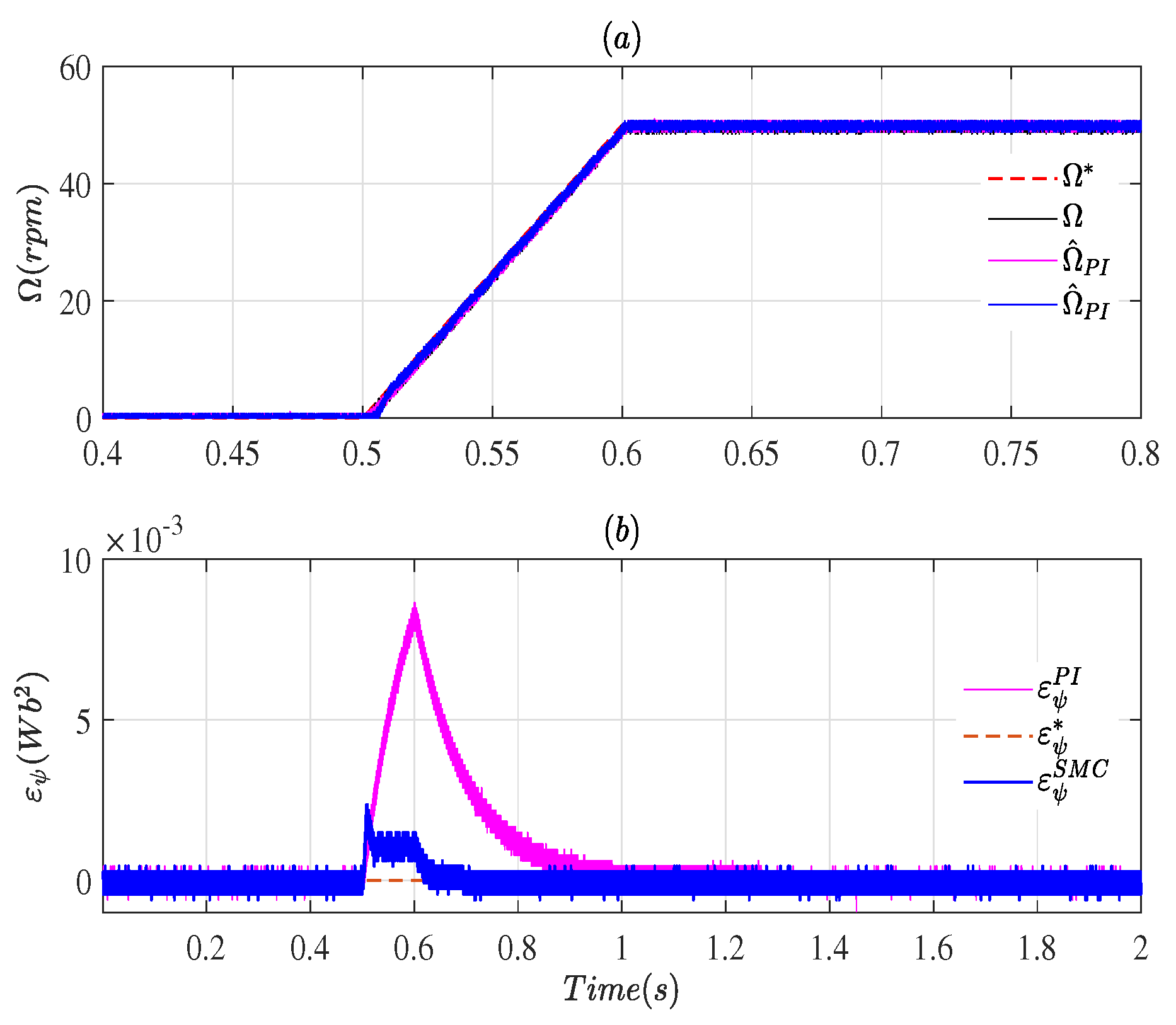
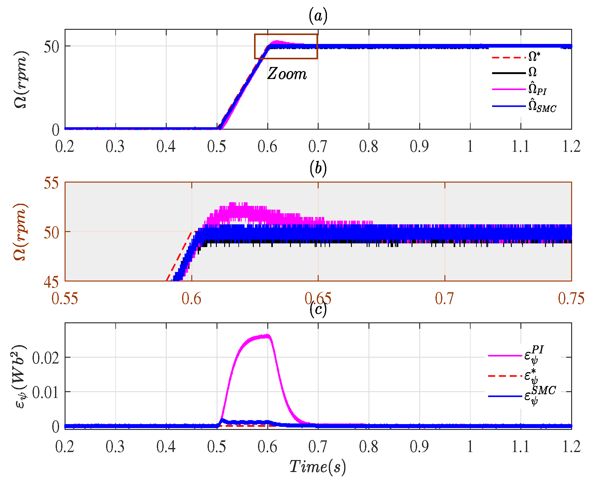
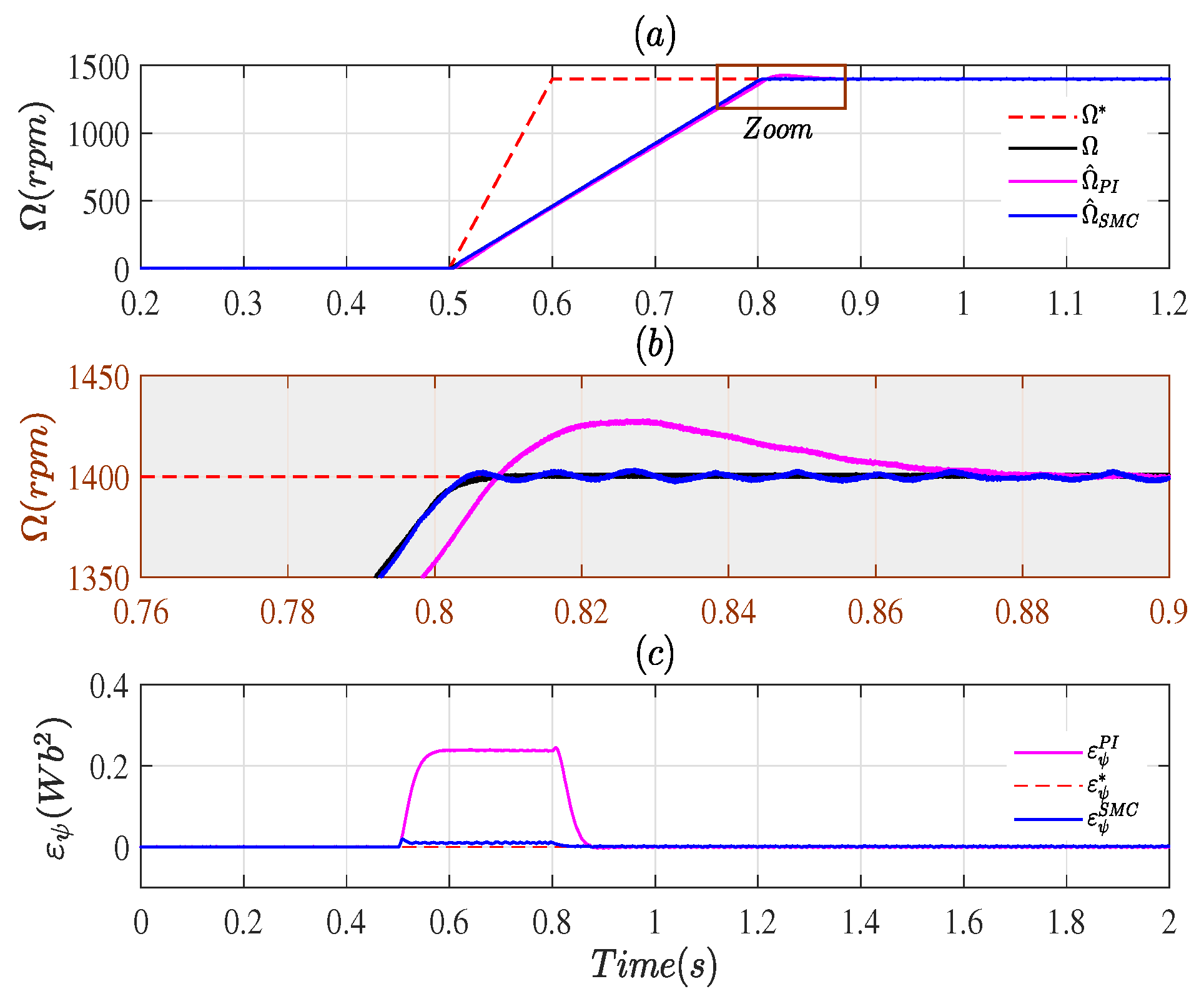
3. Simulation Results

The simulation results were performed in order to compare the performance of the MRAS-based SLF-SMC and PI controller (named MRAS-SMC and MRAS-PI, respectively) under different operation conditions. The simulated system is composed by an IM, a FOC, and an MRAS estimator. All of the parameters of the IM are presented in Table 1. The parameters of SLF-SMC and PI controller are computed to obtain an estimated speed with the same dynamics as the one measured under normal inertia conditions of the IM. Indeed, this step is mandatory to ensure an objective performance comparison in case of SFOC using estimated speeds given by the MRAS-SMC and the MRAS-PI. Based on the application of the compensation pole placement method on the transfer function defined in Equation (20)), the parameters of the PI controller have been calculated ( K p = 10 2 , K i = 4 × 10 3 ). On the other side, by the application of the design concept of SLF-SMC developed in this paper in Section 2 using the transfer defined in Equation (20), the parameter of this controller such as the proportional feedback parameter k, the slope of the switching surface C, and the magnitude of the discontinuous term of the control m were calculated (k = 10 5 C = 50 m = 10 2 ). For the chosen k, the phase plan when using negative and positive feedbacks is shown in Figure 3.
Two simulation-based case studies were performed. The first simulation study focuses on the realization of a comparative tracking analysis of MRAS-SMC and MRAS-PI when the measured speed is used in the control-loop with the application of the FOC. While in the second case, the estimated speed is used with the application of the SFOC.

3.1. Case # 1

The main objective is to compare the dynamics performance of the IM speed with the application of the FOC using the measured speed in the control-loop with the obtained estimated speeds with MRAS-SMC and MRAS-PI, respectively, where this comparison has been performed for nominal inertia condition of the IM ( J n = 0.0038 kg m 2 ) and for different range of speed references. However, when connecting the IM shaft to a second machine, the total mechanical part have a new inertia equal to J n = 0.007 kg m 2 . Therefore, the second test was performed under the new inertia condition.
The dynamics performance of the MRAS-PI and MRAS-SMC are evaluated quantitatively using the well known integral of the square of the error (ISE) performance index as follows:
I S E P I / S M C = t i t f ( Ω Ω ^ P I / S M C ) 2 d t .
where Ω is the measured speed and Ω ^ P I / S M C are the estimated speeds by MRAS-PI or MRAS-SMC, respectively. The simulation time interval was selected to be equal to two seconds and it was fixed for all performed simulations. Therefore, the performance indices for both controllers were calculated during this predefined interval. These indices are presented for several reference speeds for both tests under nominal and modified inertia, as shown in Figure 4.
Figure 4 shows that MRAS-SMC has better tracking performance compared to MRAS-PI. In fact, I S E S M C has lowest value compared to I S E P I for all speed ranges and for different inertia conditions.

3.2. Case # 2

The goal is to prove that the estimated speed obtained from both MRAS-PI and MRAS-SMC estimators can be used in the control-loop of the FOC to drive the IM. Therefore, the new FOC technique is called sensorless FOC (SFOC). The block diagram of the overall control system is shown in Figure 5.
The previous tests were repeated, where the inertia values are kept the same in both tests, and no changes have been introduced to the controller parameters of the FOC. The obtained results under nominal inertia are shown in Figure 6 and Figure 7, and those under modified inertia are shown in Figure 8 and Figure 9. All of the obtained results for the low speed range present a little performance degradation of the MRAS-PI controller compared to the MRAS-SMC, as shown clearly in Figure 6b and Figure 8b. However, for the high speed range, an important performance degradation of MRAS-PI compared to the MRAS-SMC can be observed clearly by Figure 7b and Figure 9b. On the contrary, the obtained results under the application of the MRAS-SMC in SFOC-IM for all range of speed and for both tests of nominal inertia and modified inertia prove the improved performance in terms of tracking the reference speed of the IM, as shown in Figure 6, Figure 7, Figure 8 and Figure 9. Figure 10 and Figure 11 show the dynamic performance of the stator currents under low speed and normal and varying inertia conditions when using, respectively, the MRAS-PI and MRAS-SMC techniques. One can notice from Figure 10b and Figure 11b that the stator currents present low chattering using the SMC-SLF.

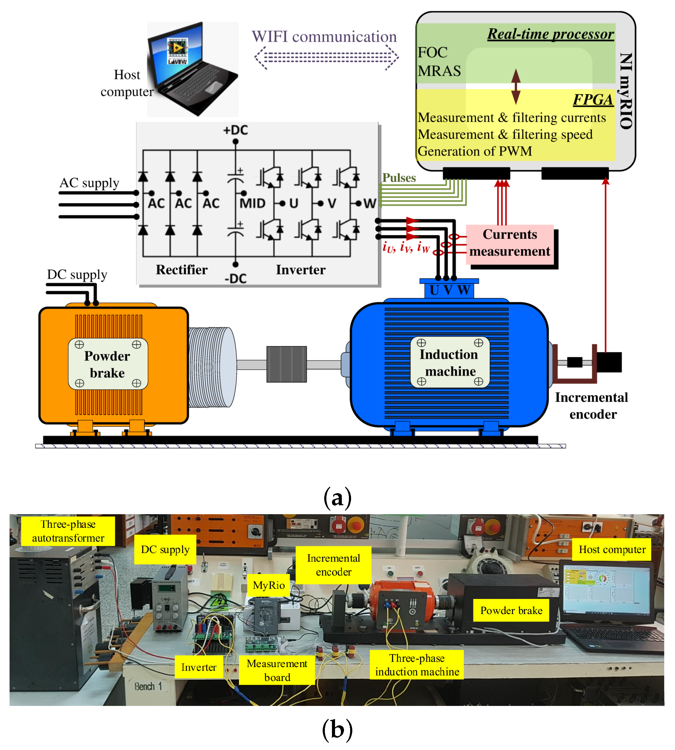
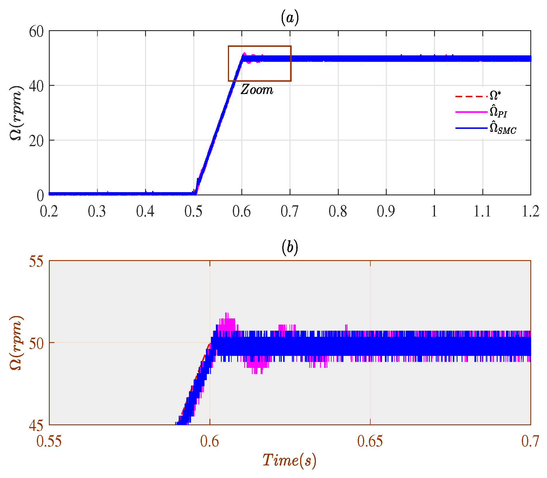
4. Experimental Validation

Simulation studies have been validated on a MyRio platform based on a closed-loop control system of a three-phase induction machine laboratory setup. The data recording, instrumentation, and parameters tuning have been performed using LabVIEW systems engineering software. The parameters used in the implementation tests are presented in Table 1.
The control algorithm is realized by developing two programs: the first one targeting the configuration of the MyRio-FPGA for measurement-filtering of currents, measurement-filtering the mechanical speed and generation of PWM signals, while the second program is realized for real-time (RT) processor in order to create the FOC based on measurement speed- and SFOC-based estimated speed. When running the control system, a bidirectional flow of data is present between the RT program and the FPGA program. Figure 12 shows the illustration and real photograph of the test bench.
FOC and MRAS have been programmed in timed-loop that is executed every T s = 150 μs to ensure the essential control procedures, which are strictly time dependent. The timed-loop includes flat sequence structure, which is divided into three required parts as follows:
  • Measurement of signals, computations, and transformations;
  • FOC structure with PI controllers and MRAS estimator; and
  • Application of the calculated control signals.
All of the integrations or derivations required in FOC algorithm and MRAS estimator have been performed using shift register. In order to ensure a fair performance comparison between the two control algorithms under different operating conditions, it is important to ensure initially the same performances under the normal inertia operating condition. To achieve this goal according to the calculation performed in the last section, the sliding mode and PI controller parameters were set to be equal the values calculated in simulation.
The implementation section is divided into two parts: the first part is focused on the use of the FOC, while the second part deals with the use of the SFOC based on the MRAS-PI and the MRAS-SMC.

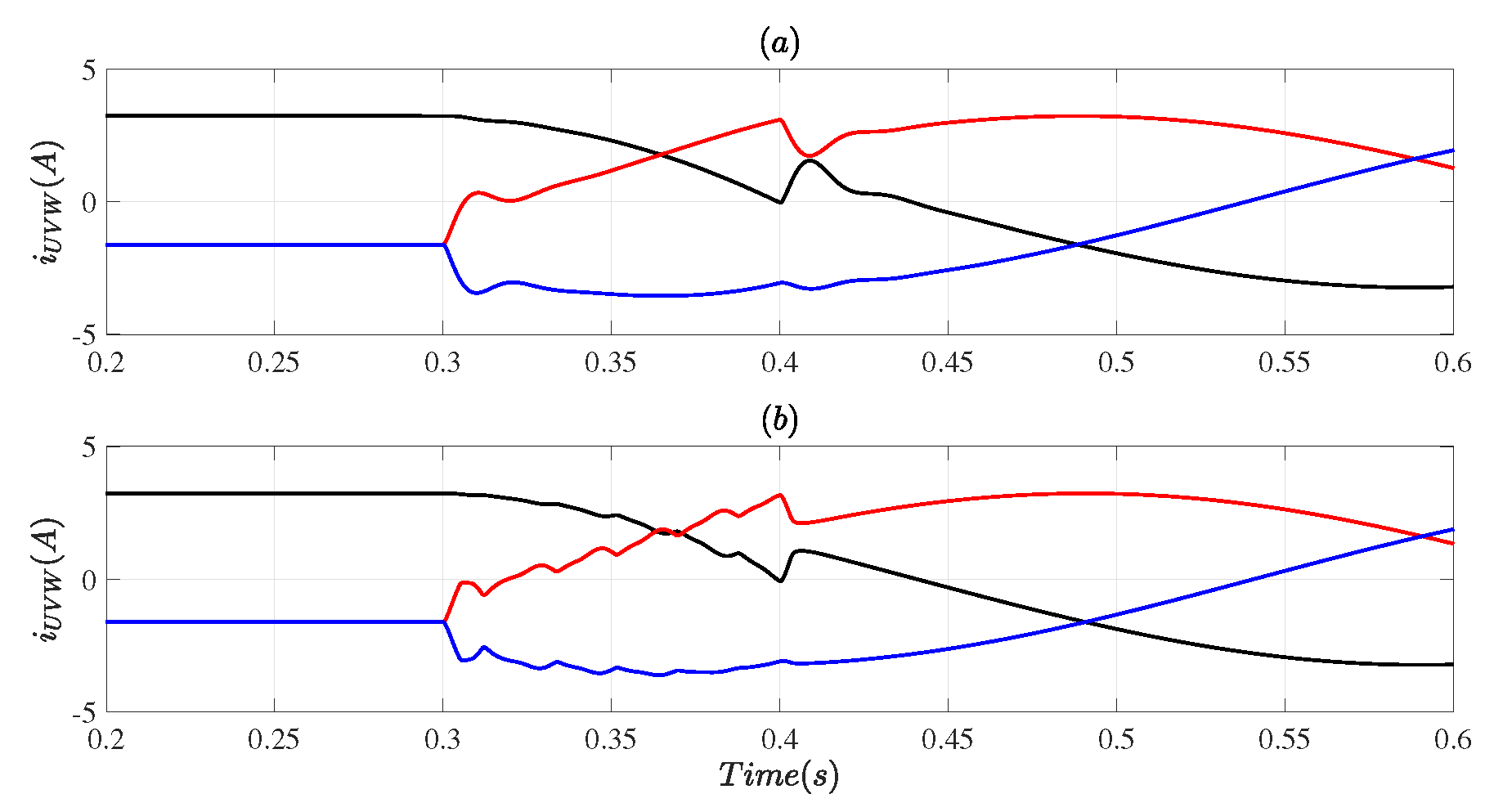
4.1. Closed-Loop Using Measured Speed

In order to obtain similar performances to those obtained when using the measured speed in the control-loop; the MRAS-PI and MRAS-SMC have been simulated simultaneously with the FOC using the measured speed. The obtained results under normal inertia operating condition are shown in Figure 13 and Figure 14, while those obtained during modified inertia are shown in Figure 15 and Figure 16.
It is obvious form the results shown in Figure 13 and Figure 14 that the use of the MRAS-PI and the MRAS-SMC gives similar performances under normal inertia operating condition. However, when the inertia has been changed during the operation mode, the obtained performance with the use of the MRAS-PI was slightly degraded in tracking the reference with the presence of overshoots of 6% and 2% for low and high speed ranges, respectively.

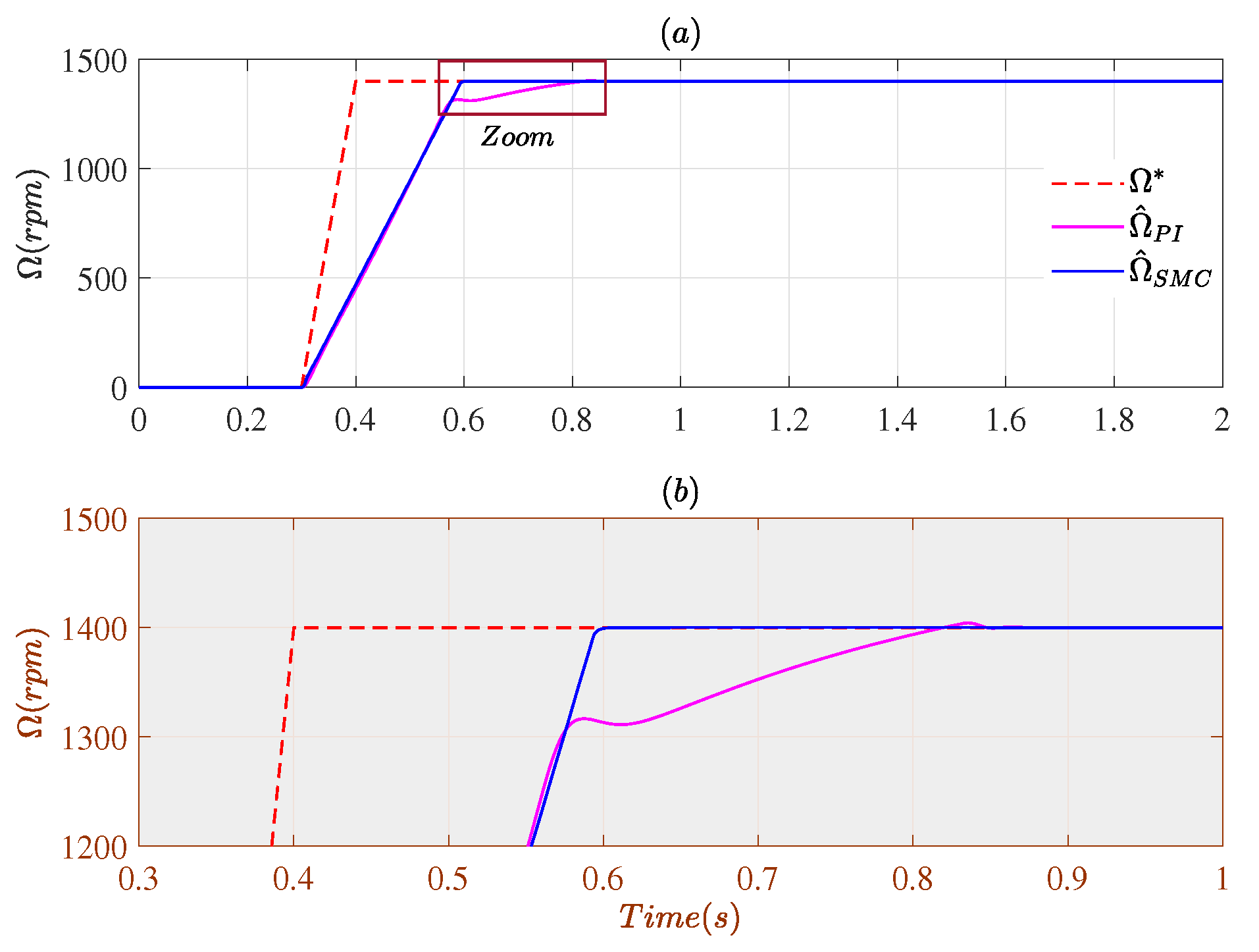
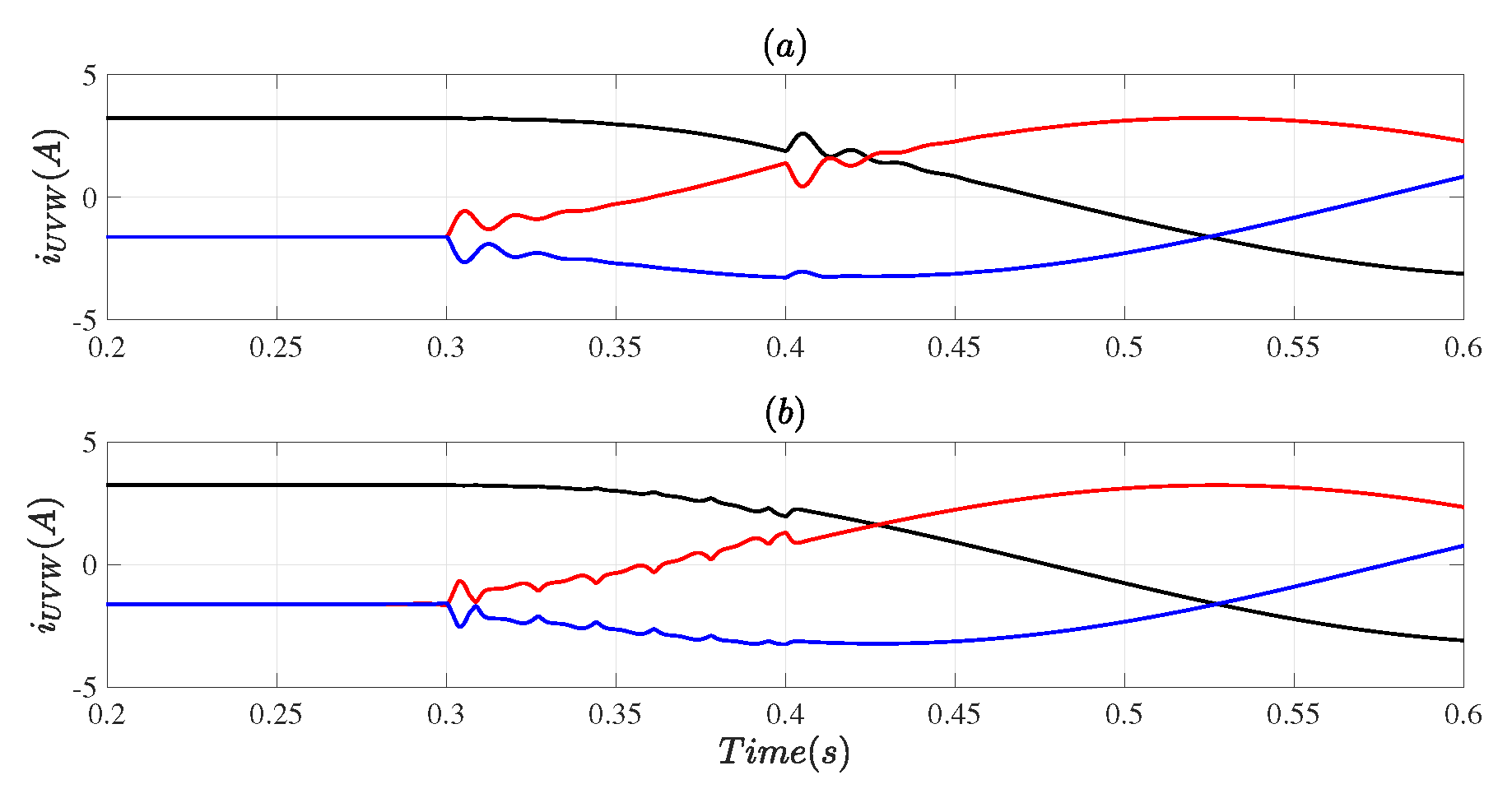
4.2. Closed-Loop Using Estimated Speeds

In this part, the SFOC is applied using the MRAS-PI and the MRAS-SMC under varying inertia and for different speed ranges. The obtained results are shown in the same figure. Figure 17 and Figure 18 show the obtained results for the application of the SFOC using MRAS-PI and MRAS-SMC at normal inertia conditions for low and high ranges of speed, while Figure 19 and Figure 20 show the obtained results under varying inertia operation mode.
Figure 18a and its zoom Figure 18b, show an overall performance degradation of the SFOC using MRAS-PI in ranges of high speed. It is obvious that the performance degradation becomes more important when the inertia changes, as shown clearly in Figure 20a,b. On the other hand, in the ranges of low speed, the obtained results of the SFOC using MRAS-PI present good performance in both cases, under nominal and modified inertia as shown clearly in Figure 17 and Figure 19. In contrast, Figure 17, Figure 18, Figure 19 and Figure 20 show the good performance of the SFOC when using MRAS-SMC for all tests and under different operating conditions where these obtained performances are similar to those obtained for the FOC using the measured speed.

5. Conclusions

The selection of a large range of reference speeds and the inertia variation affect the transient performance of the sensorless field-oriented control (SFOC) for induction motors (IM). In order to overcome this issue, this paper presented a new design of switching linear feedback sliding mode controller (SLF-SMC) for a model reference adaptive system (MRAS). The simulation and implementation studies, performed under different speed ranges and operation conditions such as a variation of the inertia, showed that the dynamic performance of the sensorless Field oriented control (SFOC) using MRAS-SMC is higher than that obtained when using MRAS-PI. Indeed, the performance of the SFOC using the MRAS-PI presented a clear deterioration at high speeds under normal and modified inertia conditions, unlike the SFOC using MRAS-SMC, which maintained a good performance similar to that obtained with FOC for all speed ranges. The design of the time-varying sliding mode control for MRAS could be a good extension for this research.

Supplementary Materials

The project source codes are available at https://github.com/MohamedAmineFnaiech/MRAS_SMC_SLF.

Author Contributions

Conceptualization, M.A.F.; Funding acquisition, J.G.; Investigation, M.A.F.; Methodology, M.A.F.; Software, M.A.F.; Validation, M.A.F.; Writing—original draft, M.A.F.; Writing—review and editing, J.G., M.T., A.K., M.B. and K.L. All authors have read and agreed to the published version of the manuscript.

Funding

Publication was supported by Gdansk University of Technology.

Conflicts of Interest

The authors declare no conflict of interest.

Abbreviations

The following abbreviations are used in this manuscript:
IMInduction machine
FOCField-oriented control
SFOCSensorless field-oreinted control
MRASModel reference adaptive system
SMCSliding-mode control
PIProportional-integral controller
SLFSwitching linear feedback

Nomenclature

R r Rotor resistance
L r Rotor inductance
L s Stator inductance
L m Main inductance
λ = R r L r Inverse of rotor time constant
σ = 1 L m 2 L s L r Total leakage factor
v s u , v s v , v s w u-v-w Stator voltage components
v s α , v s β α - β Stator voltage components
i s u , i s v , i s w u-v-w Stator current components
i s α , i s β α - β Stator current components
i s d , i s q d-q Stator current components
ψ s α , ψ s β α - β Stator flux components
ψ r α , ψ r β α - β Rotor flux components
ω r Rotor electrical angular speed
SSwitching surface
sLaplace variable
ω s l Slip angular speed
PNumber of pole pairs
Ω Rotor mechanical shaft speed
. * Desired value
. ^ Estimated value
P A R K PARK transformation
P A R K 1 Inverse of PARK transformation
θ s Angle of PARK transformation

References

  1. Guzinski, J.; Abu-Rub, H. Speed sensorless induction motor drive with predictive current controller. IEEE Trans. Ind. Electron. 2013, 60, 699–709. [Google Scholar] [CrossRef]
  2. Schauder, C. Adaptive speed identification for vector control of induction motors without rotational transducers. IEEE Trans. Ind. Appl. 1992, 28, 1054–1061. [Google Scholar] [CrossRef]
  3. Kojabadi, H.; Liuchen, C.; Doraiswami, R. A mras-based adaptive pseudoreduced-order flux observer for sensorless induction motor drives. IEEE Trans. Power Electron. 2005, 20, 930–938. [Google Scholar] [CrossRef]
  4. Gadoue, S.; Giaouris, D.; Finch, J. Mras sensorless vector control of an induction motor using new sliding-mode and fuzzy-logic adaptation mechanisms. IEEE Trans. Energy Convers. 2010, 25, 394–402. [Google Scholar] [CrossRef]
  5. Comanescu, M.; Xu, L. Sliding-mode mras speed estimators for sensorless vector control of induction machine. IEEE Trans. Ind. Electron. 2006, 53, 146–153. [Google Scholar] [CrossRef]
  6. Cirrincione, M.; Accetta, A.; Pucci, M.; Vitale, G. Mras speed observer for high-performance linear induction motor drives based on linear neural networks. IEEE Trans. Power Electron. 2013, 28, 123–134. [Google Scholar] [CrossRef]
  7. Zbede, Y.B.; Gadoue, S.M.; Atkinson, D.J. Model predictive mras estimator for sensorless induction motor drives. IEEE Trans. Ind. Electron. 2016, 63, 3511–3521. [Google Scholar] [CrossRef] [Green Version]
  8. Dominguez, J.R. Discrete-time modeling and control of induction motors by means of variational integrators and sliding modespart ii: Control design. IEEE Trans. Ind. Electron. 2015, 62, 6183–6193. [Google Scholar] [CrossRef]
  9. Hung, J.C.; Gao, W. Variable structure control: A survey. IEEE TTrans. Ind. Electron. 1993, 40, 2–21. [Google Scholar] [CrossRef] [Green Version]
  10. Levant, A. Principles of 2-sliding mode design. Automtica 2007, 43, 576–586. [Google Scholar] [CrossRef] [Green Version]
  11. Holakooie, M.; Ojaghi, M.; Taheri, A. Modified dtc of a six-phase induction motor with a second-order sliding-mode mras-based speed estimator. IEEE Trans. Power Electron. 2019, 34, 600–611. [Google Scholar] [CrossRef]
  12. Wang, H.; Ge, X.; Liu, Y. Second-order sliding-mode mras observerbased sensorless vector control of linear induction motor drives for medium-low speed maglev applications. IEEE Trans. Ind. Electron. 2018, 65, 9938–9952. [Google Scholar] [CrossRef]
  13. Tarchala, G.; Orlowska-Kowalska, T. Equivalent-signal-based sliding mode speed mras-type estimator for induction motor drive stable in the regenerating mode. IEEE Trans. Ind. Electron. 2018, 65, 6936–6947. [Google Scholar] [CrossRef]
  14. Benlaloui, I.; Drid, S.; Chrifi-Alaoui, L.; Ouriagli, M. Implementation of a new mras speed sensorless vector control of induction machine. IEEE Trans. Energy Convers. 2015, 30, 588–595. [Google Scholar] [CrossRef]
  15. Utkin, V. Discussion aspects of high-order sliding mode control. IEEE Trans. Autom. Control. 2016, 61, 829–833. [Google Scholar] [CrossRef]
  16. Zhao, Z.; Gu, H.; Zhang, J.; Ding, G. Terminal sliding mode control based on super-twisting algorithm. J. Syst. Eng. Electron. 2017, 28, 145–150. [Google Scholar] [CrossRef]
  17. Ding, S.; Wang, J.; Zheng, W.X. Second-order sliding mode control for nonlinear uncertain systems bounded by positive functions. IEEE Trans. Ind. Electron. 2015, 62, 5899–5909. [Google Scholar] [CrossRef]
  18. Abu-Rub, H.; Iqbal, A.; Guzinski, J. High Performance Control of AC Drives with Matlab/Simulink Models; A John Wiley & Sons: Hoboken, NJ, USA, 2012. [Google Scholar]
  19. Davari, S.A.; Wang, F.; Kennel, R.M. Robust deadbeat control of an induction motor by stable mras speed and stator estimation. IEEE Trans. Ind. Inform. 2018, 14, 200–209. [Google Scholar] [CrossRef]
  20. Das, S.; Kumar, R.; Pal, A. Mras-based speed estimation of induction motor drive utilizing machines’ d- and q-circuit impedances. IEEE Trans. Ind. Electron. 2019, 66, 4286–4295. [Google Scholar] [CrossRef]
  21. Cao, P.; Zhang, X.; Yang, S. A unified-model-based analysis of mras for online rotor time constant estimation in an induction motor drive. IEEE Trans. Ind. Electron. 2017, 64, 4361–4371. [Google Scholar] [CrossRef]
  22. Popov, V.M. Hyperstability of Control Systems; Springer: Berlin/Heidelberg, Germany, 1973. [Google Scholar]
  23. Pal, A.; Das, S.; Chattopadhyay, A. An improved rotor flux space vector based mras for field-oriented control of induction motor drives. IEEE Trans. Power Electron. 2018, 33, 5131–5141. [Google Scholar] [CrossRef]
  24. Dehghan-Azad, E.; Gadoue, S.; Atkinson, D.; Slater, H.; Barrass, P.; Blaabjerg, F. Sensorless control of im based on stator-voltage mras for limp-home ev applications. IEEE Trans. Power Electron. 2018, 33, 1911–1921. [Google Scholar] [CrossRef]
  25. Accetta, A.; Cirrincione, M.; Pucci, M.; Vitale, G. Closed-loop mras speed observer for linear induction motor drives. IEEE Trans. Ind. Appl. 2015, 51, 2279–2290. [Google Scholar] [CrossRef]
  26. Utkin, V.I. Sliding Mode Control in Discrete-Time and Difference Systems; Springer: Berlin/Heidelberg, Germany, 1994. [Google Scholar]
  27. Fnaiech, M.A.; Trabelsi, M.; Khalil, S.; Mansouri, M.; Nounou, H.; Abu-Rub, H. Robust sliding mode control for three-phase rectifier supplied by non-ideal voltage. Control Eng. Pract. 2018, 77, 73–85. [Google Scholar] [CrossRef]
  28. Huber, O.; Acary, V.; Brogliato, B. Lyapunov stability and performance analysis of the implicit discrete sliding mode control. IEEE Trans. Autom. Control 2016, 61, 3016–3030. [Google Scholar] [CrossRef] [Green Version]
Figure 1. Design and mathematical concept of the MRAS estimator.
Energies 14 03083 g001
Figure 2. Block diagram of the proposed MRAS-based Switching Linear Feedback technique.
Energies 14 03083 g002
Figure 3. Phase plan for negative and positive feedback: (a) spiral and (b) hyperbolas.
Energies 14 03083 g003
Figure 4. Performance indices for different speeds: (a) nominal inertia condition and (b) modified inertia condition.
Energies 14 03083 g004
Figure 5. SFOC using MRAS-based SMC-SLF.
Energies 14 03083 g005
Figure 6. Control of the estimated speeds at low ranges with the nominal inertia condition. (a) Desired and estimated speeds. (b) Zoom.
Energies 14 03083 g006
Figure 7. Control of the estimated speeds at high ranges with the nominal inertia condition. (a) Desired and estimated speeds. (b) Zoom.
Energies 14 03083 g007
Figure 8. Control of the estimated speeds at low ranges when varying inertia. (a) Desired and estimated speeds. (b) Zoom.
Energies 14 03083 g008
Figure 9. Control of the estimated speeds at high ranges when varying inertia. (a) Desired and estimated speeds. (b) Zoom.
Energies 14 03083 g009
Figure 10. Stator currents at low ranges of speed with the nominal inertia condition. (a) PI (b) SMC-SLF.
Energies 14 03083 g010
Figure 11. Stator currents at low ranges of speed when varying inertia. (a) PI (b) SMC-SLF.
Energies 14 03083 g011
Figure 12. (a) Illustration of the test bench, (b) real photograph of a test bench.
Energies 14 03083 g012
Figure 13. Implementation using measured speed at low speeds when using the nominal inertia condition. (a) Desired, measured, and estimated. (b) Norm of flux error.
Energies 14 03083 g013
Figure 14. Implementation using measured speed at high speeds when using the nominal inertia condition. (a) Desired, measured, and estimated. (b) Norm of flux error.
Energies 14 03083 g014
Figure 15. Implementation using measured speeds at low speed when using modified inertia condition. (a) Desired, measured, and estimated. (b) Zoom. (c) Norm of flux error.
Energies 14 03083 g015
Figure 16. Implementation using measured speed at high speeds when using the modified inertia condition. (a) Desired, measured, and estimated. (b) Zoom. (c) Norm of flux error.
Energies 14 03083 g016
Figure 17. Implementation using estimated speed at low speeds when using the nominal inertia condition. (a) Desired and estimated speeds. (b) Zoom.
Energies 14 03083 g017
Figure 18. Implementation using estimated speed at high speeds when using the nominal inertia condition. (a) Desired and estimated speeds. (b) Zoom.
Energies 14 03083 g018
Figure 19. Implementation using estimated speed at low speeds when using the modified inertia condition. (a) Desired and estimated speeds. (b) Zoom.
Energies 14 03083 g019
Figure 20. Implementation using estimated speed at high speeds when using the modified inertia condition. (a) Desired and estimated speeds. (b) Zoom.
Energies 14 03083 g020
Table 1. Specification of the test bench.
Induction Motor Nominal Parameters
DescriptionParameterValue
Power P N 1.5 kW
Voltage U N 3 × 400 V 50 Hz
Current I N 3.5 A
Speed n N 1410 rpm
Efficiency η N 0.79
Power coefficient c o s φ n 0.78
Torque T N 10.16 Nm
Stator resistance R s 4.74 Ω
Rotor resistance R r 4.75 Ω
Mutual inductance L m 303 mH
Stator inductance L s 320 mH
Rotor inductance L r 320 mH
Inertia J n 0.0038 kg m 2
Modified inertia J n 0.007 kg m 2
Inverter nominal parameters
Power P N 6.1 kW
Voltage U N 3 × 420 V 50 Hz
Current I N 7.5 A
Switching frequency f s w 30 kHz
DC Voltage V d c 600 V
Publisher’s Note: MDPI stays neutral with regard to jurisdictional claims in published maps and institutional affiliations.

