Abstract
The article presents a method for solving the inverse problem of a two-dimensional anomalous diffusion equation with a Riemann–Liouville fractional-order derivative. In the first part of the present study, the authors present a numerical solution of the direct problem. For this purpose, a differential scheme was developed based on the alternating direction implicit method. The presented method was accompanied by examples illustrating its accuracy. The second part of the study concerned the inverse problem of recreating the model parameters, including the orders of the fractional derivative, in the anomalous diffusion equation. Equations of this type can be used to describe, inter alia, the heat conductivity in porous materials. The ant colony optimization algorithm was used to solve this problem. The authors investigated the impact of the distribution of measurement points, the use of different mesh sizes, and the input data errors on the obtained results.
1. Introduction
In recent years, derivatives of fractional order have been frequently used. Many different definitions of such derivatives are available in the literature. In applications, the Caputo derivative and the Riemann–Liouville derivative are the most often used [1,2]. Fractional calculus is used, inter alia, in mathematical modeling of various problems in mechanics, physics, and biology [3,4,5,6], in control theory [7], in image processing [8], as well as in modeling the phenomena of heat transport [9,10,11,12,13,14,15]. Many mathematical models are based on differential equations containing fractional derivatives. Hence, the development of algorithms for solving differential equations with fractional derivatives is extremely important [16,17,18,19,20]. For example, in [16], the authors presented a solution of fractional pantograph differential equations. They used the operational matrix of the derivatives of the generalized Lucas polynomials and then transformed the problem into a system of equations. The paper also included the derivation of the numerical scheme with examples.
Direct problems for differential equations consist of solving a given equation (determining the state function) when all input data are known. Solving inverse problems, on the other hand, involves determining some of the input data on the basis of some information regarding the state function. In the literature, studies on inverse problems for differential equations with fractional derivatives are available. The first studies on these issues were by Murio [21,22]. In these papers, the one-dimensional problem was considered, and the mollification method was used to solve it. Zheng and Wei [23,24] presented a Fourier regularization and a convolution methods to recreate the boundary condition (function and its derivative) of a semi-infinite domain for the time-fractional inverse advection-dispersion equation. A similar issue is considered in the finite domain in [25], in this case a kernel-based meshless method was used. Xiong et al. [26] considered a two-dimensional case in the infinite domain. Yan and Yang [27] used an efficient Kansa-type method and presented numerical solution of two-dimensional time-fractional inverse diffusion problems. For the theoretical results of the stability and the uniqueness of the solution, a backward problem and inverse source problem for a multi-dimensional time-fractional diffusion equation were included in [28]. The authors of [29,30] managed the inverse problem for the two-dimensional time-fractional sideways heat equation in the infinite domain. Inverse problems for two-dimensional time-fractional diffusion equation were also considered in [29,31,32,33]. The study [34] considered the inverse problem for two-dimensional fractional partial differential equations. The method assumes the knowledge of the state function for a certain time interval at each point of the domain under consideration. A hybrid method based on modulating functions was used for the solution. The inverse problem for the heat equation in the two-dimensional domain with the Atangana–Baleanu fractional derivative was considered in [35]. In turn, the equation with the Hilfer derivative was considered in [36].
Research on one-dimensional issues prevails in the literature. Those on two-dimensional problems mainly regard the Caputo derivative in an infinite domain. There are a few articles on the inverse problem for the two-dimensional anomalous diffusion equation with the Riemann–Liouville derivative. Furthermore, the artificial intelligence algorithm was used in only one study in relation to time-fractional Schrödinger equations. The authors of this manuscript considered this rarely described case.
One of the main problems with using models with the fractional derivative is determining the order of the derivative. There are papers in which the authors determined it based on physical experiments [37]. To determine the order of the derivative, it may be useful to solve the inverse problem, which the authors present in this paper.
The article presents the consideration of the inverse problem for a two-dimensional anomalous diffusion equation with the Riemann–Liouville fractional derivative. The inverse problem in the study was to recreate the orders of two fractional derivatives and one of the parameters in the equation. Additional information, in this case, was the solution values at selected points of the domain. To solve the inverse problem, the direct problem should be repeatedly solved for the fixed values of the searched parameters. To solve the direct problem, the alternating direction implicit method was used [38], which allows for solving of multidimensional problem by the iterative solution of a number of one-dimensional problems. Using the given values of the solution and the values determined from the solution of the direct problem, a functional representing the error of the approximate solution was built. The argument for which the functional reached the minimum value was the sought solution for the inverse problem under consideration. The minimum of the functional was searched for using the ant colony optimization algorithm [39,40]. This is a probabilistic artificial intelligence algorithm inspired by the behavior of an ant colony. The authors of the study investigated the impact of the distribution of measurement points, the use of different mesh sizes, and the value of input data disturbances on the obtained results.
2. Space Fractional Diffusion Equation
The presented model in this section can be used to describe heat flow in a porous material with an irregular (fractal, chaotic) structure. In such a case, the heat flow can be modeled using fractional-order derivatives [10]. We considered a two-dimensional problem in which the derivative over space was a Riemann–Liouville type. Thus, the study considered the two-dimensional space fractional diffusion equation with the Riemann–Liouville derivative:
specified in the following area , where and . Initial-boundary conditions were attached to the above equation:
It was also assumed that both constants and functions are positive for all . Equation (1) describes the phenomenon of anomalous diffusion, for example the phenomenon of heat conduction in porous materials [9,10,11]. In Equation (1), both the right- and left-hand Riemann–Liouville derivatives were used as fractional derivatives relative to space [1,2]:
where . Similar to the formula (3), we can define the fractional derivatives for a variable y and order .
Considering Equation (1) with the conditions (2) as a model describing the heat conductivity in porous materials, the following notations can be assumed:
- —heat conductivity coefficients,
- c—specific heat of a medium,
- —density of a medium,
- u—a function describing the temperature distribution in space and time,
- f—an additional heat source.
3. Direct Problem
In this section, we present a way of solving Equation (1) numerically, and then, we introduce an example illustrating the accuracy of the method. For the discretization of the equation, the finite difference method supplemented with the appropriate discretization of Riemann–Liouville was used.
3.1. Numerical Method
Equation (1) can be written as follows:
We commence with the discretization of the domain . For this purpose, we introduce the following notations: , , , , , , , , , where , and are the mesh points. Using , we denote the function values, respectively, , and in points .
We approximate the Riemann–Liouville derivative as follows [41] (the order of approximation ):
where:
The formulas for the fractional derivative with respect to the variable y look similar. The derivative with respect to time is approximated as follows (the order ):
For simplicity, we introduce the following notation:
The approximation formulas for the derivative of the variable y are analogous. Then, the difference scheme of the order for Equation (4) takes the form:
After transforming the above equation, we can write:
for , and .
We write the above difference scheme in matrix form. For this purpose, we define two matrices:
where:
The next step is to define block matrices S and H. We start with the matrix S (dimension ), which is a diagonal block matrix, i.e., it contains matrices on the main diagonal and zeros in other places.
Below is the form of matrix H (matrix H has the same dimension as matrix S). Matrix H is a block matrix where each block is a diagonal matrix of dimension .
The matrices appearing in the difference scheme (20) are quite large; as a consequence, the resulting system of equations will be time consuming to solve, which is shown in Section 3.2. Hence, we applied the alternating direction implicit method (ADIM) to the difference scheme (15), which significantly reduces the computation time. This will be an important issue in the case of solving the inverse problem, in which direct problem should be solved repeatedly. We write the scheme (15) in the form of the directional separation product:
Then, the above scheme can be broken in two parts and solved, respectively, first in direction x and, afterwards, in direction y. As a consequence, the resulting matrices for the system of equations will have significantly lower dimensions than in the case of the scheme (15). The solution algorithm consists of two successive steps:
- for each fixed , we solve the scheme in the direction x. As a result, we obtain a temporary solution :
- then, for each fixed , we solve the scheme in direction y:
We can represent this process symbolically by means of Figure 1. For the boundary nodes and the initial condition, we assumed:
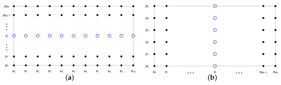
Figure 1.
Numerical solution in the horizontal direction (for a fixed node ) (a) and the vertical direction (for a fixed node ) (b).
Furthermore, for the ADIM method, we write the appropriate matrix equations. First, for each , we define auxiliary vectors :
where . Hence, we obtain an auxiliary matrix of dimension . Then, the scheme (22) can be written in the following matrix form (for ):
where the temporary solution takes the form , and , . In this step, we solved systems of equations, each of dimension. Afterwards, we present the scheme (23) in direction y in matrix form (for ):
where and . From this step of the algorithm, we solved systems of equations with dimensions each. The Bi-CGSTAB [42,43] method was used to solve the equation systems, which also influenced the computation time. A comparison with the Gauss algorithm is presented in the next section. The proof of the convergence of the above difference schemes can be found in [38].
3.2. Numerical Results
In this section, we present the results of the numerical solution of the problem (1) and (2). The example assumes the following data:
For the data defined above, the exact solution (1) and (2) is the function:
where the domain under consideration is as follows: .
Errors are marked as follows:
where , and denotes exact values of the function u at the mesh points. First of all, we compared the results obtained with and without the ADIM for different meshes. We also provided computation times. As can be seen in Table 1, the results obtained with or without ADIM were similar; the differences were slight. However, the difference in the computation time was of considerable size; for example, for the mesh , in the case of the ADIM, this time was about 9 s, while for the method without ADIM, this time was about 453 s. The difference was enormous, and considering that in the inverse problem, it is necessary to solve the direct problem repeatedly, the use of ADIM was essential.

Table 1.
Comparison of the results and the times of the algorithm computation depending on the use of ADIM.
Another important issue influencing the computation time was the appropriate selection of the method to solve the system of equations. In the presented algorithm, the Bi-CGSTAB method [42,43] was used to solve a system of linear equations. We compared the computation times of the algorithm in the case of using Bi-CGSTAB and the Gaussian elimination method (Table 2). In the case of mesh , the use of the Bi-CGSTAB caused the computation to be performed approximately times faster than using the Gaussian elimination method.
Table 2.
Comparison of the algorithm computation times depending on the method used to solve the system of equations.
4. Inverse Problem
In this section, we present a solution of the inverse problem involving the reconstruction of the selected parameters of the model described by Equation (1). The considered inverse problem consisted of selecting the unknown input parameters of the model in such a way that the model output (function u from Equation (1)) had predetermined values at selected points of the domain. A lack of information regarding the searched input parameters was compensated by the values of the function u at selected points of the domain. Due to the fact that the inverse problems are ill-conditioned, they are classified as quite difficult issues.
4.1. Formulation of the Problem
We considered the following equation:
where:
and function is given by the formula (27). We considered the differential equation in the domain , where . The unknown parameters of the model that should be determined were . However, the values of the function u at selected points of the domain were known. In order to test the stability of the algorithm, we considered:
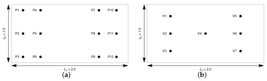 Figure 2. Two different arrangements of the measuring points.
- three types of meshes (): , , and ;
- different types of measurement data disturbances (errors with a normal distribution): .
In order to reconstruct the unknown parameters , we developed a functional comparing the values of the numerical solution depending on the parameters sought with the measurement data :
where is the number of measurement points, and is the number of measurements. The values are obtained from the solution of the direct problem for fixed parameter values .
4.2. Objective Function Minimization
In order to find minimum of the objective function (28), and then solve inverse problem, the Ant Colony Optimization (ACO) algorithm was used [39,40]. The ACO algorithm is inspired by behavior of an ant colony in nature. In the considered version of the algorithm, solutions, which in our case were vectors, are treated as the so-called pheromone spots. In the initial phase of the algorithm, these spots are randomly distributed in the considered domain. Then, they are sorted by quality, and each solution (pheromone spot) is assigned a probability of choice. The better the solution is, the higher the probability is. The probability is determined on the basis of the quality of the solution and the q parameter of the algorithm, which we can control. In the case of a low q, the best solution is preferred, and as q increases, the probability of choosing any solution becomes similar. As a result, we obtained an ordered set of solutions. Then, the iterative phase of the algorithm begins, in which each ant (which are M) selects a spot according to its probability and then transforms it to sample the neighborhood. In the considered algorithm, to transform the solution, we used the Gaussian distribution density function. As a result of the transformation, we obtained M new solutions (pheromone spots). Next, the solution set must be updated with new pheromone spots (solutions) by sorting all solutions according to quality, and then, M the worst solutions are deleted. We repeated the iterative process I times. Finally, we chose the best solution. The algorithm was adapted to parallel computations. A more detailed description of the algorithm can be found in [9].
5. Results
In the considered inverse problem, we determined the parameters . The exact values of these parameters were respectively . As we mentioned earlier, to test the stability of the algorithm, we assumed different arrangements of the measurement points, mesh sizes, and input data disturbances. For example, in Figure 3, we can see a comparison of the input data not disturbed by the error and disturbed by the error from the measurement point .
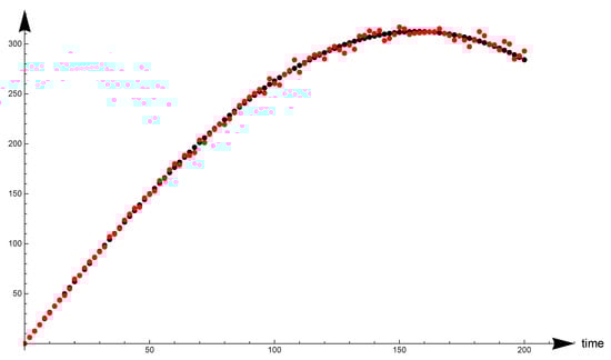
Figure 3.
Disturbed (red dots) and exact (black dots) values of the function u at measuring point (disturbed with the error ).
The following parameter values were adopted in the ant algorithm:
Due to the probabilistic nature of the ant algorithm, we assumed five runs for the given settings, and then, the best one was selected from the obtained results. For this reason, in the tables with the results, the value of the standard deviation for the obtained values of the objective function was added. As can be seen, they were inconsiderable, which proved that the algorithm gave very similar results each time.
Table 3 shows the results of reconstructing the searched parameters for various meshes and the values of input data disturbances in the case of twelve measurement points. In each case, the errors of the results obtained were low and did not exceed . For the input data without error, the results were the best. Even with disturbance of the input data, the obtained results were satisfying, which proved the stability of the model and algorithm. Table 4 contains analogous data for the case of seven measuring points. As can be seen, the change in the arrangement of measurement points, as well as their number influenced the obtained results. In a few cases (for example, for the mesh and disturbance), the errors in recreating selected parameters exceeded , which did not happen in the case of twelve measuring points. It can therefore be concluded that the arrangement of the measuring points and their number had a significant impact on the results. At the same time, it should be noted that also in this case, the obtained errors of the reconstruction coefficient were at a satisfactory level. Only in five cases, the recreating error exceeded .
Table 3.
Results of the calculations in the case of twelve measurements points ): —reconstructed value of x-directional order derivative , —reconstructed value of y-directional order derivative , —reconstructed value of parameter c, —relative error of reconstruction, J—value of the objective function, —standard deviation of the objective function.
Table 4.
Results of calculations in the case of seven measurements points ): —reconstructed value of x-directional order derivative , —reconstructed value of y-directional order derivative , —reconstructed value of parameter c, —relative error of reconstruction, J—value of the objective function, —standard deviation of the objective function.
We next verified the errors of the recreating function u in the measuring points for the recreated parameters . In all cases, these errors were at a low level. A tendency can be seen that as input data noise increased, the recreating errors of the function u increased, although this was not always the case. A similar tendency applied to the mesh density; in general, the lowest reconstruction errors were obtained for the mesh and the highest for the mesh. Importantly, the average errors of the recreating function u turned out to be greater for the second arrangement of measurement points (seven measurement points) in ten of twelve cases (see Table 5 and Table 6).
Table 5.
Errors of reconstruction function u in measurement points for twelve measurement points (—average absolute error, —maximum absolute error, —average relative error, —maximum relative error).
Table 6.
Errors of reconstruction function u in measurement points for seven measurement points (—average absolute error, —maximum absolute error, —average relative error, —maximum relative error).
Figure 4 and Figure 5 show the distribution of the reconstruction errors of the function u at selected points of the domain ( and ) for the mesh. The greater the noise on the input data was, the greater these errors were. For exact data, the reconstruction errors were at a stable, low level. In the case of point , it can be seen that the reconstruction error for input data disturbed with a noise error at the end of the process was greater than the corresponding error for a noise of .
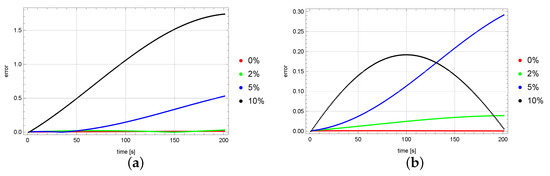
Figure 4.
Errors in measurement points (a) and (b) in the case of a mesh size.
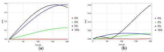
Figure 5.
Errors in measurement points (a) and (b) in the case of a mesh size.
Now, we present a way of achieving the solution by the ACO algorithm. Figure 6 and Figure 7 show the values of the objective function in successive iterations of the algorithm for the case of the mesh, seven measurement points, and various input data noise values. The values of the objective function for the first few iterations were relatively high; therefore, due to the scale, they are not marked in the figures. It can be seen that around 15 iterations, these values stabilized, and in the last iterations, the algorithm slightly improved the searched minimum. The selection of the parameters for the ant algorithm is quite important and was obtained based on the experience of the authors [40,44].
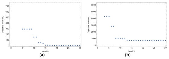
Figure 6.
Values of the objective function in the case of (a) and (b) perturbation of the input data.
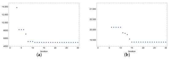
Figure 7.
Values of the objective function in the case of (a) and (b) perturbation of the input data.
Finally, we present the influence of the recreated parameters on the values of the function u at the measuring point . For this purpose, we calculated the values of the function u at the point for different values of the parameters . Firstly, we determined the values of the parameters , and we changed the values of the parameter . Then, we similarly executed with the parameter at fixed values of the . Finally, we set the parameters, and the parameter c took the values . As can be seen in Figure 8, Figure 9 and Figure 10, a change in the value of the parameter had a greater impact on the obtained values of the function u at point than in the case of the derivative order. Furthermore, introducing a change in the value of the parameter c had a significant impact on the function, especially in the case of lower values of the parameter c. It can also be observed that changing the derivative parameter affected the u function to a lesser extent than the other parameters.
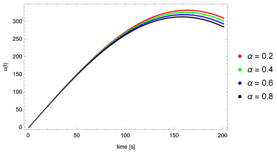
Figure 8.
Values of the function u at point for different values of the parameter ().
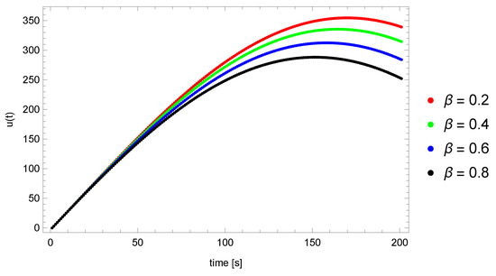
Figure 9.
Values of the function u at point for different values of the parameter ().
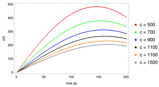
Figure 10.
Values of the function u at point for different values of the parameter c ().
6. Conclusions
The paper presented a numerical solution of a two-dimensional differential equation with a fractional derivative with respect to a space of the Riemann–Liouville type. This type of equation can describe the phenomenon of heat conduction in porous media, which the authors will also consider in further research. The presented numerical solution was also used to solve the inverse problem consisting of recreating the orders of the derivatives and the parameter c. The presented results of the numerical experiment seemed satisfactory, and the algorithm was stable even for input data burdened with noise (measurement error).
The presented algorithm was characterized by faster calculations in relation to the classic differential scheme, resistance to falling into local minima compared to other minimization methods, low requirements for the objective function (it was not necessary to require continuity, differentiability, or convexity), and the stability against input data errors. The above-described properties can be treated as its advantages. The only downside was the computation time of the ACO algorithm.
In the further part of the research, the authors plan the following:
- continued tests of the proposed algorithm (reconstructing of more parameters);
- application of the model described in the study (differential equation) to model the heat flow process in porous materials;
- development of the algorithm to shorten the computation time;
- investigation of the influence of initial conditions (due to the fact that fractional derivatives contain the memory of past events), and thus the development of the model with the Caputo derivative to the time variable.
Author Contributions
Conceptualization, R.B. and D.S.; methodology, R.B.; software, R.B.; validation, R.B., D.S., and A.W.; formal analysis, D.S.; investigation, R.B., D.S., and A.W.; writing—original draft preparation, R.B., D.S., and A.W.; writing—review and editing, R.B., D.S., and A.W.; visualization, R.B.; funding acquisition, D.S. All authors read and agreed to the published version of the manuscript.
Funding
This research received no external funding.
Institutional Review Board Statement
Not applicable.
Informed Consent Statement
Not applicable.
Conflicts of Interest
The authors declare no conflict of interest.
References
- De Oliveira, E.C.; Tenreiro Machado, J.A. A Review of Definitions for Fractional Derivatives and Integral. Math. Probl. Eng. 2014. [Google Scholar] [CrossRef]
- Podlubny, I. Fractional Differential Equations; Academic Press: San Diego, CA, USA, 1999. [Google Scholar]
- Carpinteri, A.; Mainardi, F. Fractal and Fractional Calculus in Continuum Mechanics; Springer: New York, NY, USA, 1997. [Google Scholar]
- Hilfer, R. (Ed.) Applications of Fractional Calculus in Physics; World Scientific Publishing: Singapore, 2000. [Google Scholar]
- Sun, H.G.; Zhang, Y.; Baleanu, D.; Chen, W.; Chen, Y.Q. A new collection of real world applications of fractional calculus in science and engineering. Commun. Nonlinear Sci. Numer. Simul. 2018, 64, 213–231. [Google Scholar] [CrossRef]
- Sowa, M.; Majka, Ł. Ferromagnetic core coil hysteresis modeling using fractional derivatives. Nonlinear Dyn. 2020, 101, 775–793. [Google Scholar] [CrossRef]
- Tenreiro Machado, J.A.; Silva, M.F.; Barbosa, R.S.; Jesus, I.S.; Reis, C.M.; Marcos, M.G.; Galhano, A.F. Some applications of fractional calculus in engineering. Math. Probl. Eng. 2010, 2010, 639801. [Google Scholar] [CrossRef]
- Jindal, N.; Singh, K. Applicability of fractional transforms in image processing—Review, technical challenges and future trends. Multimed. Tools Appl. 2019, 78, 10673–10700. [Google Scholar] [CrossRef]
- Brociek, R.; Słota, D.; Król, M.; Matula, G.; Kwaśny, W. Comparison of mathematical models with fractional derivative for the heat conduction inverse problem based on the measurements of temperature in porous aluminum. Int. J. Heat Mass Transf. 2019, 143, 118440. [Google Scholar] [CrossRef]
- Voller, V.R. Anomalous heat transfer: Examples, fundamentals, and fractional calculus models. Adv. Heat Transf. 2018, 50, 338–380. [Google Scholar]
- Sierociuk, D.; Dzieliński, A.; Sarwas, G.; Petras, I.; Podlubny, I.; Skovranek, T. Modelling heat transfer in heterogeneous media using fractional calculus. Philos. Trans. R. Soc. 2013, 371, 20120146. [Google Scholar] [CrossRef]
- Zhuag, Q.; Yu, B.; Jiang, X. An inverse problem of parameter estimation for time-fractional heat conduction in a composite medium using carbon–carbon experimental data. Physica 2015, 456, 9–15. [Google Scholar] [CrossRef]
- Błasik, M. A Numerical Method for the Solution of the Two-Phase Fractional Lamé-Clapeyron-Stefan Problem. Mathematics 2020, 8, 2157. [Google Scholar] [CrossRef]
- Mozafarifard, M.; Toghraie, D.; Sobhani, H. Numerical study of fast transient non-diffusive heat conduction in a porous medium composed of solid-glass spheres and air using fractional Cattaneo subdiffusion model. Int. Commun. Heat Mass Transf. 2021, 122, 105192. [Google Scholar] [CrossRef]
- Anderson, J.; Moradi, S.; Rafiq, T. Non-Linear Langevin and Fractional Fokker–Planck Equations for Anomalous Diffusion by Lévy Stable Processes. Entropy 2018, 20, 760. [Google Scholar] [CrossRef] [PubMed]
- Youssri, Y.H.; Abd-Elhameed, W.M.; Mohamed, A.S.; Sayed, S.M. Generalized Lucas Polynomial Sequence Treatment of Fractional Pantograph Differential Equation. Int. J. Appl. Comput. Math. 2021, 7, 27. [Google Scholar] [CrossRef]
- Abd-Elhameed, W.M.; Tenreiro Machado, J.A.; Youssri, Y.H. Hypergeometric fractional derivatives formula of shifted Chebyshev polynomials: Tau algorithm for a type of fractional delay differential equations. Int. J. Nonlinear Sci. Numer. Simul. 2021. [Google Scholar] [CrossRef]
- Atta, A.G.; Moatimid, G.M.; Youssri, Y.H. Generalized Fibonacci Operational tau Algorithm for Fractional Bagley-Torvik Equation. Prog. Fract. Differ. Appl. 2020, 6, 215–224. [Google Scholar]
- Abd-Elhameed, W.M.; Youssri, Y.H. Fifth-kind orthonormal Chebyshev polynomial solutions for fractional differential equations. Comput. Appl. Math. 2018, 37, 2897–2921. [Google Scholar] [CrossRef]
- Abd-Elhameed, W.M.; Youssri, Y.H. Generalized Lucas polynomial sequence approach for fractional differential equations. Nonlinear Dyn. 2017, 89, 1341–1355. [Google Scholar] [CrossRef]
- Murio, D.A. Stable numerical solution of a fractional-diffusion inverse heat conduction problem. Comput. Math. Appl. 2007, 53, 1492–1501. [Google Scholar] [CrossRef]
- Murio, D.A. Time fractional IHCP with Caputo fractional derivatives. Comput. Math. Appl. 2008, 56, 2371–2381. [Google Scholar] [CrossRef]
- Zheng, G.H.; Wei, T. A new regularization method for the time fractional inverse advection-dispersion problem. Siam J. Numer. Anal. 2011, 49, 1972–1990. [Google Scholar] [CrossRef]
- Zheng, G.H.; Wei, T. A new regularization method for solving a time-fractional inverse diffusion problem. J. Math. Anal. Appl. 2011, 378, 418–431. [Google Scholar] [CrossRef][Green Version]
- Dou, F.F.; Hon, Y.C. Kernel-based approximation for Cauchy problem of the time-fractional diffusion equation. Eng. Anal. Bound. Elem. 2012, 36, 1344–1352. [Google Scholar] [CrossRef]
- Xiong, X.; Zhoua, Q.; Honb, Y.C. An inverse problem for fractional diffusion equation in 2-dimensional case: Stability analysis and regularization. J. Math. Anal. Appl. 2012, 393, 185–199. [Google Scholar] [CrossRef]
- Yan, L.; Yang, F. Efficient Kansa-type MFS algorithm for time-fractional inverse diffusion problems. Comput. Math. Appl. 2014, 67, 1507–1520. [Google Scholar] [CrossRef]
- Sakamoto, K.; Yamamoto, M. Initial value/boundary value problems for fractional diffusion-wave equations and applications to some inverse problems. J. Math. Anal. Appl. 2011, 382, 426–447. [Google Scholar] [CrossRef]
- Wang, C.; Ling, L.; Xiong, X.; Li, M. Regularization for 2-D Fractional Sideways Heat Equations. Numer. Heat Transf. Part Fundam. 2015, 68, 418–433. [Google Scholar] [CrossRef]
- Liu, S.; Feng, L. An Inverse Problem for a Two-Dimensional Time-Fractional Sideways Heat Equation. Math. Probl. Eng. 2020, 2020, 5865971. [Google Scholar] [CrossRef]
- Kirane, M.; Malik, S.A.; Al-Gwaiz, M.A. An inverse source problem for a two dimensional time fractional diffusion equation with nonlocal boundary conditions. Math. Methods Appl. Sci. 2013, 36, 1056–1069. [Google Scholar] [CrossRef]
- Shivanian, E.; Jafarabadi, A. The numerical solution for the time-fractional inverse problem of diffusion equation. Eng. Anal. Bound. Elem. 2018, 91, 50–59. [Google Scholar] [CrossRef]
- Song, X.; Zheng, G.H.; Jiang, L. Identification of the reaction coefficient in time fractional diffusion equations. J. Comput. Appl. Math. 2019, 345, 295–309. [Google Scholar] [CrossRef]
- Aldoghaither, A.; Laleg-Kirati, T.M. Parameter and differentiation order estimation for a two dimensional fractional partial differential equation. J. Comput. Appl. Math. 2020, 369, 112570. [Google Scholar] [CrossRef]
- Djennadi, S.; Shawagfeh, N.; Arqub, O.A. Well-posedness of the inverse problem of time fractional heat equation in the sense of the Atangana–Baleanu fractional approach. Alex. Eng. J. 2020, 59, 2261–2268. [Google Scholar] [CrossRef]
- Salman, A.; Malik, S.A. An inverse source problem for a two parameter anomalous diffusion equation with nonlocal boundary conditions. Comput. Math. Appl. 2017, 73, 2548–2560. [Google Scholar]
- Moradi, S.; Anderson, J.; Romanelli, M.; Kim, H.-T. Global scaling of the heat transport in fusion plasmas. Phys. Rev. Res. 2020, 2, 013027. [Google Scholar] [CrossRef]
- Yang, S.; Liu, F.; Feng, L.; Turner, I.W. Efficient numerical methods for the nonlinear two-sided space-fractional diffusion equation with variable coefficients. Appl. Numer. Math. 2020, 157, 55–68. [Google Scholar] [CrossRef]
- Socha, K.; Dorigo, M. Ant colony optimization for continuous domains. Eur. J. Oper. Res. 2008, 185, 1155–1173. [Google Scholar] [CrossRef]
- Brociek, R.; Chmielowska, A.; Słota, D. Comparison of the probabilistic ant colony optimization algorithm and some iteration method in application for solving the inverse problem on model with the Caputo type fractional derivative. Entropy 2020, 22, 555. [Google Scholar] [CrossRef]
- Tian, W.Y.; Zhou, H.; Deng, W.H. A class of second order difference approximations for solving space fractional diffusion equations. Math. Comput. 2015, 84, 1703–1727. [Google Scholar] [CrossRef]
- Barrett, R.; Berry, M.; Chan, T.F.; Demmel, J.; Donato, J.; Dongarra, J.; Eijkhout, V.; Pozo, R.; Romine, C.; der Vorst, H.V. Templates for the Solution of Linear System: Building Blocks for Iterative Methods; SIAM: Philadelphia, PA, USA, 1994. [Google Scholar]
- Der Vorst, H.V. Bi-CGSTAB: A fast and smoothly converging variant of Bi-CG for the solution of nonsymmetric linear systems. Siam J. Sci. Stat. Comput. 1992, 13, 631–644. [Google Scholar] [CrossRef]
- Brociek, R.; Słota, D. A method for solving the time fractional heat conduction inverse problem based on ant colony optimization and artificial bee colony algorithms. Commun. Comput. Inf. Sci. 2017, 756, 351–361. [Google Scholar] [CrossRef]


Publisher’s Note: MDPI stays neutral with regard to jurisdictional claims in published maps and institutional affiliations. |
© 2021 by the authors. Licensee MDPI, Basel, Switzerland. This article is an open access article distributed under the terms and conditions of the Creative Commons Attribution (CC BY) license (https://creativecommons.org/licenses/by/4.0/).