Article

Performance Evaluation of Neural Network-Based Short-Term Solar Irradiation Forecasts

1
Department of Mathematics and Economics, University of Ulm, 89069 Ulm, Germany
2
Department of Geography, Kyungpook National University, Daegu 41566, Korea
3
Department of Climate Change, Kyungpook National University, Daegu 41566, Korea
4
Department of Mathematics, Natural and Economic Sciences, University of Applied Sciences Ulm, 89075 Ulm, Germany
*
Author to whom correspondence should be addressed.
Energies 2021, 14(11), 3030; https://doi.org/10.3390/en14113030
Submission received: 23 March 2021 / Revised: 27 April 2021 / Accepted: 18 May 2021 / Published: 24 May 2021

Abstract

:
Due to the globally increasing share of renewable energy sources like wind and solar power, precise forecasts for weather data are becoming more and more important. To compute such forecasts numerous authors apply neural networks (NN), whereby models became ever more complex recently. Using solar irradiation as an example, we verify if this additional complexity is required in terms of forecasting precision. Different NN models, namely the long-short term (LSTM) neural network, a convolutional neural network (CNN), and combinations of both are benchmarked against each other. The naive forecast is included as a baseline. Various locations across Europe are tested to analyze the models’ performance under different climate conditions. Forecasts up to 24 h in advance are generated and compared using different goodness of fit (GoF) measures. Besides, errors are analyzed in the time domain. As expected, the error of all models increases with rising forecasting horizon. Over all test stations it shows that combining an LSTM network with a CNN yields the best performance. However, regarding the chosen GoF measures, differences to the alternative approaches are fairly small. The hybrid model’s advantage lies not in the improved GoF but in its versatility: contrary to an LSTM or a CNN, it produces good results under all tested weather conditions.
MSC:
62M45
JEL Classification:
C45; C53; C58

1. Introduction

The sun has been an object of interest since the beginning of scientific research. Hence its movement over the year is well established. Michalsky [1], for example, derived a set of formulas which allow to identify the current solar position with an error of ± 1 . Based on the solar position one can compute the extraterrestrial irradiation which is the maximum solar irradiation (MSI) for any GPS coordinate on earth. Other models like Bird’s clear sky model [2] use this information to calculate the solar irradiation under clear sky conditions with an error of only ± 5 %. However, when it comes to cloudy conditions, both estimation and forecasts of solar irradiation on the ground are far more complicated but not less relevant—especially today. There are worldwide efforts to increase the use of solar power. However, if not installed in a desert and in absence of considerable battery power, solar panels are a highly volatile source of energy causing significant grid stabilization efforts. Nevertheless, the world and especially central European countries like Germany rely on it for transforming their current fossil-fuel dominated energy mix. Hence, there is a significant need especially for good short-term solar power forecasts. Power plant dispatching heavily relies on such numbers to estimate how much power capacity needs to be reserved and/or activated on short notice. Furthermore, new concepts like integrated energy, where different sectors (e.g., heating and driving) are connected, can benefit from better solar power forecasts.
High-quality solar irradiation forecasts are the major input factor deciding about the reliability of estimated future solar power amounts. Thereby, obviously, location matters. Forecasting models perform comparably better in areas with a lot of sunshine and less clouds (Southern Europe) than in areas where clouds and/or precipitation are more likely [3,4]. Due to the above described demand there is already an extensive literature on forecasting solar irradiation and/or solar power (see Section 2), whereby lately the focus shifted towards methods that involve artificial neural networks (ANN). This concept, in most cases simply referred to as neural networks (NN), was invented in the 1940s and has been applied to a large variety of problems (see Section 2). Apple’s Siri is based on NNs, for example. It has also been used for time series forecasting since 1996 [5]. In the context of solar irradiation forecasting we found more than 200 articles concerned with NN-based irradiation forecasts, whereby there are numerous suggestions to combine different NN setups with each other. Lately, various authors like Kreuzer et al. [6] or Wang et al. [7], for example, started to combine a convolutional neural network (CNN) with a long-short term (LSTM) neural network in order to incorporate interdependencies in time and between different climate data like wind, temperature and irradiation. Kreuzer et al., who applied an NN for generating short-term temperature forecasts, showed that this reduces forecasting errors compared to a pure CNN or LSTM network. On the one hand, this should also be beneficial for irradiation forecasting as this parameter is more deterministic than temperature, because we have a clearly specified annual and daily pattern. On the other hand, solar irradiation on the ground depends on factors like cloud coverage, which is both an autoregressive and a highly volatile stochastic process. Wang et al. [7] applied such a combination to forecast five-minute irradiation values and showed that a combination of CNN and LSTM network indeed improves forecasting quality: in their article the method outperforms various NN benchmarks.
However, their results have only limited validity, as they used one data set from a rather sunny location, namely Alice Springs in Australia, as a test set. Like Kreuzer et al. [6], the authors’ focus was rather on the method itself than on analyzing its performance in detail. At Alice Springs, for example, cloudiness is of minor importance. The method has to be tested for different climate conditions. Models perform worse in areas with less sunshine, because weather is less stable there. Lorenz [3] computed a forecasting error for Southern Europe between 20% and 35% whereas in central Europe of up to 60%. Hence, a good performance in a sunny area is not necessarily a strong argument for a forecasting method. In summary: as shown in detail in Section 2, there have been substantial efforts to improve forecasting quality using NNs like CNNs or LSTM networks or combinations of both. However, until now, when it comes to solar irradiation forecasting, there have been no efforts to (a) compare NN models of different complexity under different weather conditions and (b) analyze more in detail the resulting error statistics. Authors commonly apply standard statistical measures like the root mean square error (RMSE) and mean absolute error (MAE). There is rarely an error analysis in the temporal domain. In this article we aim to fill this gap by including four different locations across Europe from sunny Almeria in Spain via the windy sea town of Hull to Rovaniemi in Finland, located close to the Arctic circle. Even though this still does not cover all worldwide weather scenarios, it gives at least a good impression of how the models work under different conditions. It would be valuable information to know under which (weather) conditions a model performs good or not, and if the comparably high complexity of combining an LSTM and CNN model really pays off regarding forecasting precision. This is why we especially focus on evaluating the performance and analyze the errors in detail in Section 4.4. Thereby we also consider the time dimension.
The setup of our case study is as follows: for all locations we produce hourly, i.e., short-term forecasts for global irradiation on the ground for up to 24 h in advance. As auxiliary variables for the forecast we add the MSI and other meteorological data such as temperature and rainfall. Results are analyzed in detail. As with most authors, aggregated goodness of fit (GoF) measures (RMSE and MAE) are computed. Errors are also checked for bias and skewness. Above that we perform an analysis in the time domain to evaluate when and under which conditions errors are high or low. Overall, as a result, we see that errors increase with the forecasting horizon. This makes sense as a longer horizon offers a greater chance for changing weather. Albeit the combination of LSTM and CNN performs better then other NN benchmarks on the long run, it is outperformed at all locations for short horizons. Furthermore, for Ulm, Hull, and Rovaniemi, even for forecasting horizons larger than about five hours, the comparative advantage regarding precision does not justify the additional complexity. Interestingly, for Almeria, the sunniest candidate, combining CNN and LSTM network does make a change, as for the other locations, a comparably simple and well-established LSTM shows a reasonable performance. In Almeria it does not. Hence, the strength of the hybrid model shows in its versatility. Above that, including the MSI improves the forecasting quality. We also see that all tested models are unbiased-except for the CNN, which on average overestimates irradiation a bit. Forecasting errors, which are computed as true irradiation minus forecasted irradiation, are slightly skewed to the left, meaning that if we underestimate irradiation, the risk of significantly missing the real value is larger than when overestimating.
The paper is structured as follows: in Section 2, we comment on existing literature and why we see the necessity to add another concept. Section 3 provides an overview over the NN setups used in this article. Thereby we assume that readers are familiar with the fundamental definitions of NNs. If not, respective literature is suggested. Section 4 contains the case study with a detailed discussion of the results and the corresponding errors. Eventually, Section 5 concludes the article.

2. Concepts to Compute Solar Irradiation Forecasts

There are two different major approaches for performing solar irradiation forecasts, namely physical models and stochastic models. Thereby, among other things, the choice depends on the forecasting horizon. In this section we give a brief overview over both model types with a focus on stochastic NN-based sources.
Physical models, also called numerical weather forecasts, mostly try to identify the interactions of meteorological factors like wind, solar irradiation, etc. For the forecast itself no historical data is needed; however, one requires substantial information about the location and the local interaction of individual weather data [8,9]. Normally those methods are not used for very short-term forecasts [10]. If applied in this context, all-sky cameras and/or satellite images are involved [11,12]. Depending on the forecasting horizon, methods like autoregressive models or NNs might be involved as well to produce forecasts. There are various models available and literature has shown that quality can be improved by combining a few methods in the context of ensemble forecasts [13,14,15,16]. Hassani et al. [17], for example, combined 12 models to compute forecasts.
Stochastic models, again, follow a data-based approach. Their intention is to identify patterns in historical data in order to produce forecasts. The simplest approach is the seasonal naive forecast, i.e., the rough assumption that the weather tomorrow is more or less the weather of today. In formulas X ^ t = X t 24 ,   t = 25 , 26 , 27 , , T , whereby X t is an observation at time instance t and T denotes the length of the data set. Despite being rather daring, the assumption that structures are persistent has worked fairly well in many applications like temperature or energy demand forecasts. Alternatively, especially for forecasts up to 24 h ahead, the seasonal autoregressive moving average model (SARIMA) [18] is used. However, in case of hourly solar irradiation data, SARIMA might face quite a few problems as the time series shows numerous instationarities. This is why different forms of NNs become more and more popular in irradiation forecasting. They combine the promise of identifying and processing complex interdependencies between different meteorological data and a a certain computational efficiency so we can run them as stand-alone applications. As mentioned above we found more than 200 publications (Q4 2020) about using machine learning techniques for irradiation forecasts and we cannot mention all of them. Instead we try to give an overview over the range of potential models. Most involve neural networks, but there are also a few approaches based on support vector machines [19,20,21].
Abdel-Nasser et al. [22] applied a recurrent LSTM model to forecast photovoltaic power. They benchmarked their model to various alternatives like different NN versions, an ARIMA model, support vector machines, and even a hybrid of ARMA and NN. The methods are applied to Aswan and Cario, both sunny locations in Egypt. Hence their results, which show that an LSTM network is capable to produce good forecasts, have only a limited validity when talking about forecasts in regions with more clouds and rain. Furthermore, the models are only briefly compared regarding error levels. Lee and Kim [23] favored recurrent NNs and used (seasonal) ARIMA models and different NNs as benchmarks as well. Contrary to Abdel-Nasser et al., they included an error analysis in the time domain but focused only on one location, which again limits the transfer of the results to other weather conditions. Benali et al. [24] combined random forests with an NN. Random forests are part of supervised learning where combinations of decision trees are trained. Using this concept the authors hope to catch anomalies in the data. Like the aforementioned authors they consider only one specific location. In addition, they focus on very short forecasts up to only six hours in advance. Ozoegwu [25] combined an autoregressive model with NNs. However, they apply their model only to monthly data, which means it does not have to bother with challenges like rapidly changing weather conditions like sudden temperature drops, unpredictable cloud movements, or daily seasonality, for example. Pereira et al. [26] used NNs not for genuine forecasts but to improve forecasting precision of other algorithms. Hence, this is of minor relevance to us here but still worth mentioning. Gensler et al. [27] applied various deep learning strategies like an LSTM network to forecast solar power. Contrary to other authors, their data set is comprised of 21 data sets from different locations scattered across Germany. Being much better than considering only one location, interpretation is still limited to German weather conditions. Their performance analysis is fairly extensive though. Lima et al. [28] compared different techniques with each other and proposed a deep learning strategy that is combined with a forecast based on portfolio theory, a concept from finance. Their method is applied to data from Brazil and Spain with rather convincing results, as measured errors are small. However, again, Spain is a country with a high number of sunshine hours over the year, so these numbers are to be treated with care.
Above that, there are numerous examples of combining CNNs and LSTM networks. Lately it has been used for pattern recognition in figures and video sequences [29,30,31] but also for time series forecasting. He et al. [32] and Livieris et al. [33], for example, forecasted gold prices using a combination of CNN and LSTM networks. Other authors [34,35] used a hybrid model for stock price forecasting. Neither stock nor gold prices show distinct seasonal patterns and other instationarities, so their results can hardly be transferred to weather forecasts. There are further applications not related to climate forecasting, which are mentioned for the sake of completeness: Li et al. [36], for example, used a hybrid CNN-LSTM network to forecast particulate matter, Baek et al. [37] forecasted water levels and quality, and Cao et al. [38]—as an exception—applied a CNN-LSTM model for long-term predictions of waterworks operational data. Regarding climate data forecasts, there are two sources that also have been mentioned in the introduction: Wang et al. [7] applied a combination of LSTM and CNNs to forecast irradiation at Alice Springs, whereby the data set was half a year long and comprised of five-minute data. Hence, they did not have to bother with any annual seasonality. Kreuzer et al. [6] considered hourly data and extended the number of locations to five different weather stations across Germany. Here, again, regarding using the results, we are limited to German climate conditions. Besides, they apply the concept to temperature data, and their error analysis is fairly short.
To sum up: there is an extensive literature on applying NNs or hybrids of NN models for forecasting purposes in various fields, among others finance and climate data science. Considering all results, a hybrid CNN-LSTM model should perform quite well for any location or any application. However, when it comes to irradiation forecasting, almost all authors test their models only on one or maximum two (often very sunny) locations, thereby excluding statistically challenging effects like cloudiness or precipitation. Besides, performance and error analysis is often done only on a rather superficial level.

3. Neural Networks for Time Series Forecasting

As mentioned in the introduction, we assume that the reader has at least some fundamental knowledge about NNs. If not, please refer to Zou et al. [39] or Aggarwal [40] for a detailed introduction. In this article we consider CNNs introduced by LeCun et al. (1998) [41] and LSTM networks introduced by Hochreiter (1997) [42], as these concepts showed a promising performance when used for forecasting purposes. This, in turn, motivated researchers to combine both approaches [6,7,32]. In our case study we test the following models: an LSTM network (Section 3.2), a CNN ( Section 3.3), and two hybrid versions (Section 3.4).

3.1. Artificial Neural Networks

Artificial neural networks (ANN) are computing systems inspired by biological (real-world) neural networks that constitute animal brains. Accordingly, an ANN is based on a collection of nodes called artificial neurons. These neurons are connected with weights and comprise of biases and activation functions. Depending on the input, different neurons will be activated and lead to a certain output. The neurons are organized in so-called layers. In addition to the input and output layers, there is the possibility to include a certain number of hidden layers. Designing the network architecture means determining the number of nodes on each layer, the number and type of layers in the network, and fixing other parameters. These factors are usually set by intuition or experience from other related work and then optimized via a training process using a specific data set [7]. Once the network architecture is set up, input data with the associated labels is given to the NN; during training, the weights and biases are adjusted so that the error between the processed input data (i.e., the NN output) and the labels is minimized.

3.2. Long Short-Term Memory Neural Networks

Long short-term memory is an artificial recurrent neural network (RNN) architecture to learn long-term dependence information and to deal with long time sequences. Such networks are well-suited for classifying or processing time series data as well as making predictions based on such data. The benefit of an LSTM network compared to traditional RNN is its internal memory unit and gate mechanism, which overcomes the gradient disappearance and gradient explosion problems of other RNNs [42]. LSTM networks are widely used for time series forecasting and thus often serve as a benchmark for other models [6,7]. Contrary to a simple NN, an LSTM cell consists of different gates: an input gate, a forget gate, an update gate, and an output gate. These gates process the data and store the information of the previous time step. The combination of forget gate and update gate is thereby responsible for identifying and learning long-term structures in the data set.

3.3. Convolutional Neural Networks

Convolutional neural networks (CNN) have become one of the most prominent machine learning method in recent years. Initially developed for computer vision, CNNs have shown superior performance in classification tasks [43] such as object recognition in images [44], speech recognition and modeling [45], and natural language processing [46]. Because of the great success of CNNs, they have been applied to other tasks as well, in particular time series forecasting. Promising results were shown by Borovykh et al. [47] who applied CNNs mainly to financial data. Other applications are solar power forecasting and electricity load forecasting [48].
A CNN mainly consists of a convolutional layer and a and pooling layer. During the convolution, the data values are multiplied by the filter values and then summed up. In the pooling step the values are aggregated. Thereby the type of convolution varies and relies on the specific application. Basically there are three types [49]: for time-series data in most cases a 1D convolution is used, 2D convolution is used for image data, and 3D convolution is used for 3D data like magnetic resonance images. The difference is the direction in which the kernel/filter moves. In a 1D convolutional layer the kernel only moves in one direction which is time, whereas in a 2D convolution the kernel moves in a horizontal and a vertical direction. The advantages of a 1D convolution is that a relatively shallow architecture (i.e., small number of hidden layers and neurons) is enough to process the input data (e.g., a time series) whereas 2D convolution requires deeper architecture to handle such tasks. This effects the training time and complexity. With few hidden layers and neurons the training time and the computational requirements are low [50].

3.4. Hybrid Models

As both LSTM and CNN are already widely used for forecasting purposes, various authors began creating hybrid models. The idea is that the LSTM network handles the temporal information of the historical data and the CNN handles the spatial information. Models differ in the sequence of LSTM and CNN step. One version is to first insert data into the convolutional layer, whose output is then given to the LSTM layer. We call this model short convLSTM as Kreuzer et al. do [6]. Alternatively, we may invert the sequence, i.e., first handle the temporal information via an LSTM network and then focus on the spatial dimension using a CNN. This version we call LSTMconv. The structure of an LSTMconv model is exemplary, as shown in Figure 1. The convLSTM model is constructed analogously.

4. Case Study: Forecasting under Different Climate Conditions

We test various NN-based forecasting models at different locations across Europe in order to verify their performance under different climate conditions. The data sets are explained in Section 4.1, whereas model architecture and calibration are discussed in Section 4.2. GoF measures are presented in Section 4.3 and results are given in Section 4.4. For almost all numerical computation Python 3.7 was applied. Only for calculating the maximum solar irradiation (MSI) we use R 3.6.3. The final model is set up with Tensorflow (v2.3.1); loading and managing the data is done with the pandas (v1.1.3) and numpy (v1.18.5) libraries. Visualizing the data is done with matplotlib (v3.3.1). For data scaling and error calculation, the libraries scikit-learn (v0.23.2) and scipy (v1.5.2) are used. All source code is publicly available on GitHub via https://github.com/schlueterTHU/SolarForecasting (accessed on 21 May 2021).

4.1. Data Sets

The considered locations (see Table 1) are chosen to reflect the variation of climate conditions in Europe: Almeria in southern Spain is the driest and most sunny area in Europe with (in general) little influence of rain and clouds. Ulm, Germany, again, represents continental climate influenced by mountains (Alps) and rivers (Danube). Hull is a coastal town in northern England, which allows for the testing of the forecasting performance under windy and rapidly changing weather conditions. Eventually, we picked Rovaniemi in northern Finland, which is close to the Arctic Circle, to include a location with comparably cold climate and less sunshine. Besides global irradiation on the ground, i.e., the value to be forecasted, relative humidity, wind speed, temperature, pressure, and rainfall are included in the analysis (see Table 2). This choice is based on previous research. Kreuzer et al. [6], for example, showed that there is some significant interdependence between the individual input data sets, as these helped to improve the quality of short-term temperature forecasts. Hence, in turn, it should also be beneficial for irradiation forecasting. Besides, this choice represents our suggestion for an adequately large and diversified database. Including more data in general tends to improve forecasting quality but also increases problems related to data maintenance (missing data, errors etc.). Here, all data sets for all locations can be directly downloaded from www.soda-pro.com, which offers worldwide satellite-based climate data. This, in turn, means that our approach–combined with the software code on the mentioned GitHub account–can be easily transferred to any other location. For testing purposes we extend the above mentioned data set by the MSI—both current and future values. As this value is due to the movement of earth around the sun it can be calculated with high precision for any time of the year. There is a respective R package called solaR [52].
The data available on www.soda-pro.com (accessed on 21 May 2021) have been originally recorded by the United States National Aerospace Agency (NASA) and processed as MERRA-2 data set [53]. Thereby, MERRA stands for Modern-Era Retrospective analysis for Research and Applications and includes several meteorological indicators such as wind or temperature for any location worldwide and different time steps such as hourly or daily, for example. The spatial resolution is 0 . 625 × 0.5 . For all chosen locations hourly data between 1 January 2016 and 30 November 2020 are obtained, which means we have 43,080 (multivariate) observations per data set.
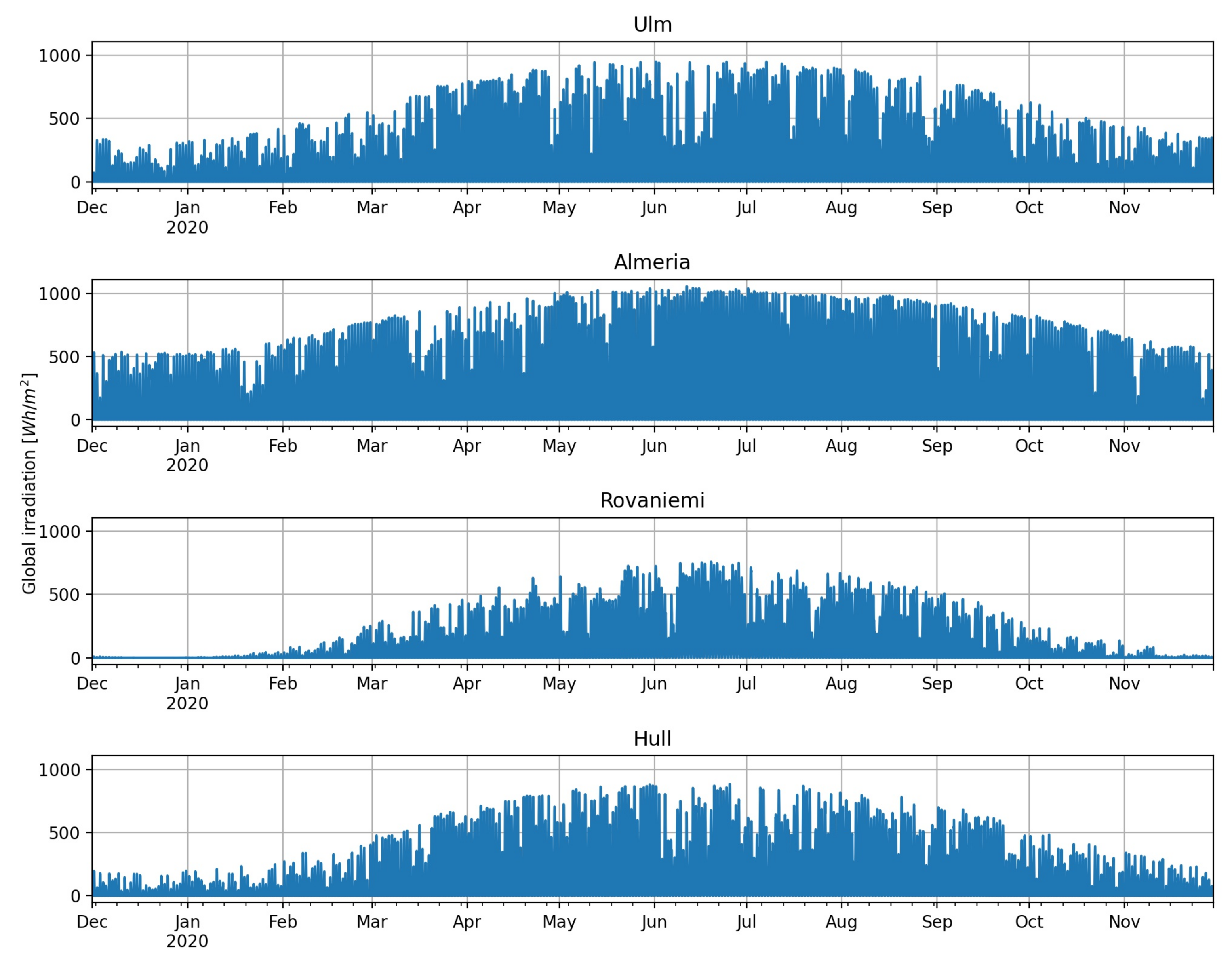
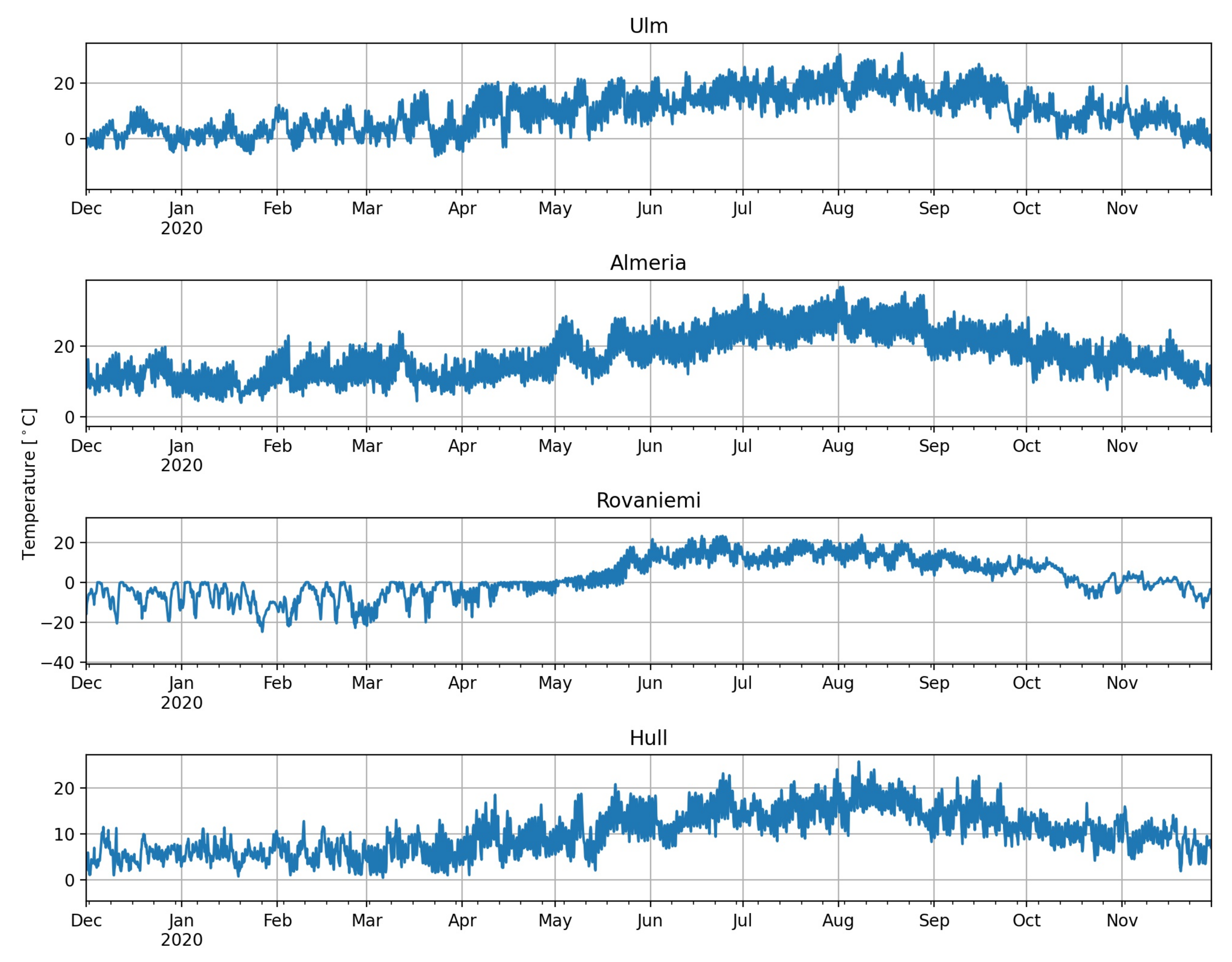
In total we have six univariate time series at four locations, and showing all data sets would simply be too much. Instead, to highlight some important features, we limit the visualisation to one year of solar irradiation and temperature data for all four locations, which are displayed in Figure 2 and 
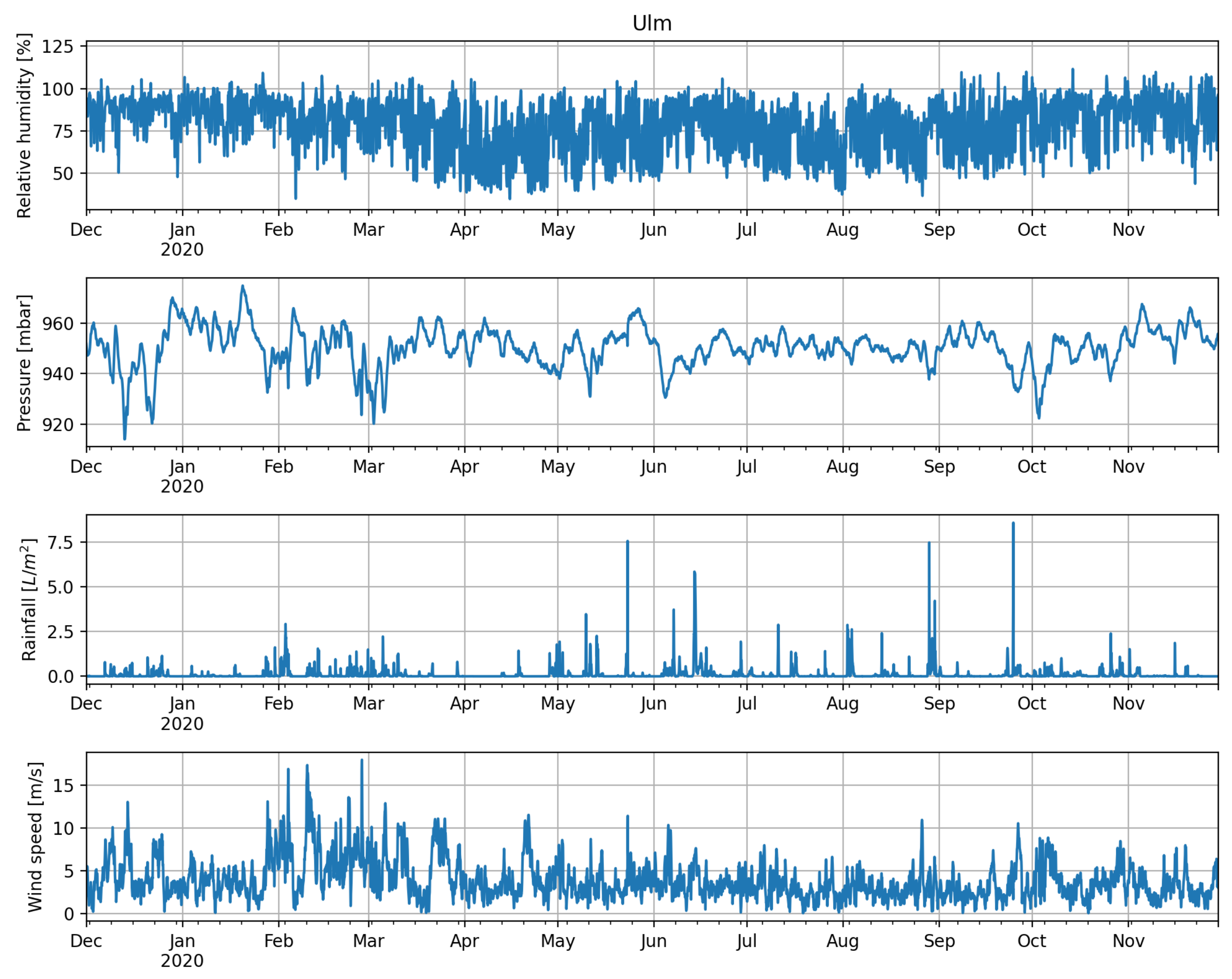
Figure 3. For Ulm, as the most central location, we also plot one year of humidity, wind speed, pressure, and rainfall in Figure 4. A visualization of the input data for all other locations can be found under the aforementioned GitHub link. Both global irradiation and temperature data show the expected annual swing, whereby the volatility of the irradiation data is considerably larger. Besides, irradiation levels are on average higher in Almeria and Ulm than in Rovaniemi and Hull. The same holds true for the temperature, where we see significantly larger oscillation during winter than during summer in Rovaniemi. Considering the other input factors for Ulm in Figure 4, one might assume that the distribution of humidity is slightly asymmetric, whereas pressure shows comparably less variation. Wind speed is—compared to the other data sets—a fairly noisy time series with time-varying volatility. Rainfall shows hardly any annual pattern but some extreme solitary spikes. To sum up our observations: for each location we have six quite diverse data sets, whereby often we have to deal with some kind of instationarity, e.g., potentially time-varying seasonality, spikes, or time-dependent volatility. A forecasting model needs to consider all these aspects.

4.2. Model Architecture and Calibration

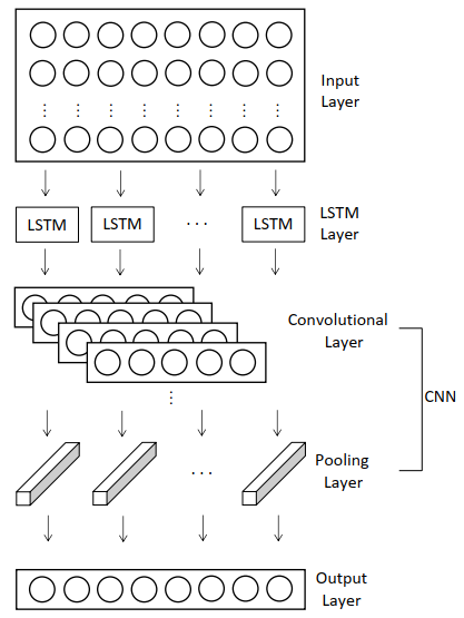
The objective of this article is to generate hourly solar irradiation forecasts. Models are chosen and calibrated to minimize the average expected error. In large part we based our architecture on the proposed models from related articles with similar objectives [7,33,48]. Hence, we make use of their results, whereby we have to adapt the models to our setup. For example, Wang et al. [7] used more LSTM units and two CNN layers (convolutional and max pooling layers) in their hybrid model. We fit the models to our data sets by trial and error where different setups are tested and the best one is chosen. Thereby one has to consider that including too many LSTM units may cause the network to adapt too much to a specific data set, which is called overfitting. Hence, in order to yield a trained NN that is able to handle new data points (which is the case in forecasting), we limit the number of LSTM units. For the convolutional part of the models we opted for a shallow architecture as we use 1D convolution. Based on that we evaluated the performance of different architectures and parameter combinations on the test set of a whole year and selected the best one. For example, we tested the effect of adding more convolutional layers, different amounts of kernels, different kernel sizes, and so on. The integration of max pooling layers was also investigated. Apart from that, layer order (whether LSTM or CNN first) does influence the NN setup. Thereby we found out that more convolutional kernels are needed if the data is convoluted first. The architecture and training parameters of all models considered here can be found in Appendix A.
As input for the NNs, we use 24 time steps to predict the next 24 h. To train the NNs we first split the data into a training, validation, and test set. The training and validation sets are handed to the NNs, whereas the testing set is kept for evaluating the model’s performance against real data (out of sample testing). In order to see how the NN performs over the course of a whole year, the test set contains data for one year, which means 8760 h. For the remaining data set we follow Wang et al. [7] and split it into 80 % training data and 20 % validation data, which is a common ratio in practice. Kreuzer et al. [6], for example, use the same ratio. To be on the safe side we also tested other ratios like 90 % vs. 10 % but could not find significant differences. Apart from that, the time index is transformed with sine and cosine to catch the periodicity. This is done by fitting the day/year data to a sine/cosine oscillation by dividing the timestamp by the day/year. Then sine/cosine is applied and we obtain four variables, namely day sine, day cosine, year sine, and year cosine.
Moreover, for facilitating the NN data processing, we normalize all data by scaling each input factor to values between 0 and 1 using a MinMax scaler [54]: Given a data sample X 1 , , X T the scaled value X t s c a l e d is calculated as follows:
X t s c a l e d = X t X m i n X m a x X m i n ,
where X m a x = max t = 1 , , T X t and X m i n = min t = 1 , , T X t .

4.3. Goodness of Fit Measures

We compute the root mean square error and the mean absolute error to evaluate the performance of the different forecasting models. The measures are calculated separately for each horizon k. Let X ^ t ( k ) be k-step forecast of X t . Then, the RMSE for the forecasting horizon k is defined as:
RMSE ( k ) = 1 T t = 1 T ( X t ( k ) X ^ t ( k ) ) 2 .
where T is the sample size. In our case the size of the test set is 8760, for example. The MAE is defined analogously:
MAE ( k ) = 1 T t = 1 T | X t ( k ) X ^ t ( k ) | .
In order to compare the average error over all tested forecasting horizons, we eventually compute the average for both RMSE and MAE:
RMSE total = 1 K k = 1 K RMSE ( k ) ; MAE total = 1 K k = 1 K MAE ( k ) ,
where K is the maximum number of predicted time steps, so here K = 24 . The unit of these measures is Wh/m2, as we forecast global irradiation values. Furthermore, to also compare results from different locations, a measure that adjusts for the local solar irradiation amount is needed. As level adjustment, the seasonal naive forecast at each location is used. We divide the models’ MAE by the MAE of the seasonal naive forecast (SN) and call it relative MAE (RMAE).
RMSE = MAE model MAE SN
Note that night hours are removed before computing the above described error measures as those hours naturally reduce all models’ errors without offering more insight.

4.4. Results and Performance Evaluation

Each model was trained for each location according to the process described in Section 4.2. The trained NNs were then tested on hourly climate data from 1 December 2019 to 30 November 2020. In the context of a rolling time window we fed the realized input values (Section 4.1) of the previous 24 h to the NNs in order to obtain irradiation forecasts for the upcoming 24 h. Results were compared to the true measured irradiation to obtain error values for each of the 24 forecasted hours. Eventually, having shifted the time window through the year, we obtained a vector of errors for each combination of forecasting horizon, model, and location. Eventually, these error vectors were evaluated and aggregated using the GoF measures described in Section 4.3.
Given all results we can state that merging a CNN with an LSTM model does indeed improve the forecasting performance. However, it is not the precision but the model’s robustness regarding climate conditions that matters.
Before presenting the results for all tested locations we need to verify if and how adding the MSI to the input data set makes sense. Regarding test results we only discuss Ulm here, as the results for the other locations are very similar: adding the MSI to the input only slightly reduces forecasting errors as shown in Table 3. Alternatively, as the MSI can be calculated for any location and any time over the year, we might add future MSI values (up to 24 h in advance) to the input set as well. Results from Table 3 show that errors are not significantly smaller either. The performance even decreases for some models (see convLSTM). Hence, we only use the factors from Table 2 and the MSI as input for all models.
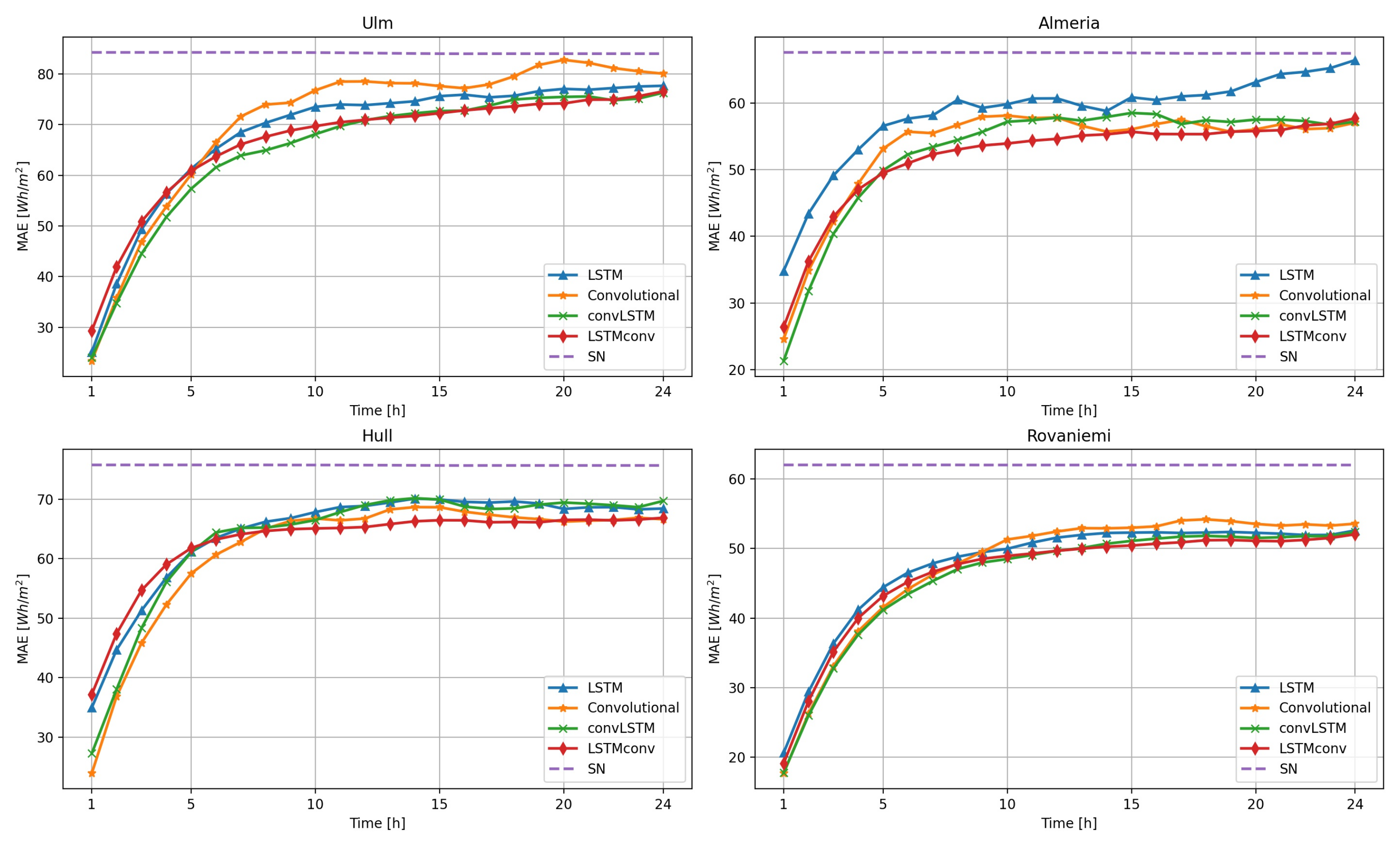
Having settled the issue if and how to include the MSI, we compute 24 h ahead forecasts for all locations and different neural network models, namely the LSTM network, the CNN, and both hybrid convLSTM and LSTMconv. The forecasts are evaluated using the GoF measures from Section 4.3. Results for all four cities are displayed in Figure 5, where the MAE for each individual hour of the 24 h ahead forecast is shown. The errors are thereby calculated based on the above described test set, i.e., for 8760 h from 1 December 2019 to 30 November 2020. From the graphic representation we can draw some major conclusions: First and foremost, except for the seasonal naive forecast, MAE values of the different NN models differ only slightly. In the first few hours the convolutional and convLSTM network perform the best. Later on the CNN is outperformed and overall the LSTMconv model seems to perform the best. The simple LSTM model has the worst performance, which is still close to the others. By comparing the cities we notice that here the main difference is the the error level. In Rovaniemi, where we have big seasonal differences (no solar irradiation in winter, all day irradiation in summer), the error is the lowest (MAE is roughly around 50 Wh/mM2), whereas in Ulm with no specific seasonal pattern the network forecasts result in the largest errors (MAE is roughly around 75 Wh/m2).
The aggregated results for all models and exemplary for the cities Ulm and Almeria are shown in Table 4, whereby the best results are highlighted in bold letters. Values for Hull and Rovaniemi are given in Appendix A. Thereby, results from Table 4 just confirm the graphical observations. In general, combining an CNN with an LSTM model increases forecasting precision.
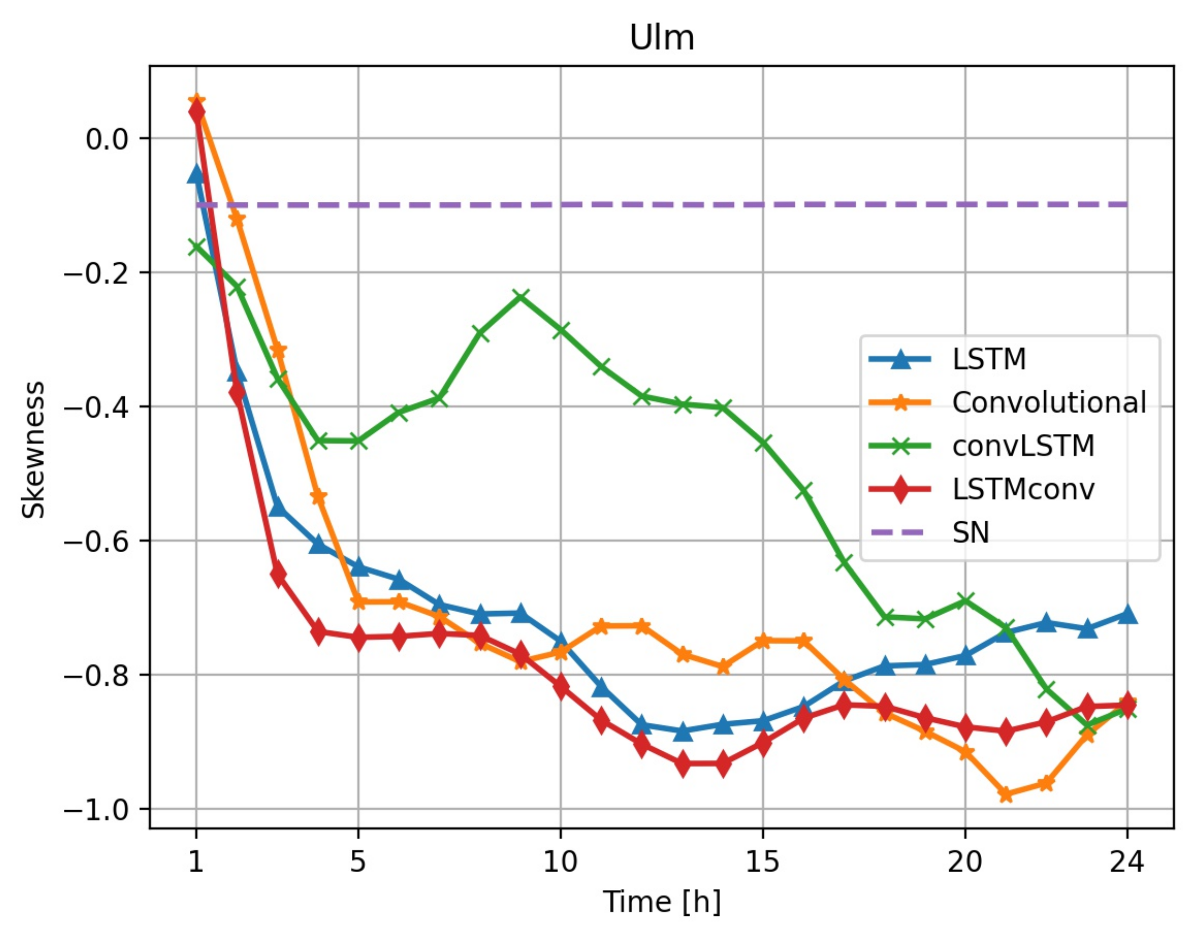
For more insight into the models’ performance we also consider some distributional properties. Thereby we see that, except for the convolutional model, all models are more or less unbiased. The bias of the naive forecast is closest to zero, whereas the convolutional model’s bias is positive. Hence, as the error is computed as true irradiation minus forecasted irradiation ( X t ( k ) X ^ t ( k ) ), the convolutional model tends to underestimate irradiation levels. Besides, at all locations and for all considered forecasting horizons we find that model errors are negatively skewed. In 
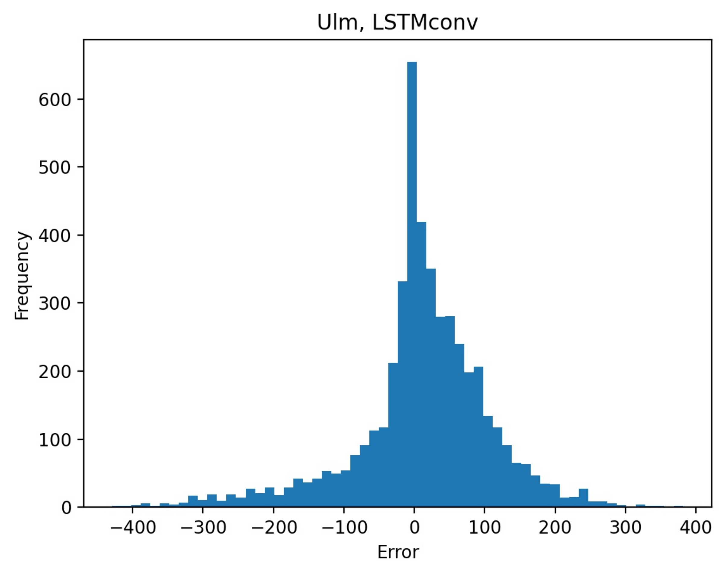
Figure 6, where this fact is exemplarily shown for Ulm, we see a quite uniform behavior except for the convLSTM, which is still skewed. Negative skewness means that, when overestimating irradiation, the risk of missing the real value significantly is larger than when underestimating irradiation. The skewness is clearly visible in Figure 7 where the histogram of the six hour-ahead forecast for the LSTMconv model for Ulm is displayed.
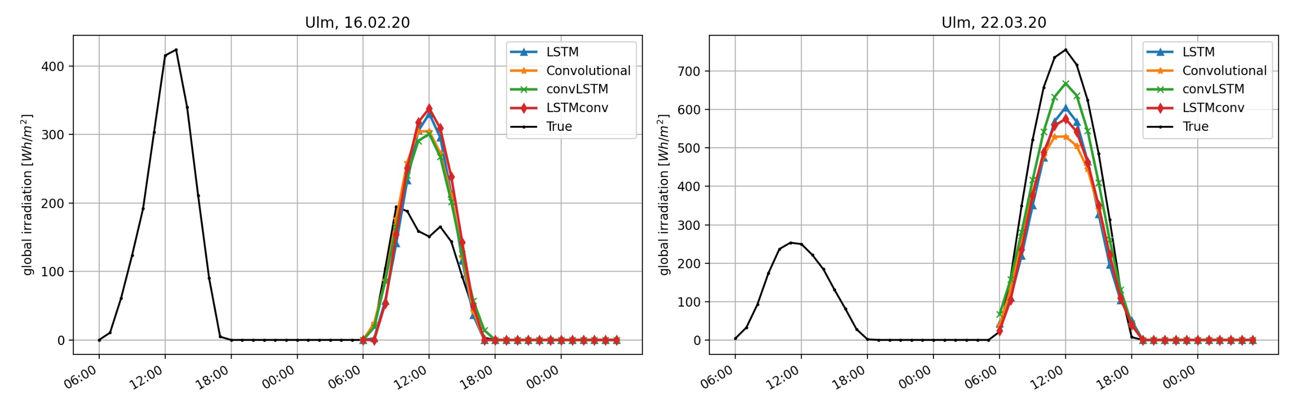
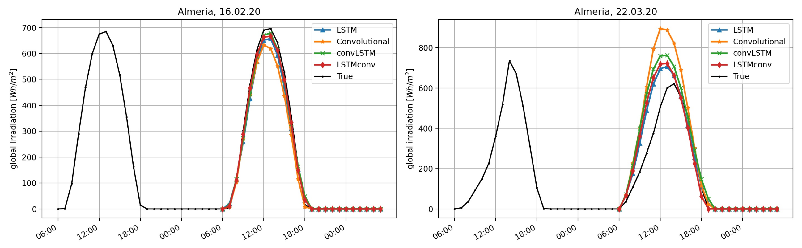
To visualize the models’ performance for two specific situations, we plot the forecasting results of each model in Figure 8, Figure 9, Figure 10 and 
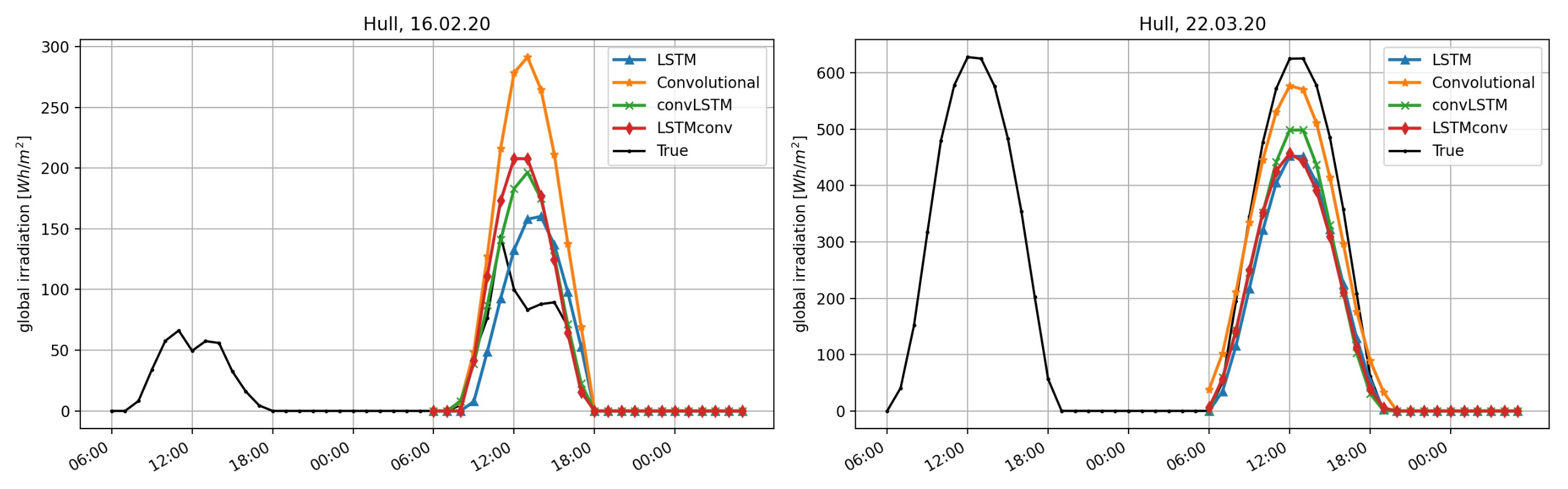
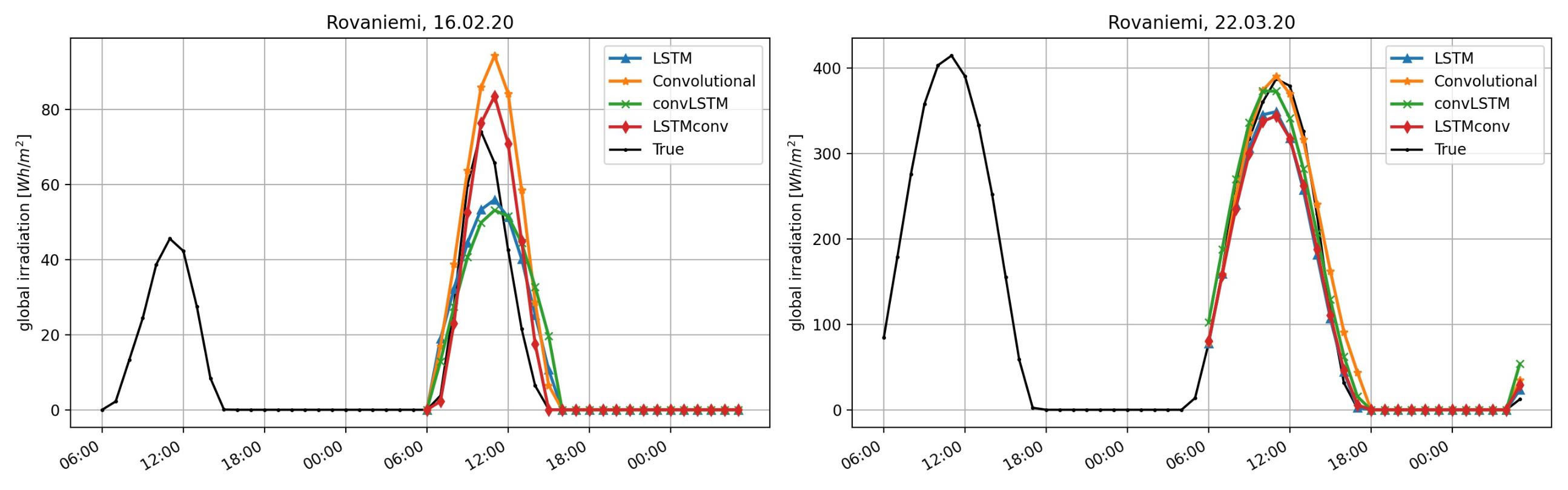
Figure 11: A 24 h ahead forecast was computed for two days at 6 a.m. The right graphic shows the irradiation forecasts for 22 March 2020. For Ulm, for example, we see that even though the irradiation on the previous day (input data) is on a low level, all NNs are able to predict more or less the correct irradiation level. Nevertheless, the forecast is lower than the actual irradiation. On 16 February 2020 (left plot) there is a irradiation drop in Ulm around noon, which was not incorporated by any NN. The same can be seen for Hull in Figure 10 on the left side. Interestingly, in Figure 10 and Figure 11, we see a rather diverse performance of the NN algorithms for 16 February 2020. In both cases the CNN was clearly overstimating sunshine levels. In Rovaniemi, the LSTMconv model produced the closest estimate, wherease LSTM and convLSTM signifcantly underestimated sunshine levels. The day in March seemed to be a fairly sunny day with no surprises and all models performed quite well for all locations except for Almeria, where no model was able to capture the seemingly asymmetric pattern with less sunshine in the morning hours.
To compare all locations with each other we eventually focus on the best model, namely the LSTMconv network. First we identify the mean solar irradiation for each location, whereby we only consider hours with positive values. Each MAE is then divided by this aggregated number and results are displayed in Table 5, which confirms the assumption that the NNs perform better in sunny regions (e.g., Almeria) than in regions with unstable weather like Ulm or Hull. Without the adjustment, Rovaniemi has the lowest MAE, which is reasonable as during winter there is no sun and during summer there is comparably lesser sun than, say, in Almeria. Hence, it is reasonable to expect absolute differences to be smaller. Note that we could have alternatively computed the mean absolute percentage error, which divides the absolute error by the current irradiation level. However, as in the morning and in the evening irradiation levels are very small, this alternative error measure often produces extremely high error levels which significantly skews the total GoF measure. This is why we consider the adjusted MAE to be a better measure for comparison.
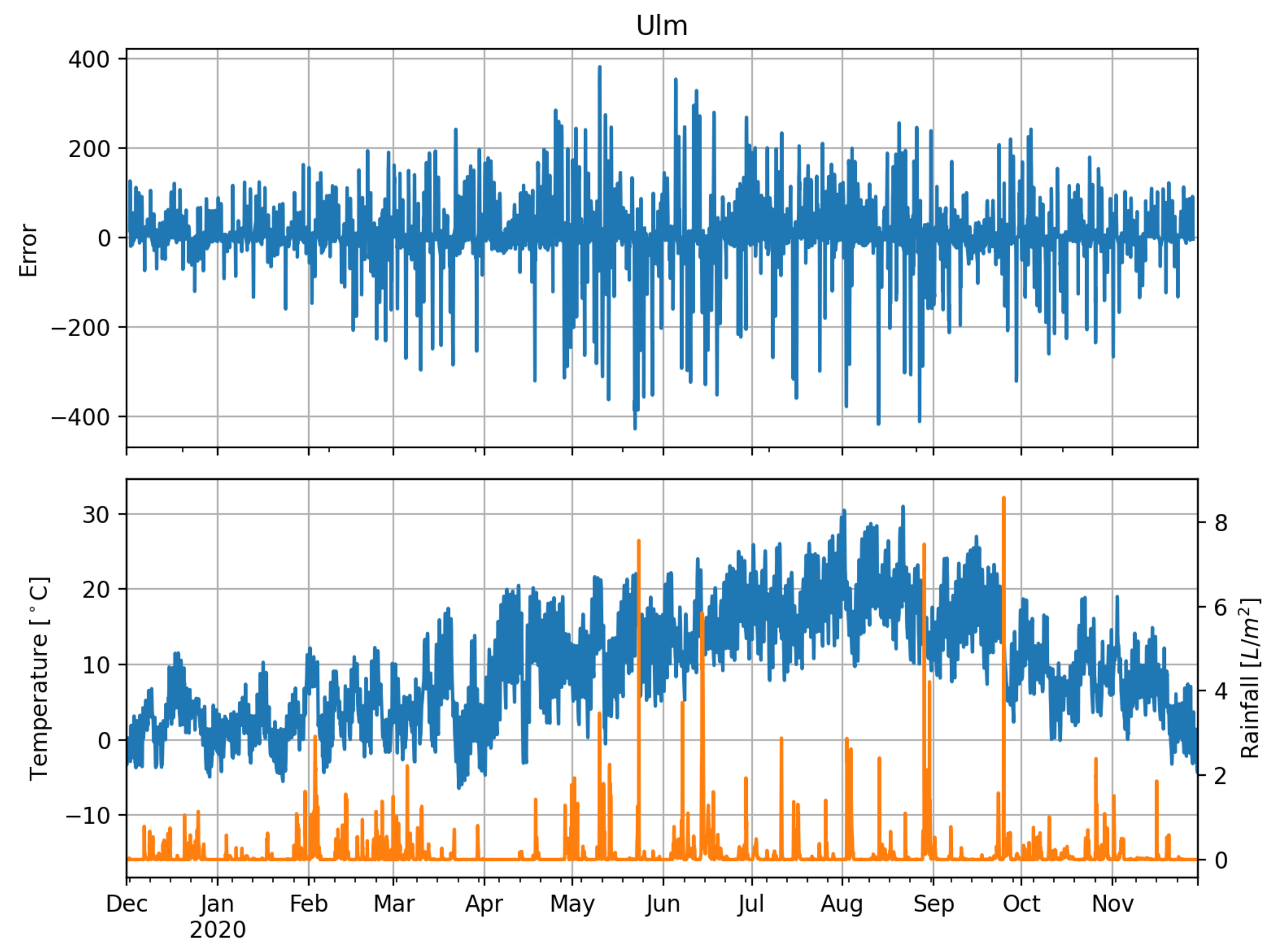
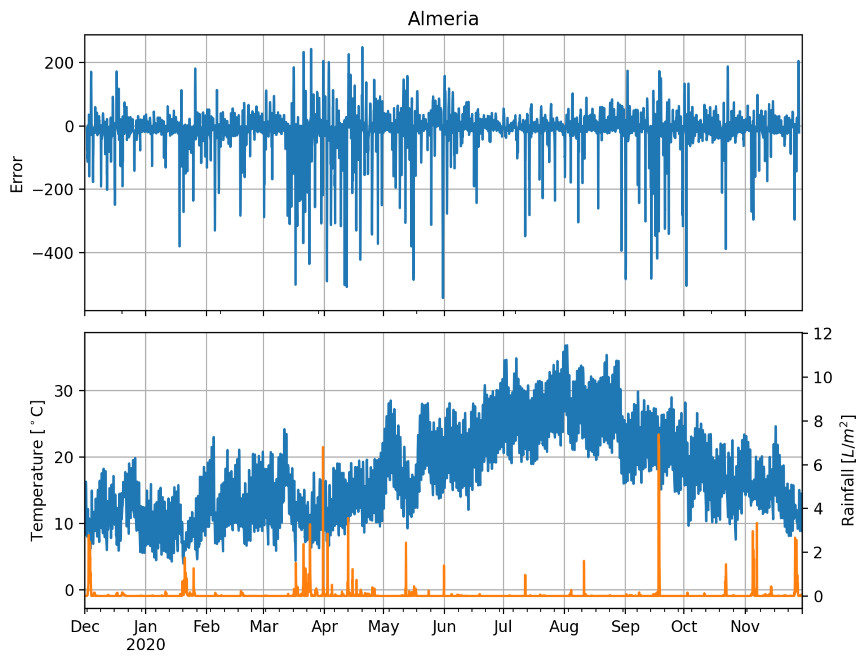
Having identified the LSTMconv as a model that performs good under all conditions, we eventually analyze the errors in the time domain, where we use Figure 12, Figure 13, Figure 14 and 
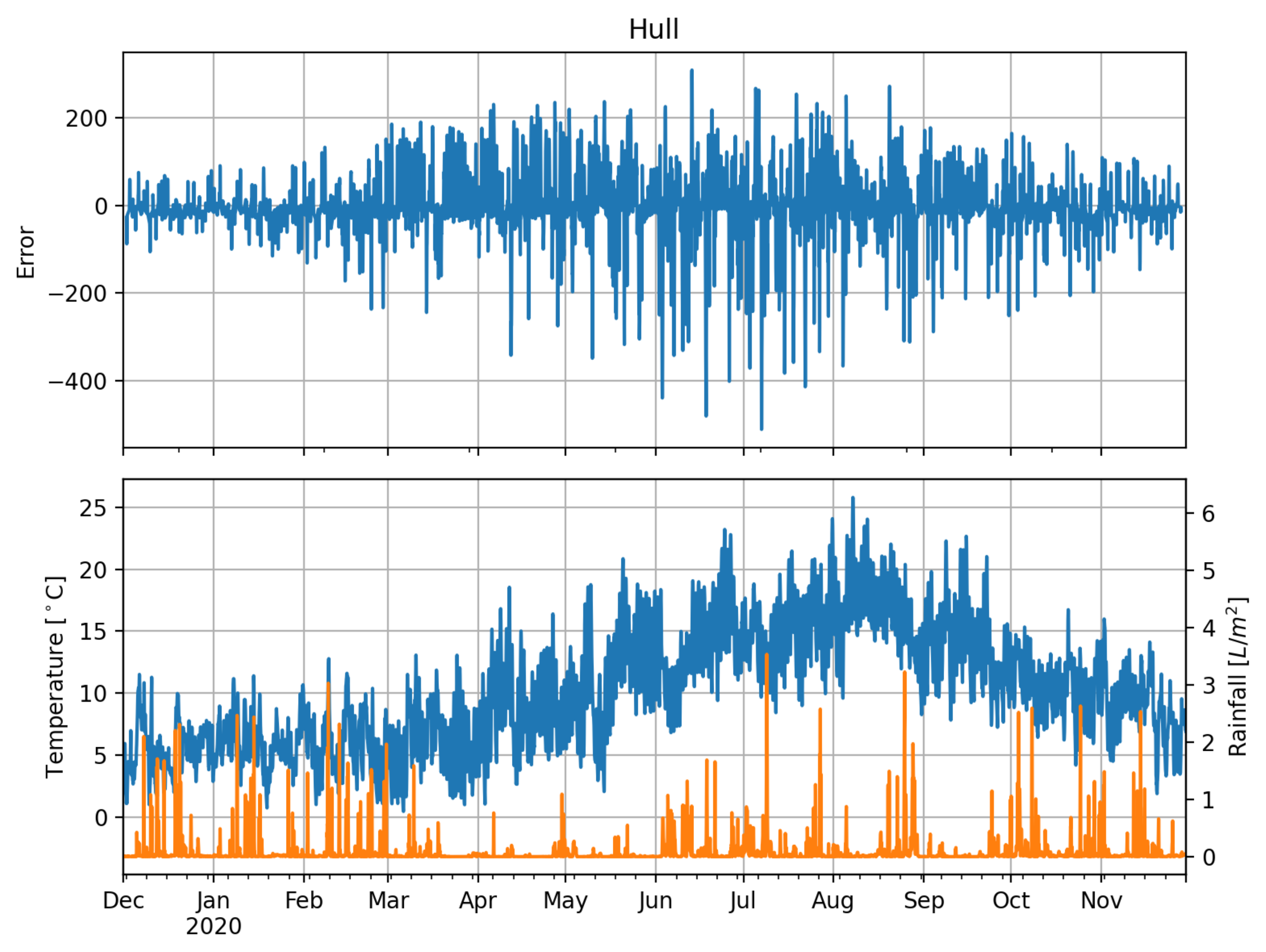
Figure 15 as graphical means to extract information about the model’s performance. Note that we limit our comparison to this model as it proves to be sufficient. The same conclusions can be drawn for the other NN models. The errors in Ulm show a distinct annual pattern with smaller absolute values in winter than in summer—which is not the case for Almeria. In fact, here it is the other way round. During July/August errors are comparably small whereas during April and May, where both temperature and precipitation indicate comparably cold and wet weather, error variation is larger than during the other months. Given the plot, Almeria errors are also skewed to the left but more distinctly than Ulm errors. Errors of Hull (
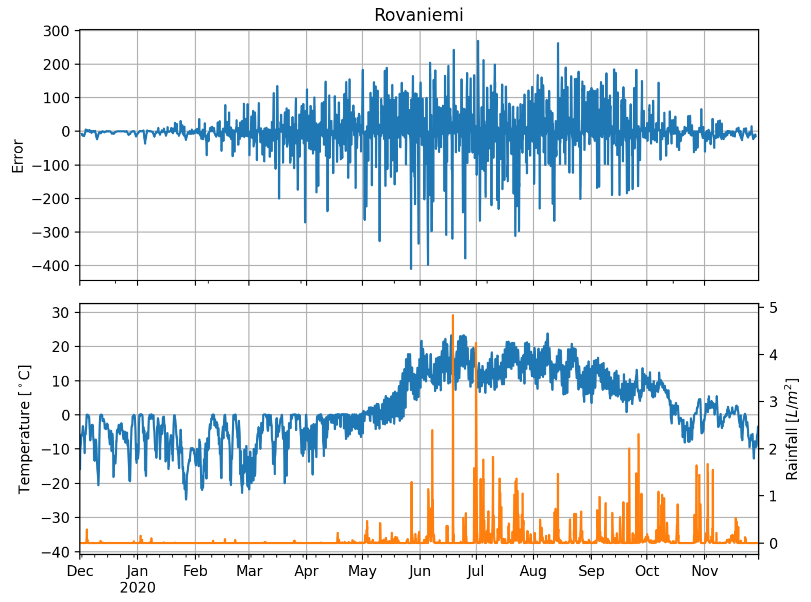
Figure 14) are low during winter season, which goes along with less sunshine, low temperatures, and comparatively a lot of rain. We see a distinct annual pattern in the forecasting error, which only partly coincides with the annual temperature swing. Eventually, Rovaniemi errors show the expected pattern: almost no errors during winter when it is dark anyway. Forecasting errors do not significantly coincide with the annual temperature swing or rainfall. As for Hull, errors seem to be mainly dependent on the annual swing of irradiation (compare Figure 2).
To sum up our results: the LSTMconv neural network performs best in our case study across all tested locations. However, the advantage is small—especially when considering that the training process of the neural networks appeared to be not deterministic. This means that the results vary—albeit very little—when training the same network multiple times. Furthermore, the problem of the non-deterministic training process makes fine tuning of the neural networks quite hard. So, the LSTM seems like a good alternative; however, its performance for sunny Almeria is comparably worse. The CNN, again, has problems with the continental climate of Ulm but would be a feasible alternative for the other locations. Hence, the LSTMconv network is the best model not because it produces the best results but because it appears to be a rather versatile approach producing fairly good results in all tested climate conditions.
In terms of computational time, all networks are feasible for practical application as the training, which has to be done once a day or once a week, requires less then 30 min on a regular laptop.

5. Conclusions

Using neural networks for forecasting purposes has become very fashionable lately. This is proven by the wide range of literature about this topic. The motivation simply is that NNs show a comparably good performance and authors have tried to improve on these levels by combining different types of NNs. In this article we analyze the suitability for solar irradiation forecasting by comparing the performance of different NN models, namely an LSTM, a CNN, and two hybrid versions. We consider short-term forecasts up to 24 h ahead and test the models on four different locations in Europe to check the local climate’s influence on the overall behavior. It shows that the hybrid versions, i.e., the combination of a CNN and an LSTM model, outperform the other models, but the advantage is not significant—given our data sets and the tested climate conditions. Except for Almeria, the sunniest location, a comparably simple LSTM performs very similar to a more complex combination of CNN and LSTM model. However, the additional complexity does pay off, because even if the forecasting error is not considerable smaller compared to the other tested NNs, the hybrid models are more robust against changing climate conditions. The LSTM model has problems in sunny regions, the CNN for Ulm, i.e., a continental climate. The hybrid methods produce good forecasts in all scenarios. Eventually, as we use data that are easily available online and because the source code of this article is publicly available on GitHub, the NN-based methods presented in this study can be easily transferred to any other location worldwide. This is beneficial, as there is still some research to be done. First, one might check the models’ performance at more locations across the planet. Longer data sets might increase the reliability of the results. However, as we work with hourly values, one year should already guarantee significance of the results. Second, when analyzing more years in the test data set one could study seasonal differences.

Author Contributions

Conceptualization, S.L. and S.S.; methodology, S.L. and S.S.; software, S.L.; validation, S.L. and S.S.; formal analysis, S.L. and S.S.; investigation, S.L., J.-S.U. and Y.H.; resources, S.L.; data curation, Y.H.; writing—original draft preparation, S.L. and S.S.; writing—review and editing, S.L., J.-S.U., Y.H. and S.S.; visualization, S.L.; supervision, S.S.; project administration, S.S. All authors have read and agreed to the published version of the manuscript.

Funding

This work was supported by the “Human Resources Program in Energy Technology” of the Korea Institute of Energy Technology Evaluation and Planning (KETEP), granted financial resource from the Ministry of Trade, Industry & Energy, Republic of Korea. (No. 20194010000040).

Data Availability Statement

Data can be downloaded free of charge for research purposes via www.soda-pro.com (accessed on 21 May 2021).

Acknowledgments

The authors would like to thank David Kreuzer for his valuable comments and tips regarding Python coding.

Conflicts of Interest

The authors declare no conflict of interest.

Abbreviations

The following abbreviations are used in this manuscript:
ANNArtificial neural network
CNNConvolutional neural network
LSTMLong-short term memory (neural network)
MAEMean absolute error
MSIMaximum solar irradiation
NNNeural network
RMAERelative mean absolute error
RMSERoot mean square error
RNNRecurrent neural networks
SARIMASeasonal autoregressive integrated moving average (model)
SNSeasonal naive

Appendix A

Table A1. Performance results of the different NN models for the cites Hull and Rovaniemi.
ModelHullRovaniemi
RMSEMAERMAERMSEMAERMAE
LSTM91.5064.3985.06%72.3347.6576.83%
CNN92.8261.5981.36%74.2147.5676.68%
convLSTM91.2363.5483.94%71.2546.0074.16%
LSTMconv91.0962.8783.05%71.5946.3874.78%
Table A2. Architecture of the LSTM network.
CategoryParameterValueDescription
LSTM layerunits32number of LSTM cells
dense layerunits24number of hours to predict
traininglossMSEmean square error
trainingoptimizerADAM optimizer
traininglearning rate0.0001learning rate of optimizer
Table A3. Architecture of the convolutional network.
CategoryParameterValueDescription
Conv1D layerfilters64number of filters
Conv1D layerkernel size3size of a filter
MaxPool1D layerpool size2size of MaxPool kernel
Conv1D layerfilters64number of filters
Conv1D layerkernel size2size of a filter
MaxPool1D layerpool size2size of MaxPool kernel
flatten layer
dense layerunits24amount of hours to predict
traininglossMSEmean square error
trainingoptimizerADAM optimizer
traininglearning rate0.001learning rate of optimizer
Table A4. Architecture of the convolutional LSTM network.
CategoryParameterValueDescription
Conv1D layerfilters256number of filters
Conv1D layerkernel size3size of a filter
Conv1D layerfilters256number of filters
Conv1D layerkernel size2size of a filter
MaxPool1D layerpool size2size of MaxPool kernel
LSTM layerunits32number of LSTM cells
dense layerunits24number of hours to predict
traininglossMSEmean square error
trainingoptimizerADAM optimizer
traininglearning rate0.0001learning rate of optimizer
Table A5. Architecture of the LSTM convolutional network.
CategoryParameterValueDescription
LSTM layerunits32number of LSTM cells
Conv1D layerfilters256number of filters
Conv1D layerkernel size3size of a filter
MaxPool1D layerpool size2size of MaxPool kernel
flatten layer
dense layerunits24number of hours to predict
traininglossMSEmean square error
trainingoptimizerADAM optimizer
traininglearning rate0.00001learning rate of optimizer

References

  1. Michalsky, J.J. The Astronomical Almanac’s algorithm for approximate solar position (1950–2050). Sol. Energy 1988, 40, 227–235. [Google Scholar] [CrossRef]
  2. Bird, R.E.; Hulstrom, R.L. A Simplified Clear Sky Model for Direct and Diffuse Insolation on Horizontal Surfaces. NREL Tech. Rep.; 1981. Available online: https://www.nrel.gov/docs/legosti/old/761.pdf (accessed on 21 May 2021).
  3. Lorenz, E.; Hurka, J.; Heinemann, D.; Beyer, H. Irradiance forecasting for the power prediction of grid-connected photovoltaic systems. IEEE J. Sel. Top. Appl. Earth Obs. Remote Sens. 2009, 2, 2–10. [Google Scholar] [CrossRef]
  4. Müller, S.; Remund, J. Advances in Radiation Forecast Based on Regional Weather Models MM5 and WRF. In Proceedings of the 25th European Photovoltaic Solar Energy Conference, Valencia, Spain, 6–10 September 2010; pp. 4629–4632. [Google Scholar]
  5. Hill, T.; O’Connor, M.; Remus, W. Neural Network Models for Time Series Forecasts. Manag. Sci. 1996, 47, 1082–1092. [Google Scholar] [CrossRef]
  6. Kreuzer, D.; Munz, M.; Schlüter, S. Short-term temperature forecasts using a convolutional neural network — An application to different weather stations in Germany. Mach. Learn. Appl. 2020, 2, 100007. [Google Scholar] [CrossRef]
  7. Wang, K.; Qi, X.; Liu, H. Photovoltaic power forecasting based LSTM-Convolutional Network. Energy 2019, 189, 116225. [Google Scholar] [CrossRef]
  8. Bakker, K.; Whan, K.; Knap, W.; Schmeits, M. Comparison of statistical post-processing methods for probabilistic NWP forecasts of solar radiation. Sol. Energy 2019, 191, 138–150. [Google Scholar] [CrossRef]
  9. Yeom, J.-M.; Deo, R.-C.; Adamwoski, J.F.; Chae, T.; Kim, D.-S.; Han, K.-S.; Kim, D.-Y. Exploring solar and wind energy resources in North Korea with COMS MI geostationary satellite data coupled with numerical weather prediction reanalysis variables. Renew. Sustain. Energy Rev. 2020, 119, 109570. [Google Scholar] [CrossRef]
  10. Murata, A.; Ohtake, H.; Oozeki, T. Modeling of uncertainty of solar irradiance forecasts on numerical weather predictions with the estimation of multiple confidence intervals. Renew. Energy 2018, 117, 193–201. [Google Scholar] [CrossRef]
  11. Perez, R.; Kivalov, S.; Schlemmer, J.; Hemker, K.; Zelenka, A. Improving the Performance of Satellite-to-Irradiance Models using the Satellite’s Infrared Sensors. In Proceedings of the 39th ASES National Solar Conference 2010, Phoenix, AZ, USA, 17–22 May 2010. [Google Scholar]
  12. Pelland, S.; Galanis, G.; Kallos, G. Solar and photovoltaic forecasting through post-processing of the Global Environmental Multiscale numerical weather prediction model. Prog. Photovolt. Res. Appl. 2013, 21, 284–296. [Google Scholar] [CrossRef]
  13. Ernst, B.; Reyer, F.; Vanzetta, J. Wind Power and Photovoltaic Prediction Tools for Balancing and Grid Operation. In Proceedings of the CIGRE/IEEE PES Joint Symposium Integration of Wide-Scale Renewable Resources into the Power Delivery System, Calgary, AB, Canada, 29–31 July 2009. [Google Scholar]
  14. Chaouachi, A.; Kamel, R.; Nagasaka, K. Neural network ensemble-based solar power generation short-term forecasting. J. Adv. Comput. Intell. Intell. Inform. 2010, 14, 69–75. [Google Scholar] [CrossRef] [Green Version]
  15. Möller, A.; Groß, J. Probabilistic temperature forecasting based on an ensemble autoregressive modification. Q. J. R. Meteorol. Soc. 2016, 142, 1385–1394. [Google Scholar] [CrossRef] [Green Version]
  16. Kann, A.; Haiden, T.; Wittmann, C. Combining 2-m temperature nowcasting and short range ensemble forecasting. Nonlinear Process. Geophys. 2011, 18, 903–910. [Google Scholar] [CrossRef] [Green Version]
  17. Hassani, H.; Silva, E.S.; Gupta, R.; Das, S. Predicting global temperature anomaly: A definitive investigation using an ensemble of twelve competing forecasting models. Phys. A Stat. Mech. Appl. 2018, 509, 121–139. [Google Scholar] [CrossRef]
  18. McNeil, A.J.; Frey, R.; Embrechts, P. Quantitative Risk Management: Concepts, Techniques and Tools; Revised ed.; Princeton University Press: Princeton, NJ, USA, 2015; pp. 125–157. [Google Scholar]
  19. Lin, G.-Q.; Li, L.-L.; Tseng, M.L.; Liu, H.-M.; Yuan, D.-D.; Tan, R.-R. An improved moth-flame optimization algorithm for support vector machine prediction of photovoltaic power generation. J. Clean. Prod. 2020, 253, 119966. [Google Scholar] [CrossRef]
  20. VanDeventer, W.; Jamei, E.; Thirunavukkarasu, G.S.; Seyedmahmoudian, M.; Soon, T.K.; Horan, B.; Mekhilef, S.; Stojcevski, A. Short-term PV power forecasting using hybrid GASVM technique. Renew. Energy 2019, 140, 367–379. [Google Scholar] [CrossRef]
  21. Zendehboudi, A.; Baseer, M.; Saidur, R. Application of support vector machine models for forecasting solar and wind energy resources: A review. J. Clean. Prod. 2018, 199, 272–285. [Google Scholar] [CrossRef]
  22. Abdel-Nasser, M.; Mahmoud, K. Accurate photovoltaic power forecasting models using deep lstm-rnn. Neural Comput. Appl. 2019, 31, 2727–2740. [Google Scholar] [CrossRef]
  23. Lee, D.; Kim, K. Recurrent Neural Network-Based Hourly Prediction of Photovoltaic Power Output Using Meteorological Information. Energies 2019, 12, 215. [Google Scholar] [CrossRef] [Green Version]
  24. Benali, L.; Notton, G.; Fouilloy, A.; Voyant, C.; Dizene, R. Solar radiation forecasting using artificial neural network and random forest methods: Application to normal beam, horizontal diffuse and global components. Renew. Energy 2019, 132, 871–884. [Google Scholar] [CrossRef]
  25. Ozoegwu, C.G. Artificial neural network forecast of monthly mean daily global solar radiation of selected locations based on time series and month number. J. Clean. Prod. 2019, 216, 1–13. [Google Scholar] [CrossRef]
  26. Pereira, S.; Canhoto, P.; Salgado, R.; Costa, M.J. Development of an ANN based corrective algorithm of the operational ECMWF global horizontal irradiation forecasts. Sol. Energy 2019, 185, 387–405. [Google Scholar] [CrossRef]
  27. Gensler, A.; Henze, J.; Sick, B.; Raabe, N. Deep Learning for Solar Power Forecasting-an Approach Using AutoEncoder and LSTM Neural Networks. In Proceedings of the 2016 IEEE International Conference on Systems, Man and Cybernetics (SMC), Budapest, Hungary, 9–12 October 2016. [Google Scholar]
  28. Lima, M.A.F.; Carvalho, P.C.; Fernandes-Ramirez, L.M.; Braga, A.P. Improving solar forecasting using Deep Learning and Portfolio Theory. Energy 2020, 195, 117016. [Google Scholar] [CrossRef]
  29. Yang, D.; Xiong, T.; Xu, D.; Zhou, K.; Xu, Z.; Chen, M.; Park, J.H.; Grbic, S.; Tran, T.D.; Chin, S.P.; et al. Deep Image-to-Image Recurrent Network with Shape Basis Learning for Automatic Vertebra Labeling in Large-Scale 3D CT Volumes. In Proceedings of the International Conference on Medical Image Computing and Computer-Assisted Intervention, Quebec City, QC, Canada, 10–14 September 2017; pp. 498–506. [Google Scholar]
  30. Zhu, L.; Chen, H.; Ye, W. A Hybrid CNN–LSTM Network for the Classification of Human Activities Based on Micro-Doppler Radar. IEEE Access 2020, 8, 24713–24720. [Google Scholar] [CrossRef]
  31. Islam, M.Z.; Islam, M.M.; Ashraf, A. A combined deep CNN-LSTM network for the detection of novel coronavirus (COVID-19) using X-ray images. Inform. Med. Unlocked 2020, 20, 100412. [Google Scholar] [CrossRef] [PubMed]
  32. He, Z.; Zhou, J.; Dai, H.N.; Wang, H. Gold Price Forecast Based on LSTM-CNN Model. In Proceedings of the 2019 IEEE Intl Conf on Dependable, Autonomic and Secure Computing, Intl Conf on Pervasive Intelligence and Computing, Intl Conf on Cloud and Big Data Computing, Intl Conf on Cyber Science and Technology Congress (DASC/PiCom/CBDCom/CyberSciTech), Fukuoka, Japan, 5–8 August 2019; pp. 1046–1053. [Google Scholar]
  33. Livieris, I.E.; Pintelas, E.; Pintelas, P. A CNN-LSTM model for gold price time-series forecasting. Neural Comput. Appl. 2020, 32, 17351–17360. [Google Scholar] [CrossRef]
  34. Kim, T.; Kim, H.Y. Forecasting stock prices with a feature fusion LSTM-CNN model using different representations of the same data. PLoS ONE 2019, 14, e0212320. [Google Scholar] [CrossRef] [PubMed]
  35. Wu, J.M.T.; Li, Z.; Herencsar, N.; Vo, B.; Lin, J.C.-W. A graph-based CNN-LSTM stock price prediction algorithm with leading indicators. Multimed. Syst. 2021. [Google Scholar] [CrossRef]
  36. Li, T.; Hua, M.; Wu, X. A Hybrid CNN-LSTM Model for Forecasting Particulate Matter. IEEE Access 2020, 8, 26933–26940. [Google Scholar] [CrossRef]
  37. Baek, S.-S.; Pyo, J.; Chun, J.A. Prediction of Water Level and Water Quality Using a CNN-LSTM Combined Deep Learning Approach. Water 2020, 12, 3399. [Google Scholar] [CrossRef]
  38. Cao, K.; Kim, H.; Hwang, C.; Jung, H. CNN-LSTM Coupled Model for Prediction of Waterworks Operation Data. J. Inf. Process. Syst. 2018, 14, 1508–1520. [Google Scholar]
  39. Zou, J.; Han, Y.; So, S.-S. Overview over artificial networks. In Artificial Neural Networks Methods and Applications; Livingston, D.J., Ed.; Humana Press: Totowa, NJ, USA, 2009; pp. 12–23. [Google Scholar]
  40. Aggarwal, C.C. Neural Networks and Deep Learning, 1st ed.; Springer International Publishing: Cham, Switzerland, 2018. [Google Scholar]
  41. LeCun, Y.; Bottou, L.; Bengio, Y.; Haffner, P. Gradient-based learning applied to document recognition. Proc. IEEE 1998, 86, 2278–2324. [Google Scholar] [CrossRef] [Green Version]
  42. Hochreiter, S.; Schmidhuber, J. Long short-term memory. Neural Comput. 1997, 9, 1735–1780. [Google Scholar] [CrossRef]
  43. Karim, F.; Majumdar, S.; Darabi, H.; Chen, S. LSTM Fully Convolutional Networks for Time Series Classification. IEEE Access 2017, 6, 1662–1669. [Google Scholar] [CrossRef]
  44. Krizhevsky, A.; Sutskever, I.; Hinton, G.E. ImageNet Classification with Deep Convolutional Neural Networks. In Proceedings of the International Conference on Neural Information Processing Systems (NIPS2012), Lake Tahoe, NV, USA, 3–8 December 2012. [Google Scholar]
  45. Hinton, G.; Deng, L.; Yu, D.; Dahl, G.; Mohamed, A.; Jaitly, N.; Senior, A.; Vanhoucke, V.; Nguyen, P.; Sainath, T.N.; et al. Deep neural networks for acoustic modelling in speech recognition. IEEE Signal Process. Mag. 2012, 29, 82–97. [Google Scholar] [CrossRef]
  46. Jozefowicz, R.; Vinyals, O.; Schuster, M.; Shazeer, N.; Wu, Y. Exploring the Limits of Language Modeling. arXiv 2016, arXiv:1602.02410. Available online: https://arxiv.org/pdf/1602.02410.pdf (accessed on 21 May 2021).
  47. Borovykh, A.; Bohte, S.; Oosterlee, C.W. Conditional time series forecasting with convolutional neural networks. arXiv 2018, arXiv:1703.04691v5. Available online: https://arxiv.org/pdf/1703.04691v5.pdf (accessed on 21 May 2021).
  48. Koprinska, I.; Wu, D.; Wang, Z. Convolutional Neural Networks for Energy Time Series Forecasting. In Proceedings of the International Joint Conference on Neural Networks (IJCNN), Rio de Janeiro, Brazil, 8–13 July 2018. [Google Scholar]
  49. Understanding 1D and 3D Convolution Neural Network|Keras. Available online: https://towardsdatascience.com/understanding-1d-and-3d-convolution-neural-network-keras-9d8f76e29610 (accessed on 21 May 2021).
  50. Kiranyaz, S.; Avci, O.; Abdeljaber, O.; Ince, T.; Gabbouj, M.; Inman, D.J. 1D Convolutional Neural Networks and Applications—A Survey. 2019. Available online: https://arxiv.org/pdf/1905.03554.pdf (accessed on 21 May 2020).
  51. Lu, W.; Li, J.; Li, Y.; Sun, A.; Wang, J. A CNN-LSTM-Based Model to Forecast Stock Prices. Complexity 2020, 2020, 6622927. [Google Scholar] [CrossRef]
  52. Lamigueiro, O.P. solaR: Solar Radiation and Photovoltaic Systems with R. J. Stat. Softw. 2012, 50, 1–32. [Google Scholar] [CrossRef] [Green Version]
  53. Global Modeling and Assimilation Office (GMAO). MERRA-2 tavg1_2d_slv_Nx: 2d, 1-Hourly, Time-Averaged, Single-Level, Assimilation, Single-Level Diagnostics V5.12.4, Greenbelt, MD, USA, Goddard Earth Sciences Data and Information Services Center (GES DISC); 2015. Available online: https://disc.gsfc.nasa.gov/datasets/M2T1NXSLV_5.12.4/summary (accessed on 21 May 2021).
  54. Sola, J.; Sevilla, J. Importance of input data normalization for the application of neural networks to complex industrial problems. IEEE Trans. Nucl. Sci. 1997, 44, 1464–1468. [Google Scholar] [CrossRef]
Figure 1. Structure of LSTMconv model (based on [51]).
Energies 14 03030 g001
Figure 2. Global irradiation from 1 December 2019 to 30 November 2020.
Energies 14 03030 g002
Figure 3. Temperature from 1 December 2019 to 30 November 2020.
Energies 14 03030 g003
Figure 4. Other input factors from Ulm from 1 December 2019 to 30 November 2020.
Energies 14 03030 g004
Figure 5. MAE for various neural network models: LSTM, Convolutional, convolutional LSTM (convLSTM), and LSTM convolutional (LSTMconv). As reference the seasonal naive forecast (SN) is shown.
Energies 14 03030 g005
Figure 6. Skewness of the different NN models.
Energies 14 03030 g006
Figure 7. Histogram of the prediction errors for the LSTMconv model for six hour-ahead forecast in the city Ulm.
Energies 14 03030 g007
Figure 8. Global irradiation forecasts for Ulm on 16 February 2020 (left) and 22 March 2020 (right).
Energies 14 03030 g008
Figure 9. Global irradiation forecasts for Almeria on 16 February 2020 (left) and 22 March 2020 (right).
Energies 14 03030 g009
Figure 10. Global irradiation forecasts for Hull on 16 February 2020 (left) and 22 March 2020 (right).
Energies 14 03030 g010
Figure 11. Global irradiation forecasts for Rovaniemi on 16 February 2020 (left) and 22 March 2020 (right).
Energies 14 03030 g011
Figure 12. Error of LSTMconv Model and temperature/rainfall in Ulm from 1 December 2019 to 30 November 2020.
Energies 14 03030 g012
Figure 13. Error of LSTMconv Model and temperature/rainfall in Almeria from 1 December 2019 to 30 November 2020.
Energies 14 03030 g013
Figure 14. Error of LSTMconv Model and temperature/rainfall in Hull from 1 December 2019 to 30 November 2020.
Energies 14 03030 g014
Figure 15. Error of LSTMconv Model and temperature/rainfall in Rovaniemi from 1 December 2019 to 30 November 2020.
Energies 14 03030 g015
Table 1. Locations considered in the case study.
CityCountryDescription
UlmGermanyclose to the Alps, continental climate
AlmeriaSpainhot and dry climate, large number of sunshine hours
RovaniemiFinlandclose to arctic circle, cold and dark in winter time
HullEnglandcoastal climate with rapidly changing weather
Table 2. Summary of the satellite data used in the network input.
FactorUnitFactorUnit
global irradiationWh/m2temperature°C
relative humidity%pressurembar
wind speedm/srainfallL/m2
Table 3. Comparison of different input factors of Ulm data for the NNs. The table shows the RMSE values in Wh/m2. The best results are marked in bold letters.
ModelRMSEMAE
Input1Input2Input3Input1Input2Input3
LSTM98.1697.7198.9568.7068.4169.93
convolutional98.6399.56101.0768.5670.7071.95
convLSTM96.6495.2596.6465.6965.3465.71
LSTMconv97.2397.3599.5267.3766.7569.76
Input1: factors from Table 2 + MSI and MSI of forecast horizon; Input2: factors from Table 2 + MSI; Input3: factors from Table 2.
Table 4. Performance results of the different NN Models for the cities Ulm and Almeria. The best results marked in bold letters.
ModelUlmAlmeria
RMSEMAERMAERMSEMAERMAE
LSTM97.7168.4181.35%87.6358.3686.45%
CNN99.5670.7084.08%85.0853.2878.93%
convLSTM97.3565.3477.70%85.5052.7878.19%
LSTMconv95.2566.7579.37%86.5851.8976.87%
Table 5. MAE of the LSTMconv network and the mean global irradiation per hour.
UlmAlmeriaHullRovaniemi
MAE66.7551.8962.8746.38
Mean296.46407.88248.27179.79
M A E M e a n 22.5%12.7%25.3%25.8%
Publisher’s Note: MDPI stays neutral with regard to jurisdictional claims in published maps and institutional affiliations.

