Framework for Deterministic Assessment of Risk-Averse Participation in Local Flexibility Markets ^† †

Abstract

Local flexibility markets (LFMs) are a market-based concept to integrate distributed energy resources into congestion management. However, the activation of flexibility for storage-based flexibility changes the respective state of charge. Compensation in later points of time is needed to regain the original flexibility potential. Therefore, we propose a LFM bid formulation including both flexibility and compensation. Furthermore, flexibility market participation might lead to inc-dec-gaming, i.e., congestion-increasing behavior to maximize profits. However, this inc-dec-gaming might lead to electricity market schedule deviations if LFM offers are not activated. We propose a risk-averse modeling formulation considering the potential non-activation of LFM bids to provide a framework for the assessment of LFM participation comparing different approaches. Our exemplary case studies demonstrate the proposed LFM bid formulation and show the impact of LFM participation modeling on inc-dec-gaming and congestion management costs.

1. Introduction

With the ongoing expansion of renewable energies in the course of the energy system decarbonization and delayed grid expansion, volumes and costs for congestion management (CM) have risen in the last years, especially in Germany (cf. Figure 1).

CM carried out by the transmission and distribution grid operators requires curtailment of renewable energies and redispatch of power plants [1]. In order to better integrate renewable plants into the grid and to reduce CM costs, several measures are discussed. In Germany, measures aimed to reform cost-based CM were legally implemented with an amendment of the German law on grid expansion (Netzausbaubeschleunigungsgesetz in German). This reform has increased the number of assets, e.g., distributed combined-heat-and-power plants, integrated into CM in Germany, especially by lowering the minimum capacity thresholds for obligated participation.

Despite that reform, distributed and small-scale, load-based flexibility (such as electric vehicles (EV), power-to-heat (P2H) systems) is not fully integrated into CM, mainly due to the problem of how to determine the cost for load-based flexibility [3]. Thus, these distributed energy resources (DERs) do not contribute to CM in a cost-based CM regime. One market-based approach for integrating the flexibility of DERs into CM are LFMs [4]. In LFMs, the DER operators offer their flexibility, whereas grid operators can buy localized flexibility to manage their grid congestions. At the European level, LFMs have already been advised by the Clean-Energy Package to integrate local flexibility into CM [5]. LFMs have been discussed as a theoretical concept within the literature [6,7], but have also been tested in Europe within different demonstrator projects [8,9,10].

These demonstrator research projects have established different market designs (cf. [11,12]) that can be characterized by at least three main characteristics [10]: The product exchange, the grid actors involved, and the definition of market operators. Regarding the products exchanged, some project are focused on energy, whereas others propose only capacity products or combined capacity and energy products. The scope of CM further defines the grid actors involved. Markets for distribution grid CM only involve distribution system operators (DSOs) as buying entities, whereas others also include transmission system operators (TSOs) to operate on the market for their CM. The market operation is carried out by either DSOs, TSOs or third-party market operators. In Europe, we are then able to distinguish several different market designs in different countries: In the United Kingdom (UKPN–Picloflex) or in France (ENEDIS), market-design have been mainly developed with capacity and energy products, with a unique participation of the DSO and a market self-operated by the DSO. In Germany (e.g., enera [13]) or in the Netherlands (GOPACS), most market-designs are more focused on energy products and participation of both DSO and TSO, with a market operation carried out by a third-party actor. Additionally, we are able to characterize the market designs with one more aspect; the market clearing approach. While pay-as-bid clearing constitutes the majority of choices in the projects developed, pay-as-clear is another theoretical possibility for future initiatives.

A broad range of further theoretical frameworks and simulation models for LFMs have been presented in the literature as reviewed in [6]. Additionally to the system operators (SOs) (here, a SO can be either be a TSO or a DSO) and (third-party [7]) LFM operators, aggregators and balance responsible parties are actors identified as main participants. For example, the aggregator’s role is to aggregate the end user’s flexibility and manage their participation in different market levels [14]. Furthermore, in many cases, the aggregator also takes over the role of the balance responsible party. In some works, e.g., [15], it is assumed that the SO is also operating the LFM, whereas in [16] the aggregator is operating the LFM.

The different simulation models for market-based CM can further be distinguished by their objective of market clearing. In [17], the objective comprises a maximization of social welfare, whereas in [18], the DSO’s operating costs are minimized. To model the contradictory interests of the different actors involved in LFMs, the decision-making of these actors are taken into account via agent-based [19] or game-theoretic [20] approaches. While the agent-based and game-theoretic approaches can be used to reflect the separation of roles in reality, centralized approaches where the DSO can access all flexibility directly [21] can be used as benchmarks.

Even though the concepts of the academic works and demonstrator projects differ in their specific definition of roles (and simulation approaches), most market designs, e.g., [14,16,22], assume a similar process of LFMs. This process can be classified as a general three-step process of CM (including LFM) as depicted in Figure 2. Firstly, market participants such as aggregators or energy management systems (EMS) controlling the DER flexibility determine their (day-ahead) electricity market schedule ($q^M$). After the clearing of the electricity market, these market participants either report their (day-) ahead dispatch to their SO or the SO forecasts these dispatches that might occur within the operational time frame. In the next step, a congestion forecast is carried out to identify the SO’s need for flexibility to alleviate congestions. The market participants can then offer their remaining flexibility ($q^{LFM}$, given the fixed market schedule ${\overline{q}}^M$) in the LFM to the grid operator. Finally, the grid operator determines the cost-minimal measures for CM.

This process can be expanded by considering intraday trading. The intraday market is not only an alternative market platform but can also be used for counter-trading of flexibility activation in LFMs (as a balancing measure), even though the balancing should be carried out by the grid operators to prevent additional congestions [23].

Based on the literature reviewed above, we identify two main points that both influence flexibility market participation and are at most considered partially. First, the consideration of time-coupled constraints for the provision of flexibility, as this consideration limits the flexibility potential that can be offered. Second, we consider the impact of different price signals in electricity markets and LFMs that influence the market planning of flexibility allocation. In this paper, we expand existing work to consider both factors to allow for a detailed modeling of LFM participation. In the next paragraph, we outline the impact of time-coupled constraints on flexibility offers, whereas in Section 1.1 an explanation of and a discussion on the impact of flexibility market prices is presented. In Section 1.2, we introduce the general modeling assumptions to consider both factors and provide an outline of the modeling approach used in this paper.

Time-coupled constraints of flexibility occur for different DER technologies, e.g., EV, heat storage systems, and battery storage systems (BSS). A schedule deviation for these systems results in a different state-of-charge (SOC), leading to a change of their flexibility potential in later points in time as depicted in the left part of Figure 3. After activation of positive flexibility, the positive flexibility potential decreases, whereas the negative flexibility potential increases and vice versa.

For example, a BSS that is discharged at one point in time cannot be discharged later unless it gets charged in the meantime. We call this recharge (or re-discharge for opposite flexibility) compensation of activated flexibility. The impact of the compensation is shown in the right part of Figure 3 where the compensation leads to a return to the original flexibility potentials. In [24], this compensation is carried out in the intraday market.

However, if compensation is only done because of flexibility activation in the LFM and to regain flexibility potentials, it can also be integrated into LFM bids as shown in [25]. The time-coupled LFM bids developed in [25] take both flexibility and compensation into account, preventing an unlimited activation of flexibility without the technically necessary compensation. For example, if a grid operator wants to activate the full flexibility offered by a BSS at two different points in time, the grid operator has to activate the necessary compensation in between. Otherwise, the second activation of flexibility is not feasible since the BSS SOC has already reached its limits. Furthermore, the integration of compensation measures into LFM bids offers the advantage that potential congestions caused by compensation measures can be prevented by the grid operators by not executing congestion-creating compensation bids. In this paper, we present the formulation of the time-coupled LFM bids and provide a detailed modeling description on how to integrate them into the operational planning process.

1.1. LFM Pricing and Inc-Dec-Gaming in LFMs

The question of how prices are determined in LFMs is essential for both LFM design and LFM participation of DERs. Due to congestions between grid nodes, the value of flexibility differs based on location and different prices arise at the different nodes, similar to nodal pricing. In nodal pricing, the grid constraints are considered within the market clearing process. Thus, the prices at each grid node reflect the limited transmission capacities of the grid, resulting in potentially distinct market-clearing prices at each grid node [26]. Analogously, LFM prices are determined based on grid congestions in LFMs.

To determine the possible price bids in LFMs, first the fundamental factors of the market clearing in LFMs have to be analyzed. When considering load-based flexibility such as BSS, EV, or P2H systems, no direct marginal (generational or load) cost can be derived for these technologies since they only depend on opportunity costs of the electricity market prices and the technology efficiencies. Thus, their price bids have to reflect these opportunity costs, i.e., the opportunity costs form a bound on the bidding prices.

On the buying side of LFMs, grid operators have a need for flexibility for CM. Nonetheless, grid operators can also use different non-market based measures such as topology reconfiguration [27], power flow controlling technologies (i.e., direct current systems, phase-shifting transformers, and thyristor-controlled series compensators in transmission and sub-transmission grids [28]), and, depending on the market design, cost-based redispatch [29] and renewable curtailment measures [30]. If LFMs are a supplement to the above-mentioned measures of CM, the grid operators try to minimize their costs for CM by choosing the cheapest combination of these measures and LFM offers. Therefore, the grid operators’ willingness to pay for flexibility in LFMs depends on their opportunity costs of CM. (in reality, transmission grid operators minimize their redispatch volumes, i.e., minimize the deviation of power plants from their repsective market schedule. The remuneration of power plants in cost-based redispatch nonetheless depends on the actual costs. Therefore, a derivation of willingness to pay from marginal opportunity costs is assumed here.)

When LFM participants anticipate congestions and this willingness to pay, they can use the grid operators’ opportunity costs (per grid node) as their price bid. The determination of these opportunity costs requires perfect knowledge of the grid and the grid operator’s flexibility options, thus making the opportunity cost determination hard in reality.

However, the authors in [31] argue that by anticipating congestions, participants in market-based CM can implement so-called inc-dec-gaming. In inc-dec-gaming, the market participants can predict the (structural) congestions and resulting LFM prices. They anticipate that their flexibility will be activated in the following flexibility or redispatch market and optimize themselves strategically in a congestion-increasing behavior in the electricity market, especially if both markets have different granularity (i.e., zonal vs. nodal). This market behavior was observed in the United States, eventually leading to a redesign of the electricity markets to nodal market systems (cf. [32,33]). If a flexibility operator anticipates that there will be a need for additional load or reduced generation for CM (resulting in lower flexibility prices than the electricity market prices), the operator can reduce the load in the electricity market (which increases the need for load in CM) and can subsequently offer even more load in the LFM (for further examples see [31]). The issue of inc-dec-gaming is not considered in most of the literature concerning LFMs ([6,14,16,19,22]), but in [1,31], the potential impact of inc-dec-gaming in LFMs on social welfare is demonstrated. It is important to note that inc-dec-gaming is a result of market design and an independent issue from market power. Therefore, it is key when evaluating LFM concepts.

In other, qualitative studies, e.g., in [3,34], the theoretical possibility of the inc-dec-gaming behavior is recognized generally, but the impact and feasibility of those inc-dec-strategies are questioned, especially in distribution grids [35]. Given enough competition, and an abundance of flexibility, flexibility operators might become risk-averse and thus reduce inc-dec-gaming behavior. Furthermore, different strategies are proposed to decrease the inc-dec-opportunities. In [3], a hybrid model of cost-based and market-based CM is proposed; Only load-based flexibility that is not already accessible by cost-based CM (such as redispatch and renewable curtailment) can participate in LFMs. This approach allows the grid operators to decide between cost- and market-based measures and reduces the opportunity costs for the grid operators by including more regulated flexibility. However, the authors in [31] argue that load-based DER flexibility can still implement inc-dec-gaming and potentially increase CM costs in this hybrid system. Nevertheless, the hybrid model is the LFM concept that is the most similar to the current regulatory regime in Germany. Therefore, we consider this market design in the remainder of the paper.

Another proposed measure to decrease inc-dec-gaming is sanctioning mechanisms in case of schedule deviations by DERs [36] that can be detected if not all offered flexibility in the LFM gets activated, e.g., because of a randomized activation algorithm [35]. Even without the sanctioning mechanisms proposed in [36], any non-activation in LFMs that is not anticipated can lead to high balancing costs, i.e., the electricity market schedules have to be violated to fulfil a supply task. We classify this non-anticipation of potential non-activation as short-selling of flexibility that does not take into account technical and demand constraints. This short-selling itself is an aggravated form of inc-dec-gaming which leads to even higher CM volumes and costs. However, equally to inc-dec-gaming itself, it does not influence market clearing prices [31].

An example of short selling can be outlined with a heat pump that has to supply a heat load. If the heat pump operator sees lower prices in the LFM than in the electricity market, he can short-sell by not buying in the electricity market but offering load flexibility in the LFM instead. When the load flexibility is not activated in the LFM, the heat demand still has to be supplied. This leads to a deviation from the original electricity market schedule that did not consider the energy demand.

The modeling assumptions further influence the technical potential of inc-dec-gaming. The authors in [1] also took only physically feasible bids within the electricity market and LFMs into account. However, they focus on generation and only consider simplified modeling of load-based flexibility (e.g., by neglecting time-coupling constraints), leading to less restrictions of flexibility potentials for inc-dec-gaming.

In summary, the possible impact of inc-dec-gaming in LFMs has been widely discussed recently and it questioned the advantages of LFMs for CM. Different measures have been proposed to mitigate inc-dec-gaming such as hybrid systems of cost- and market-based CM, but especially sanctioning mechanisms in cases when offered flexibility can not be supplied are proposed. Looking at different modeling approaches for LFM participation, inc-dec-behavior is either not considered or only modeled with simplified technology constraints.

To allow for an assessment of LFM participation, we develop a detailed modeling approach taking time-coupling properties of flexibility and different levels of LFM anticipation into account as outlined in the next section.

1.2. Deterministic Assessment of Risk-Averse Behavior by LFM Participants

Since the question of how much inc-dec-gaming is influencing LFM participation is still up for discussion, we propose a modeling approach for the deterministic assessment of risk-averse LFM participation. To that end, we consider a detailed modeling of technical (time-coupling) constraints as well as time-coupled LFM bids, and different approaches for operational planning. The three approaches of modeling LFM participation planning are:

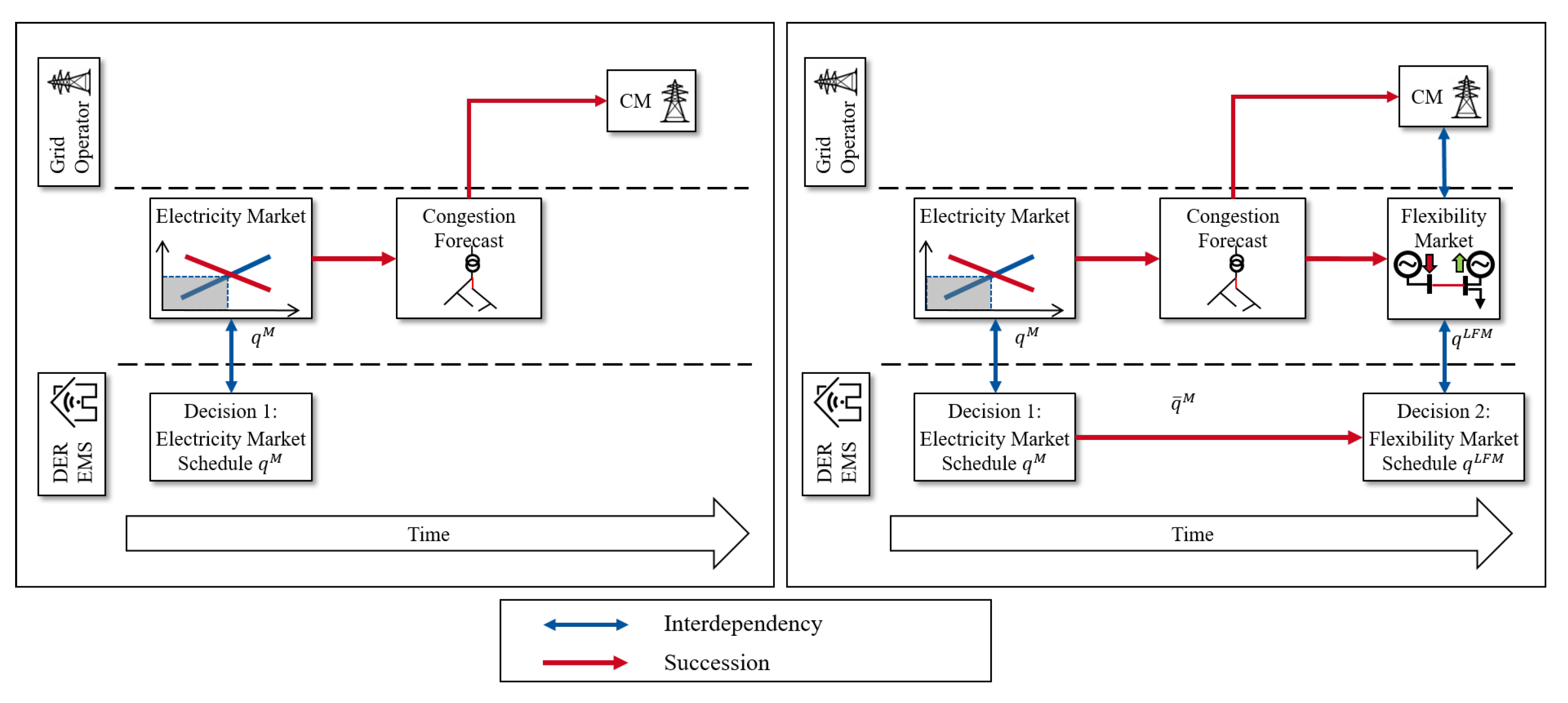
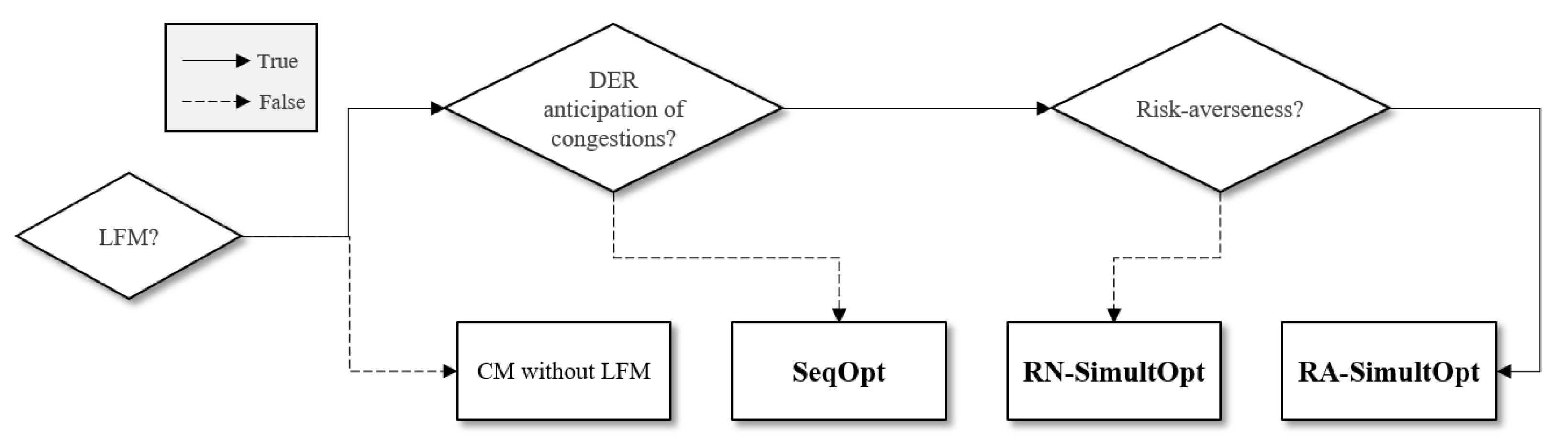
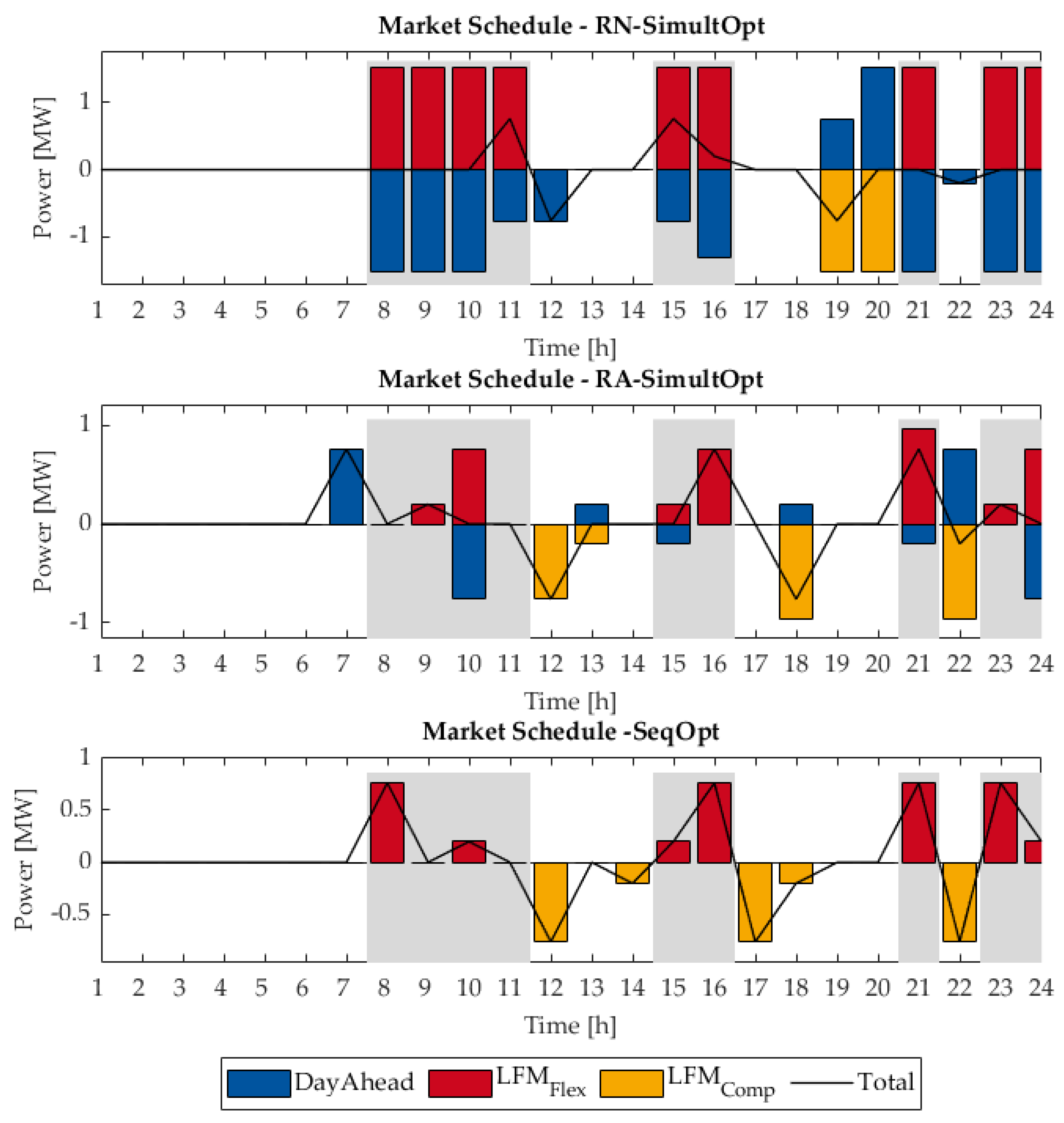
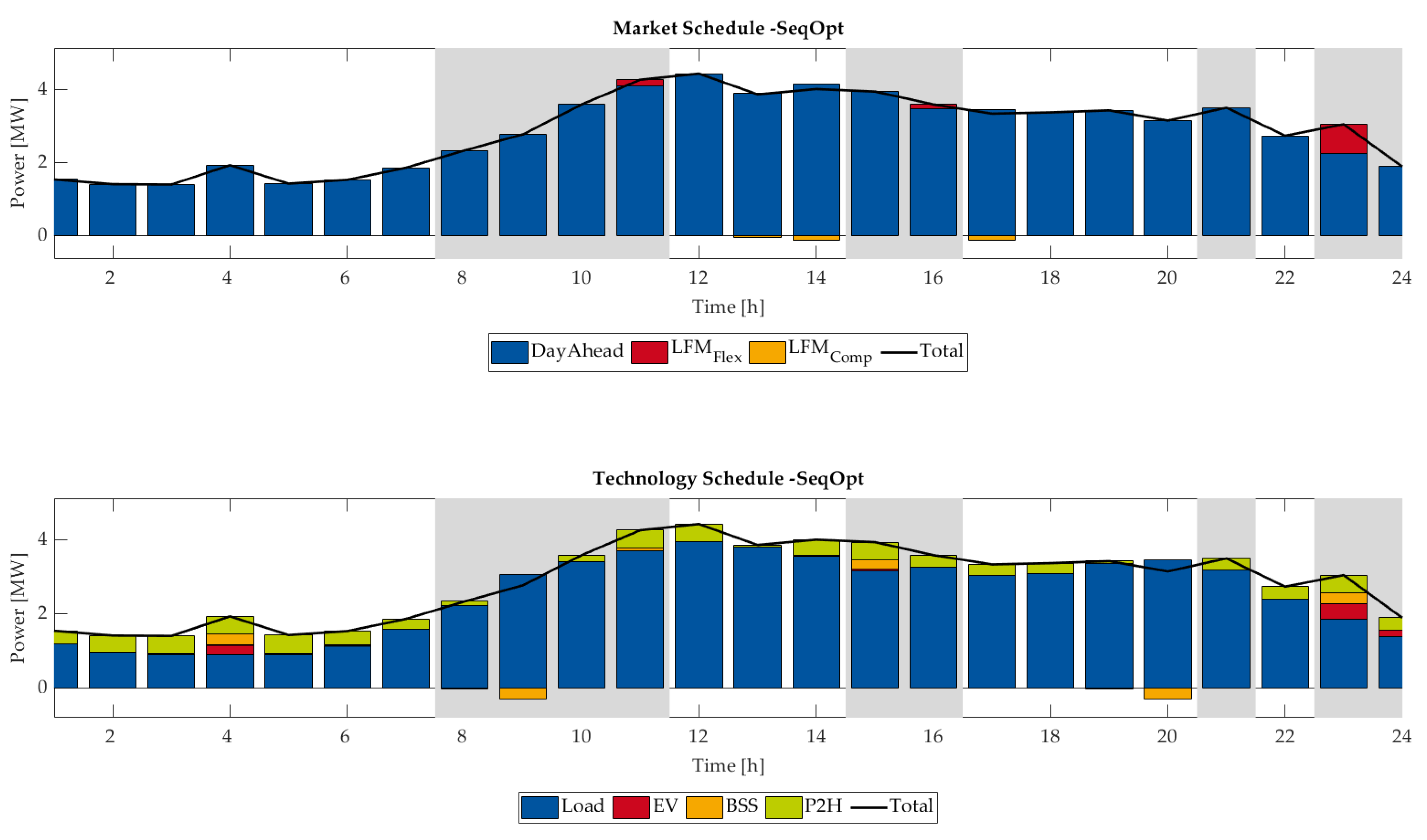
• SeqOpt: Sequential optimization in electricity markets and LFMs (as depicted in Figure 2), i.e., no anticipation of LFMs when determining electricity market schedules.
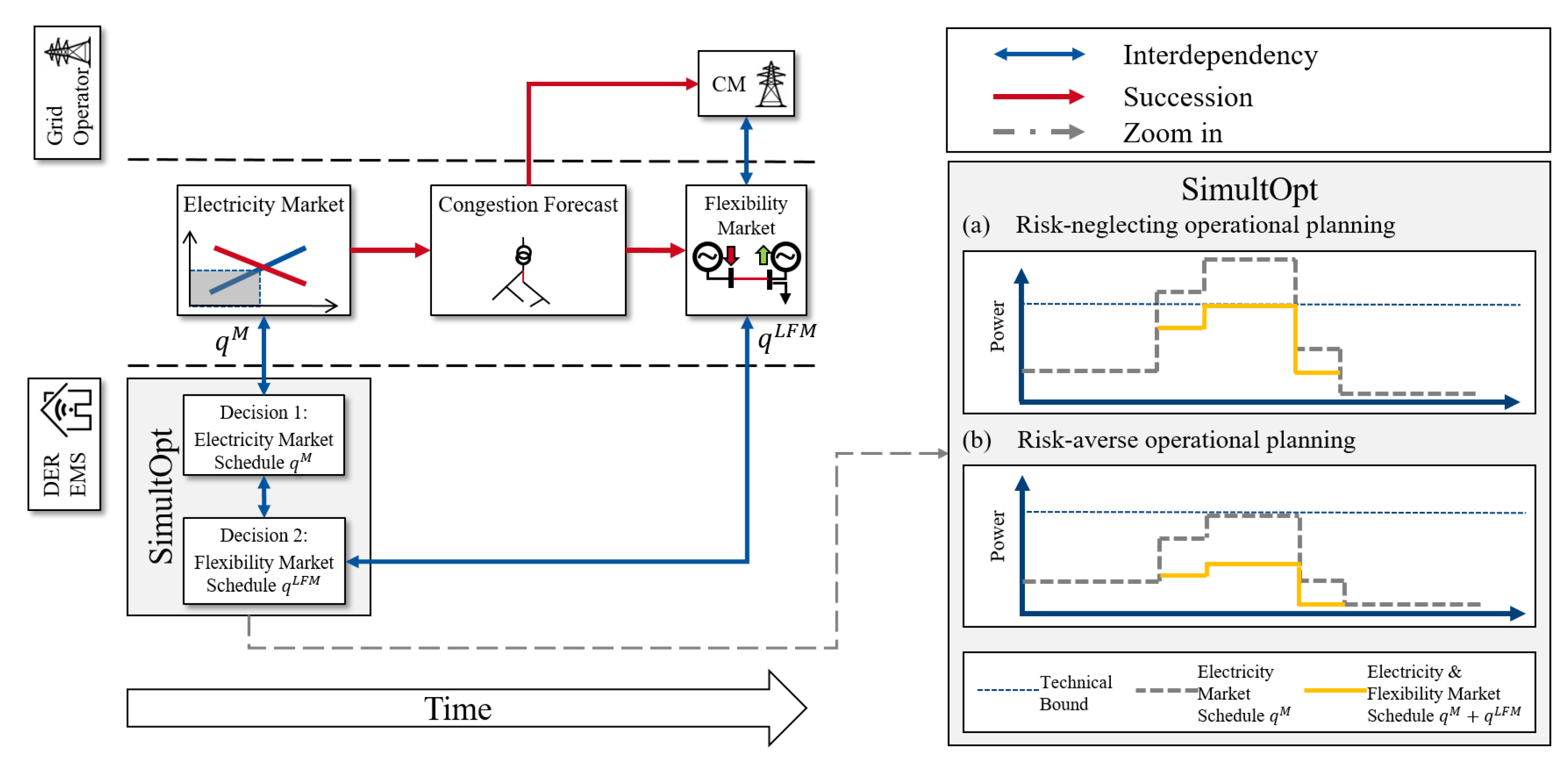
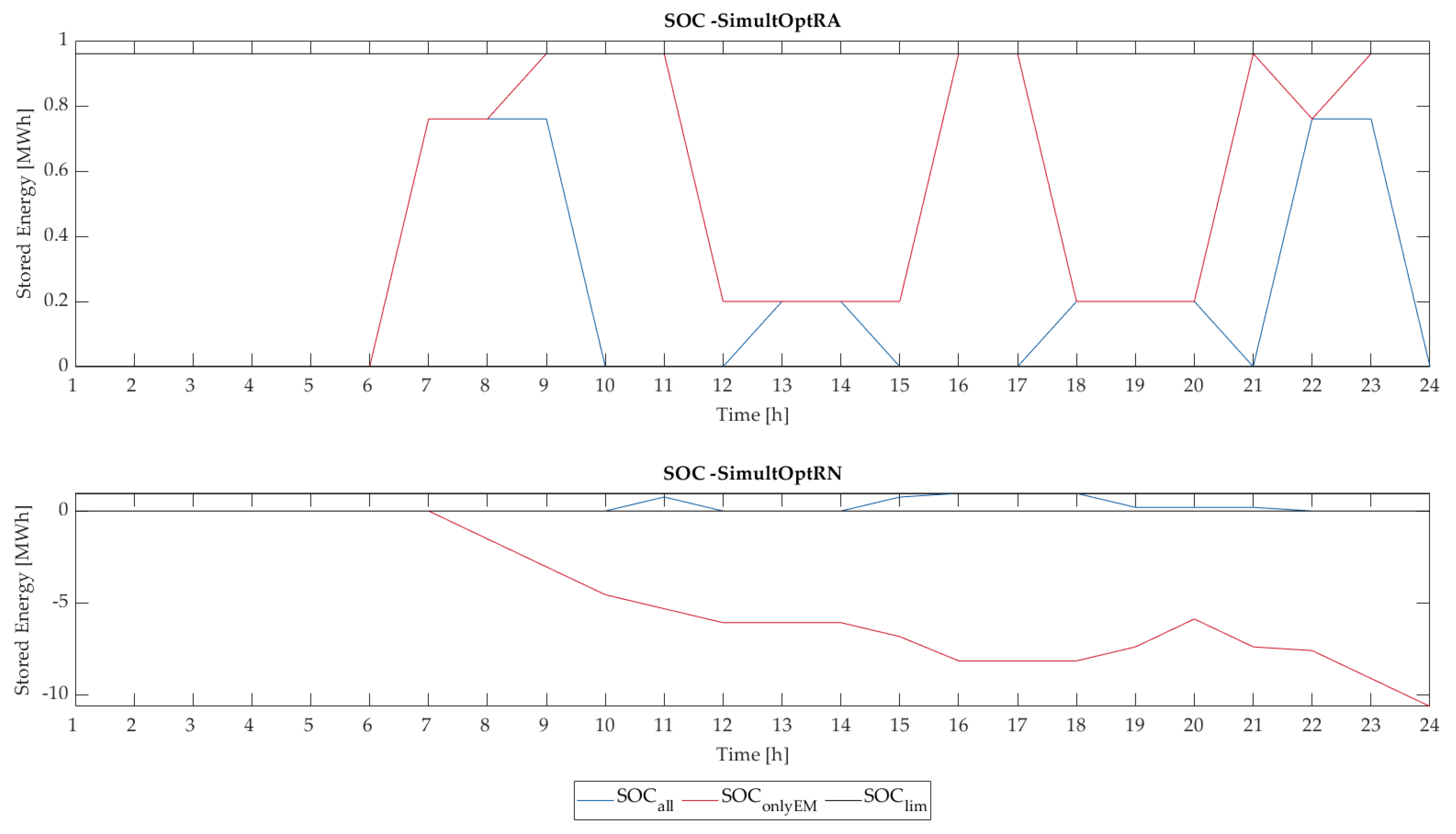
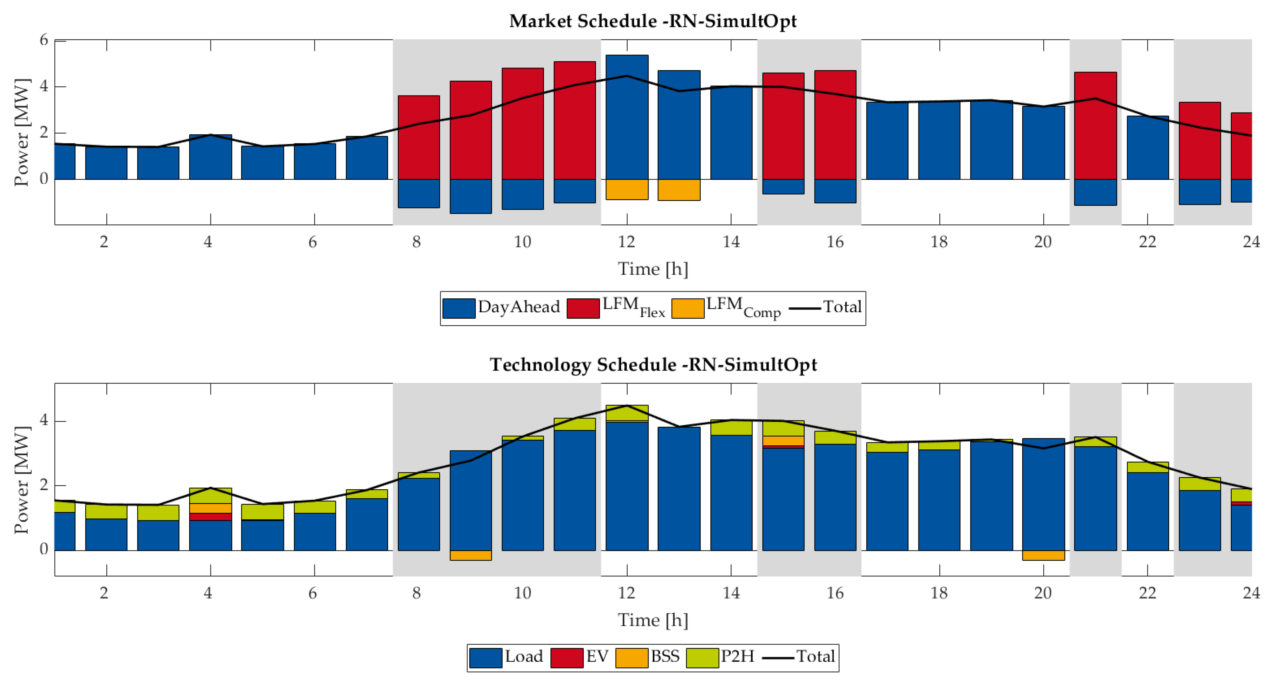
• RN-SimultOpt: Risk-neglecting anticipation of LFMs through simultaneous optimization of electricity market and LFM participation (as depicted in Figure 4a), allowing for short-selling of flexibility.
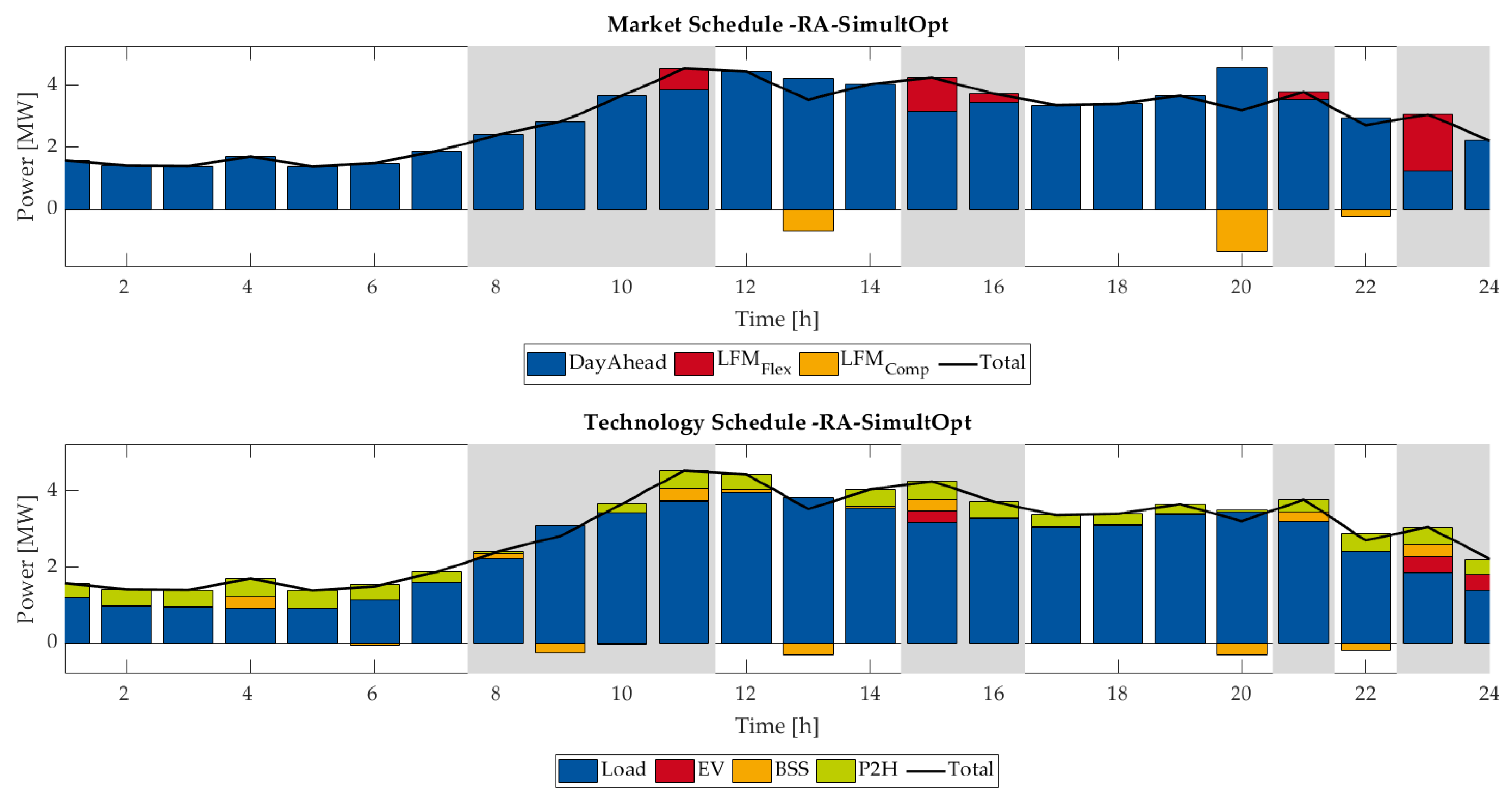
• RA-SimultOpt: Risk-averse anticipation of LFMs through simultaneous optimization of electricity and LFM participation with additional constraints for technical feasibility of the electricity market schedules (as depicted in Figure 4b), without short-selling of flexibility.

The avoidance of short-selling flexibility is considered in our paper as a risk-averse strategy because even without LFM bid activation (and thus lower profits), no imbalance costs (and no baseline deviations) occur. (When the non-activation is anticipated such that the electricity market schedule does not have to be adjusted, the non-activation has no impact on the electricity market schedule.)

This paper aims at extending the assessment approaches of market-based CM by comparing the different operational planning modes of DERs. Existing work of frameworks for the assessment of market-based CM (e.g., [19,37,38]) is progressed by explicitly evaluating the anticipatory risk-awareness of non-activation of LFM bids. An evaluation and comparison of the three limit cases of LFM operational planning can be used as the basis for ex-post assessments of LFM participation.

For this paper, we focus on a deterministic setting and do not consider uncertainties. As the term “risk” is conventionally associated with the concept of uncertainty, we have to clarify here that in this paper, the risk concept only concerns the non-activation of offered flexibility. In a deterministic setting, flexibility operators act risk-averse when they do not short-sell flexibility (even when they expect to be activated). Uncertainty reduces the potential upsides of inc-dec-gaming strategies [34,35]. However, the uncertainty of prices or activation of flexibility has to be modeled in operational planning via scenarios [39]. Therefore, the modeling of market participants’ uncertainty introduces further assumptions into mathematical modeling. These uncertainties are secondary influence factors of LFM participation and need to be distinguished from primary factors, i.e., market participants’ technology portfolios or the grid structure. To minimize modeling complexity and to increase the comprehensibility of results, we abstract from uncertainties and focus on deterministic factors for participation in LFMs.

A deterministic assessment of LFM participation not only increases comprehensibility but also simplifies the generalization of modeling assumptions. Without forecasting errors, the intraday market can be assumed to lead to equal prices as the day-ahead market. Furthermore, with perfect foresight, pay-as-bid and uniform pricing lead to equal prices since all bidding entities know the marginal prices, i.e., in a deterministic setting, both pricing approaches for LFMs are modeled equally [31]. Third, the total amount of accepted flexibility is known as ex-ante in deterministic settings, thus enabling price forecasts based on marginal costs. (Nonetheless, if flexibility offers exceed flexibility demand, it is not known which offer will be accepted.)

The rest of the paper is structured as follows. First, the electricity market participation of DERs is modeled as an EMS optimization model in Section 2 including the constraints of the individual technologies. In Section 3, the EMS optimization model is extended to model the different LFM operational planning modes. Furthermore, to take the restrictions of time-coupled flexibility of storage systems into account, the time-coupling is integrated into the operational planning and reflected in the LFM bidding structure [25]. Additionaly, the formulation of time-coupled flexibility market bids based on the operational planning results is presented. In Section 4, a hybrid LFM-clearing formulation incorporating the linear bids for LFMs as well as the grid operator’s flexibility for CM is presented. Section 5 presents the unified modeling framework incorporating the operational planning of DER operators as well as the LFM clearing process. Subsequently, a comprehensible case study is carried out to show the impact of the different operational planning modes by DER EMS.

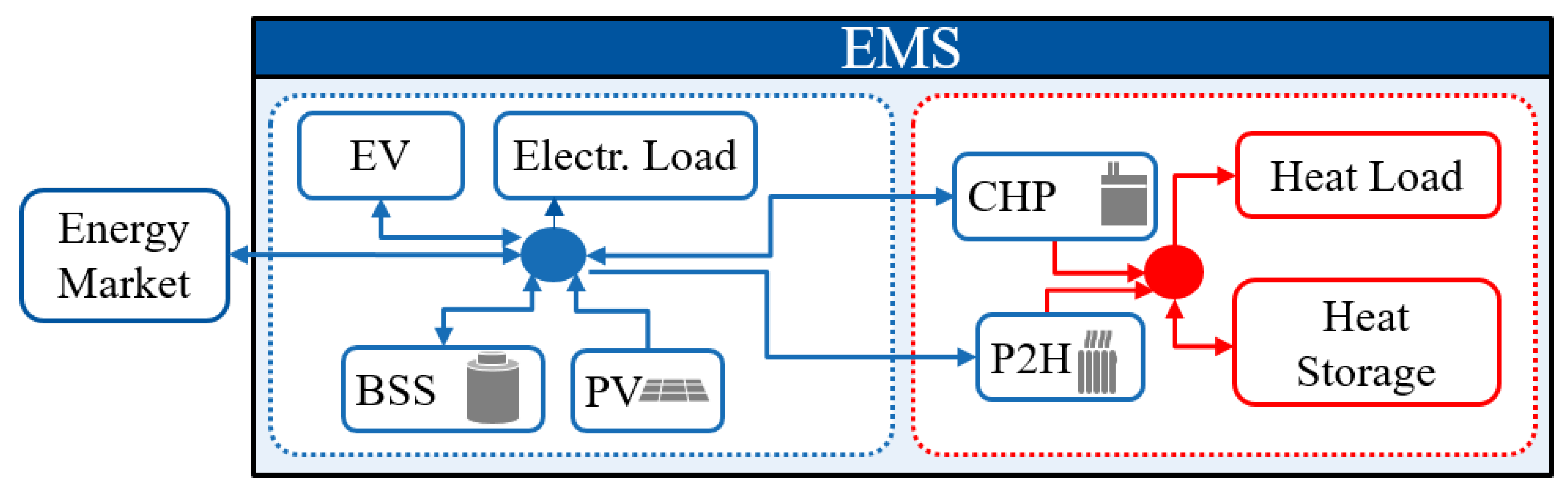
2. Energy Management System Model

The modeling of DERs is based on an EMS approach. EMS are defined here as operating systems controlling a portfolio of different technology assets such as EVs, BSS, heat pumps, etc. as depicted in Figure 5. Thus, EMS pool the different assets in order to optimize their operation and minimize energy costs. An EMS can represent the technology portfolio of a single prosumer but also the portfolio of an aggregator that considers the assets of different consumers, producers and prosumers. In the context of this paper, we assume one EMS per grid node, such that all DER at one grid node is jointly optimized. Nonetheless, with our modeling approach also several distinct EMS (aggregating different DERs) per grid node can be considered, e.g., to differentiate distinct actors.

Note that throughout this paper, decision variables are highlighted in bold. If not constrained otherwise, variables are assumed linear and unconstrained. Additionally, a nomenclature with an overview on the variables is given at the end of the paper.

In the following section, a brief overview on the modeling of the different technologies within an EMS is given. (Throughout the rest of the paper, whenever indices are omitted, the content applies for all possible mappings. For example a variable ${\mathit{x}}_t$ defined for each time step t individually can be referred to as $\mathit{x}$ if a definition applies to all time-steps equally.)

Furthermore, the coupling of those models as well as the operational planning optimization models is presented. The different technology models presented in this section are derived from the modeling approach developed in [40]. To allow for the coupling of the different technologies, for each asset i that consumes electricity, a coupling load variable ${\mathit{p}}_{i,t}^{load}$ is introduced. Likewise, for all assets producing electricity, a coupling generation variable ${\mathit{p}}_{i,t}^{gen}$ is used. The difference of the coupling variables ${\mathit{p}}_{i,t}^{load}-{\mathit{p}}_{i,t}^{gen}$ is then equal to the actual physical consumption (or generation) of the asset. The cost for buying electricity and the earnings from selling electricity are not part of the technology models but accounted explicitly. Therefore, if not presented otherwise, no operational costs occur for these technologies, i.e., ${\mathit{C}}_{i,t}=0$.

2.1. PV and Wind Power Plant Technology Models

Photovoltaic (PVs) and wind power plants (WPPs) are variable renewable energies due to their time-varying generation capacities ${\overline{P}}_{i,t}$ depending on the meteorological conditions. Nevertheless, they can also reduce their feed-in, e.g., in times of negative selling prices for electricity:

$$0\le {\mathit{p}}_{i,t}^{gen}\le {\overline{P}}_{i,t},\forall t,\forall i\in WPP\cup PV,$$

(1)

2.2. BSS Model

A BSS i can be charged (${\mathit{p}}_{i,t}^{in}$) and discharged (${\mathit{p}}_{i,t}^{out}$), both with respect to charging and discharging efficiencies ${\eta }_{i,in},{\eta }_{i,out}$ (3) and maximum charging capacities ${\overline{P}}_i^{in,max}$ (4), ${\overline{P}}_i^{out,max}$(5). The BSS SOC is limited by the battery capacities. (Note that the SOC is defined here as the absolute energy stored in contrast to the more common percentage definition.)

Furthermore, a BSS self-discharge of $(1-l_i)\%$ can be considered.

$$\begin{array}{c}{\mathit{p}}_{i,t}^{load}-{\mathit{p}}_{i,t}^{gen}={\mathit{p}}_{i,t}^{in}-{\mathit{p}}_{i,t}^{out},\forall i\in BAT,\forall t\end{array}$$

(2)

$$\begin{array}{c}{\mathit{soc}}_{i,t}={\eta }_{i,in}·{\mathit{p}}_{i,t}^{in}-{\mathit{p}}_{i,t}^{out}/{\eta }_{i,out}+{\mathit{soc}}_{i,(t-1)}·l_i,\forall i\in BAT,\forall t\end{array}$$

(3)

$$0\le {\mathit{p}}_{i,t}^{in}\le {\overline{P}}_i^{in,max},\forall i\in BAT,\forall t$$

(4)

$$0\le {\mathit{p}}_{i,t}^{out}\le {\overline{P}}_i^{out,max},\forall i\in BAT,\forall t$$

(5)

$${\underline{SOC}}_i\le {\mathit{soc}}_{i,t}\le {\overline{SOC}}_i,\forall i\in BAT,\forall t$$

(6)

2.3. P2H and Combined-Heat-and-Power Technology Model

For the coupling of the heating and the electricity sector two different base technologies are modeled: P2H technologies, i.e., heating pumps, heating rods and electric furnaces, that consume electricity to satisfy the heat demand $d^{heat}$. In contrast, combined-heat-and-power (CHP) plants generate both heat and electricity by using fuels, e.g., gas or biomass. The factor $f^{el}$ couples the electric and heating output of the system by determining the electric input ($f^{el}>0$) or electric output ($f^{el}<0$) for each unit of heat (${\mathit{p}}^h$). It is equal to the inverse of the coefficient-of-performance for P2H systems. Each heating systems is defined as a combination of base b and peak p heating technologies plus an additional heat storage. Heat pumps might have a heating rod as peak technologies, whereas it is common for CHP plants ($f^{el}<0$) to have an additional gas boiler ($f^{el}=0$) or an additional P2H system ($f^{el}>0$) for peak heat demands. For the heat storage system, $l_i^h$ is defined as the heat loss factor of storage operation and for CHP systems, ${\mathit{s}}_t$ is defined as exhaust heat.

$${\mathit{p}}_{i,t}^{load}-{\mathit{p}}_{i,t}^{gen}=f_i^{b,el}·{\mathit{p}}_{i,t}^{b,h}+f_i^{p,el}·{\mathit{p}}_{i,t}^{p,h},\forall t,\forall i\in P2H\cup CHP$$

(7)

$${\mathit{p}}_{i,t}^{b,h}+{\mathit{p}}_{i,t}^{p,h}-{\mathit{soc}}_{i,t}^h+l_i^h·{\mathit{soc}}_{i,(t-1)}^h+{\mathit{s}}_{i,t}=d_{i,t}^{heat},\forall t,\forall i\in P2H\cup CHP$$

(8)

$$0\le {\mathit{p}}_{i,t}^{b,h}\le {\overline{P}}_i^{b,el},\forall t,\forall i\in P2H\cup CHP$$

(9)

$$0\le {\mathit{p}}_{i,t}^{p,h}\le {\overline{P}}_i^{p,el},\forall t,\forall i\in P2H\cup CHP$$

(10)

$${\underline{SOC}}_i^h\le {\mathit{soc}}_{i,t}^h\le {\overline{SOC}}_i^h,\forall t,\forall i\in P2H\cup CHP$$

(11)

$$\begin{array}{c}{\mathit{s}}_{i,t}\ge 0,\forall t,\forall i\in CHP\\ {\mathit{s}}_{i,t}=0,\forall t,\forall i\in P2H\end{array}$$

(12)

The consideration of peak technologies is optional, as these systems can also exist as base-only models.

If the base or peak heating technologies are fuel-based, their fuel consumption is considered as costs for the heating operation based on the fuel prices $c^b,c^p$:

$$C_{i,t}=c^b·{\mathit{p}}_{i,t}^{b,h}+c^p·{\mathit{p}}_{i,t}^{p,h},\forall t,\forall i\in P2H\cup CHP$$

(13)

2.4. EV Model

The EV model is based on a pooling approach. This means that it can be applied to single EVs as well as a pool of cars C. The binary parameter $b_{c,t}$ defines whether a car c is parked at the EMS charging station in t.

$$b_{c,t}=\left\{\begin{array}{cc}1\hfill & \mathrm{if}\mathrm{car}\mathrm{c}\mathrm{at}\mathrm{charging}\mathrm{station}\mathrm{in}\mathrm{t}\hfill \\ 0\hfill & \mathrm{else}\hfill \end{array}\right.,\forall t,\forall c\in C$$

(14)

Arriving cars have a predefined energy-on-arrival $E_{c,t}^{arrival}$ stored in their battery and a predefined energy-on-departure demand $E_{c,t}^{departure}$. The parameters for $b_{c,t},E_{c,t}^{arrival},E_{c,t}^{departure}$ are derived from a simulation model for driving and charging behavior [41]. All cars available at the charging point are modeled as one vehicle with time-varying storage and charging capacity.

$${\mathit{p}}_{i,t}^{load}-{\mathit{p}}_{i,t}^{gen}={\mathit{p}}_{i,t}^{in}-{\mathit{p}}_{i,t}^{out},\forall i\in EV,\forall t$$

(15)

$$\begin{array}{c}{\eta }_{i,in}·{\mathit{p}}_{i,t}^{in}-{\mathit{p}}_{i,t}^{out}/{\eta }_{i,out}+{\mathit{soc}}_{i,(t-1)}\\ ={\mathit{soc}}_{i,t}-\sum _{c\in C}{b}_{c,t}·E_{c,t}^{arrival}+\sum _{c\in C}{b}_{c,t}·E_{c,t}^{departure},\forall t,\forall i\in EV\end{array}$$

(16)

$$0\le {\mathit{p}}_{i,t}^{in}\le \sum _{c\in C}{b}_{c,t}·{\overline{P}}_c^{in},\forall t,\forall i\in EV$$

(17)

$$0\le {\mathit{p}}_{i,t}^{out}\le \sum _{c\in C}{b}_{c,t}·{\overline{P}}_c^{out},\forall t,\forall i\in EV$$

(18)

$$\sum _{c\in C}{b}_{c,t}·{\underline{SOC}}_c\le {\mathit{soc}}_{i,t}\le \sum _{c\in C}{b}_{c,t}·{\overline{SOC}}_c,\forall t,\forall i\in EV$$

(19)

2.5. Electrical Load Model

The electrical load demand of the EMS $d_{i,t}^{el}$ has to be supplied and cannot be reduced:

$${\mathit{p}}_{i,t}^{load}=d_{i,t}^{el},\forall i\in D^{el},\forall t$$

(20)

Load shifting and load shedding models can be integrated into the modeling framework analogously to the formerly defined models by defining the variables ${\mathit{p}}_{i,t}^{load},{\mathit{p}}_{i,t}^{gen}$ for each time step. Load shedding models can be modeled by reformulating equality (20) as an inequality, whereas load shifting can be modeled linearly by applying the formulation given in [42]. Furthermore, load shifting and load shedding can be associated with cost parameters $C_{i,t}$.

2.6. General EMS Operational Planning

The EMS modeling approach is based on a coupling of the different technology models of the assets represented by the EMS. The overall generation and load of the assets defines the EMS schedule. First, all generation is coupled by defining two non-negative pooling variables ${\mathit{q}}_t^{g2l}$ and ${\mathit{q}}_t^{sale}$. ${\mathit{q}}_t^{g2l}$ pools all generation that is used to supply the EMS load, whereas ${\mathit{q}}_t^{sale}$ is the remaining electricity generation sold by the EMS in the electricity market.

$$\sum _{i\in A}{\mathit{p}}_{i,t}^{gen}={\mathit{q}}_t^{g2l}+{\mathit{q}}_t^{sale},\forall t$$

(21)

Analogously, the electrical load of the different assets (minus the self-supply ${\mathit{q}}_t^{g2l}$) is pooled as well to calculate the EMS purchase schedule.

$${\mathit{q}}_t^{purch}=\sum _{i\in A}{\mathit{p}}_{i,t}^{load}-{\mathit{q}}_t^{g2l},\forall t$$

(22)

$${\mathit{q}}_t^{purch},{\mathit{q}}_t^{g2l},{\mathit{q}}_t^{sale}\ge 0,\forall t$$

(23)

The EMS optimization is then defined by an optimization of operational costs depending on the electricity selling and buying prices ${\lambda }_t^S,{\lambda }_t^P$ and generation costs per asset ${\mathit{C}}_i$:

$$min\sum _t[{\mathit{q}}_t^{purch}·{\lambda }_t^P-{\mathit{q}}_t^{sale}·{\lambda }_t^S+\sum _{i\in A}{\mathit{C}}_{i,t}]$$

(24)

s.t.

$$\begin{array}{c}Assetconstraints:\mathrm{Equations}\left(1\right)–\left(20\right)\\ Assetcouplingconstraints:\mathrm{Equations}\left(21\right)–\left(23\right)\end{array}$$

(25)

The decision variables of the problem comprise the market variables ${\mathit{q}}_t^{purch},{\mathit{q}}_t^{sale}$, the coupling variable ${\mathit{q}}_t^{g2l}$, and the DER asset variables denoted in bold.

3. LFM Participation Modeling

When considering LFMs as an additional market platform, the EMS operational planning problem needs to be expanded to take the LFM into account. For this purpose, we do not only expand the operational planning formulation by the opportunity of LFM participation, but also integrate the time-coupled flexibility bids as presented in [25].

3.1. LFM Operational Planning Variables and Bid Formulation

For the integration of LFM participation into the EMS operational planning, additional variables ${\mathit{q}}^{F^{+}},{\mathit{q}}^{F^{-}}$ for positive and negative flexibility offers are introduced. Based on the LFM bid model presented in [25], storage-based flexibility is not only offering flexibility but also compensation of activated flexibility. Therefore, the variables ${\mathit{q}}^{F^{+}},{\mathit{q}}^{F^{-}}$ are defined for storage-based (time-coupled) flexibility ${\mathit{q}}^{F^{+},S},{\mathit{q}}^{F^{-},S}$ and non-storage flexibility ${\mathit{q}}^{F^{+},N},{\mathit{q}}^{F^{-},N}$ without time-coupling. Whenever flexibility ${\mathit{q}}^{F,S}$ of storage systems is activated by the DSO, the SOC of the storage system is either increased or decreased, depending on the direction (positive or negative) of flexibility. Since the SOC of storage systems is bounded, the potential of flexibility is limited, as depicted in the left part of Figure 3. To regain flexibility, a compensation ${\mathit{q}}_t^{C,S}$ of activated flexibility can be carried out in a later point of time (cf. right part of Figure 3). The activation and compensation of flexibility can be seen similar to buying and selling energy from an electrical point of view. Thus, the flexibility and its compensation will be integrated into the technology coupling constraints analogously to the variables for buying and selling electricity. The activated, but not compensated flexibility of storage systems is accounted for by using auxiliary variables ${\mathit{w}}_t^{+},{\mathit{w}}_t^{-}$. These auxiliary variables account the amount of flexibility not compensated:

$$\begin{array}{c}{\mathit{w}}_t^{+}={\mathit{w}}_{(t-1)}^{+}+{\mathit{q}}_t^{F^{+},S}-{\mathit{q}}_t^{C^{+},S},\forall t\end{array}$$

(26)

$$\begin{array}{c}{\mathit{w}}_t^{-}={\mathit{w}}_{(t-1)}^{-}+{\mathit{q}}_t^{F^{-},S}-{\mathit{q}}_t^{C^{-},S},\forall t\end{array}$$

(27)

Thus, each flexibility activation leads to an increase, whereas each compensation leads to a decrease of $\mathit{w}$. Furthermore, all variables are restricted to be non-negative:

$$\begin{array}{c}{\mathit{q}}_t^{F^{+},N},{\mathit{q}}_t^{F^{-},N},{\mathit{q}}_t^{F^{+},S},{\mathit{q}}_t^{C^{+},S},{\mathit{q}}_t^{F^{-},S},{\mathit{q}}_t^{C^{-},S},{\mathit{w}}_t^{+},{\mathit{w}}_t^{-}\ge 0,\forall t\end{array}$$

(28)

The variables of flexibility offers ${\mathit{q}}^F$ are set to zero in times of no congestion to further restrict the solution space since any offer in these time steps will not be activated by the SO anyways. While the variables for ${\mathit{w}}^{+},{\mathit{w}}^{-}$ are only used for accounting purposes, they are nevertheless an important part of the bids exchanged in the process between EMS operator and the LFM.

In the following paragraph, the definition of bids based on the operational planning results for the variables ${\mathit{q}}^F,{\mathit{q}}^C,\mathit{w}$ is presented. After determining the optimal LFM schedules (${\mathit{q}}^{F^{+},N}$,${\mathit{q}}^{F^{-},N}$, ${\mathit{q}}^{F^{+},S}$, ${\mathit{q}}^{C^{+},S}$, ${\mathit{q}}^{F^{-},S}$, ${\mathit{q}}^{C^{-},S}$, ${\mathit{w}}^{+}$, ${\mathit{w}}^{-}$), the LFM variables are evaluated to construct the LFM bid tuples. The price component of the bid is based on the expected LFM price $\pi$ also used in the operational planning process. Each bid then consists of a tuple of a price time series $\pi$, a flexibility quantity time series $\overline{Q^F}$, and, for storage-based bids, a compensation and accounting time series $\overline{Q^C},\overline{W}$. The tuples $(\pi ,\overline{Q^F},\overline{Q^C},\overline{W})$ (for time-coupled bids) and $(\pi ,\overline{Q^F})$ are build according to the following rules:

• Positive, non-storage-based flexibility:

  $$\overline{Q^{F^{+},N}}={\mathit{q}}^{F^{+},N}$$

  (29)
• Positive, storage-based bids:

  $${\overline{W}}^{+}={\mathit{w}}^{+},\overline{Q^{F^{+},S}}={\mathit{q}}^{F^{+},S},\overline{Q^{C^{+}}}={\mathit{q}}^{C^{+},S}$$

  (30)
• Negative, non-storage-based flexibility:

  $$\overline{Q^{F^{-},N}}={\mathit{q}}^{F^{-},N}$$

  (31)
• Negative, storage-based bids:

  $${\overline{W}}^{-}={\mathit{w}}^{-},\overline{Q^{F^{-},S}}={\mathit{q}}^{F^{-},S},\overline{Q^{C^{-}}}={\mathit{q}}^{C^{-},S}$$

  (32)

Within the LFM process (Section 4), the bidding tuples $(\pi ,\overline{Q^F},\overline{Q^C},\overline{W})$ are used to form constraints on the activation of flexibility. (The bidding tuples consist of temporal vectors according to the considered operational planning time horizon. The considered time horizon can be varied within the model. However, it should correspond to the time horizon of the LFM for consistency.)

By considering limits of activation, an activation without necessary compensation is prevented, ensuring technical feasibility of the executed LFM bids. Thus, within the LFM clearing process, for each bid $f\in F$ corresponding variables for activation ${\mathit{Q}}^F$, compensation ${\mathit{Q}}^C$, and accounting $\mathit{W}$ are defined analogously to their operational planning counterparts to represent the activation of these LFM bids by the market operator. The activation of the four different types of LFM bids (positive or negative, time-coupled and single-time step) is further limited by the constraints of activation, i.e., each bid f is bounded by its bid-feasible space ${\mathcal{F}}_f$. Furthermore, their activation is associated with activation costs ${\mathcal{C}}_f$. The feasible spaces ${\mathcal{F}}_f$ and costs ${\mathcal{C}}_f$ of bid activation are formally described as follows:

• Positive, non-time-coupled flexibility bids $f\in F^{+,N}$:

  $${\mathcal{F}}_f^{+,N}=\left\{{\mathit{Q}}_{f,t}^{F^{+},N}\right|0\le {\mathit{Q}}_{f,t}^{F^{+},N}\le {\overline{Q}}_{f,t}^{F^{+},N},\forall t\}$$

  (33)

  $${\mathcal{C}}_f^{+,N}=\sum _t{\pi }_{f,t}^{+}·{\mathit{Q}}_{f,t}^{F^{+},N}$$

  (34)
• Negative, non-time-coupled flexibility bids $f\in F^{-,N}$:

  $${\mathcal{F}}_f^{-,N}=\left\{{\mathit{Q}}_{f,t}^{F^{-},N}\right|0\le {\mathit{Q}}_{f,t}^{F^{-},N}\le {\overline{Q}}_{f,t}^{F^{-},N},\forall t\}$$

  (35)

  $${\mathcal{C}}_f^{-,N}=-\sum _t{\pi }_{f,t}^{-}·{\mathit{Q}}_{f,t}^{F^{-},N}$$

  (36)
• Positive, time-coupled flexibility bids $f\in F^{+,S}$:

  $$\begin{array}{c}0\le {\mathit{Q}}_{f,t}^{F^{+},S}\le {\overline{Q}}_{f,t}^{F^{+},S},\forall t\\ 0\le {\mathit{Q}}_{f,t}^{C^{+}}\le {\overline{Q}}_{f,t}^{C^{+}},\forall t\end{array}$$

  (37)

  $$\begin{array}{c}{\mathit{W}}_{t,f}^{+}={\mathit{W}}_{(t-1),f}^{+}+{\mathit{Q}}_{f,t}^{F^{+},S}-{\mathit{Q}}_{f,t}^{C^{+}},\forall t\\ 0\le {\mathit{W}}_{t,f}^{+}\le {\overline{W}}^{+},\forall t\end{array}$$

  (38)

  $${\mathcal{F}}_f^{+,S}=\{{\mathit{Q}}_{f,t}^{F^{+},S},{\mathit{Q}}_{f,t}^{C^{+}},{\mathit{W}}_{t,f}^{+}|\mathrm{Equations}\left(37\right)\mathrm{and}\left(38\right),\forall t\}$$

  (39)

  $${\mathcal{C}}_f^{+,S}=\sum _t{\pi }_{f,t}^{+}·{\mathit{Q}}_{f,t}^{F^{+},S}-{\pi }_{f,t}^{-}·{\mathit{Q}}_{f,t}^{C^{+},S}$$

  (40)
• Negative, time-coupled flexibility bids $f\in F^{-,S}$:

  $$\begin{array}{c}0\le {\mathit{Q}}_{f,t}^{F^{-},S}\le {\overline{Q}}_{f,t}^{F^{-},S},\forall t\\ 0\le {\mathit{Q}}_{f,t}^{C^{-}}\le {\overline{Q}}_{f,t}^{C^{-}},\forall t\end{array}$$

  (41)

  $$\begin{array}{c}{\mathit{W}}_{t,f}^{-}={\mathit{W}}_{(t-1),f}^{-}+{\mathit{Q}}_{f,t}^{F^{-},S}-{\mathit{Q}}_{f,t}^{C^{-}},\forall t\\ 0\le {\mathit{W}}_{t,f}^{-}\le {\overline{W}}^{-},\forall t\end{array}$$

  (42)

  $${\mathcal{F}}_f^{-,S}=\{{\mathit{Q}}_{f,t}^{F^{-},S},{\mathit{Q}}_{f,t}^{C^{-}},{\mathit{W}}_{t,f}^{-}|\mathrm{Equations}\left(41\right)\mathrm{and}\left(42\right),\forall t\}$$

  (43)

  $${\mathcal{C}}_f^{-,S}=\sum _t-{\pi }_{f,t}^{-}·{\mathit{Q}}_{f,t}^{F^{-},S}+{\pi }_{f,t}^{+}·{\mathit{Q}}_{f,t}^{C^{-},S}$$

  (44)

The limitations of the accounting variables in (38) and (42) are based on constraints (26) and (27). They ensure that at most the amount of activated flexibility can be compensated. Furthermore, these constraints prevent an unlimited activation of flexibility without compensation.

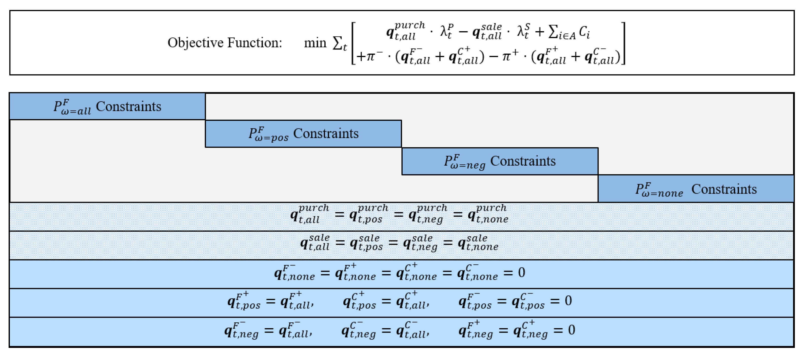
3.2. EMS LFM Operational Planning

For the LFM participation, the EMS coupling constraints are expanded to take flexibility offerings into account. Based on an active sign convention, negative flexibility $F^{-}$ refers to additional load and positive flexibility $F^{+}$ refers to additional generation. The assets are categorized as storage-based technologies $A^S$ that are subject to time-coupling constraints such as states-of-charge, and non-storage based technologies $A^N$. To take the need for compensation energy $q^C$ for storage-based systems into account, the coupling constraints are differentiated between storage-based technologies $A^S$ (46) and non-storage-based technologies $A^N$ (45). The coupling constraint (47) enables a supply from storage-based technologies to non-storage-based technologies and vice versa.

$$\sum _{i\in A^N}{\mathit{p}}_{i,t}^{gen}={\mathit{q}}_t^{N,g2l}+{\mathit{q}}_t^{sale,N}+{\mathit{q}}_t^{F^{+},N}+{\mathit{id}}_t,\forall t$$

(45)

$$\sum _{i\in A^S}{\mathit{p}}_{i,t}^{gen}={\mathit{q}}_t^{S,g2l}+{\mathit{q}}_t^{sale,S}+{\mathit{q}}_t^{F^{+},S}+{\mathit{q}}_t^{C^{-},S},\forall t$$

(46)

$${\mathit{q}}_t^{N,g2l}+{\mathit{q}}_t^{S,g2l}={\mathit{q}}_t^{g2l,N}+{\mathit{q}}_t^{g2l,S},\forall t$$

(47)

$${\mathit{q}}_t^{purch,N}+{\mathit{q}}_t^{F^{-},N}=\sum _{i\in A^N}{\mathit{p}}_{i,t}^{load}-{\mathit{q}}_t^{g2l,N}-{\mathit{id}}_t,\forall t$$

(48)

$${\mathit{q}}_t^{purch,S}+{\mathit{q}}_t^{F^{-},S}+{\mathit{q}}_t^{C^{+},S}=\sum _{i\in A^S}{\mathit{p}}_{i,t}^{load}-{\mathit{q}}_t^{g2l,S},\forall t$$

(49)

$${\mathit{q}}_t^{purch,N},{\mathit{q}}_t^{purch,S},{\mathit{q}}_t^{N,g2l},{\mathit{q}}_t^{S,g2l},{\mathit{q}}_t^{g2l,N},{\mathit{q}}_t^{g2l,S},{\mathit{q}}_t^{sale,N},{\mathit{q}}_t^{sale,S}\ge 0,{\mathit{id}}_t\in \mathbb{R},\forall t$$

(50)

The variable ${\mathit{id}}_t$ is only introduced to explicitly allow for an energy shift from the spot market to the LFM or vice versa to model inc-dec-gaming [31]. The optional introduction of the variable ${\mathit{id}}_t$ allows for an artificial increase of inc-dec-gaming potential by the EMS. The extra variable ${\mathit{id}}_t$ is unnecessary for storage-based technologies due to the distinction between the generation and load variables ${\mathit{p}}_{i,t}^{gen},{\mathit{p}}_{i,t}^{load}$ and the physical input and output variables ${\mathit{p}}_{i,t}^{out},{\mathit{p}}_{i,t}^{in}$ in the coupling constraints (2), (7), (15) respectively. This decoupling of physical generation and load from the market schedule variables allows for the same effect as the variable ${\mathit{id}}_t$ implicitly. Since this decoupling is not possible for one-directional technologies with either generation or load, the variable ${\mathit{id}}_t$ is introduced explicitly. However, ${\mathit{id}}_t$ can be omitted, for example if only electrical loads exist as non-storage bases technologies as in that case a further increase of inc-dec-gaming through ${\mathit{id}}_t$ is unlikely in reality. Nonetheless, it is provided in this formulation for completeness.

The overall problem LFM participation problem $P^F$ is defined by the optimization model (51) and (52).

$$\begin{array}{c}min{\displaystyle \sum _t}[({\mathit{q}}_t^{purch,N}+{\mathit{q}}_t^{purch,S})·{\lambda }_t^P-({\mathit{q}}_t^{sale,N}+{\mathit{q}}_t^{sale,S})·{\lambda }_t^S+{\displaystyle \sum _{i\in A}}{\mathit{C}}_{i,t}\\ +{\pi }_t^{-}·({\mathit{q}}_t^{F^{-},N}+{\mathit{q}}_t^{F^{-},S}+{\mathit{q}}_t^{C^{+},S})-{\pi }_t^{+}·({\mathit{q}}_t^{F^{+},N}+{\mathit{q}}_t^{F^{+},S}+{\mathit{q}}_t^{C^{-},S})]\end{array}$$

(51)

s.t.

$$\begin{array}{c}Assetconstraints:\mathrm{Equations}\left(1\right)–\left(20\right)\\ LFMbidconstraints:\mathrm{Equations}\left(26\right)–\left(28\right)\\ LFMassetcouplingconstraints:\mathrm{Equations}\left(45\right)–\left(50\right)\end{array}$$

(52)

If a subset of technologies is to be excluded from the LFM participation, the coupling constraints (21)–(23) can be introduced for those technologies and added to the optimization problem. They are thus not coupled to the LFM constraints. This is the case for renewable plants (WPP, PV) in the hybrid CM regime. WPPs and PV can be considered for the operational planning in electricity markets, but for CM, they are curtailed by the DSO directly based on regulatory costs.

3.3. Risk-Averse Operational Planning for LFMs

The LFM participation formulation $P^F$ ((51) and (52)) assumes perfect foresight and does not take into account the possibility of non-activation of flexibility offered in the LFM. While electricity spot market bids can be assumed as cleared-as-bid for small-scale prosumers, the non-activation of offered flexibility for CM is a significant risk if not considered within the operational planning. If the non-activation of flexibility is not considered as a technical constraint, the asset operator has to buy balancing energy due to the technical asset constraints and might be subject to sanctions by the LFM operator. To prevent that case, the optimization problem $P^F$ ((51) and (52)) is expanded to take into account the technical limit scenarios $\omega$ of flexibility activation. The limit cases are

• $\omega =none$: no LFM consideration
• $\omega =pos$: only positive LFM participation
• $\omega =neg$: only negative LFM participation
• $\omega =all$: both positive and negative LFM participation

Each limit scenario $\omega$ is a representation of the base optimization problem $P^F$. The distinct consideration of scenarios for positive and negative flexibility offers prevents a mixed accounting that would cancel positive and negative activation out. By duplication and manipulation of the base problem $P^F$ and coupling of the scenarios, the technical limit scenarios can be taken into account simultaneously.

The bound manipulation for the limit scenarios is described in the following. For the case of no LFM participation, the LFM variables are set to zero:

$${\mathit{q}}_{t,none}^{F^{+},N}={\mathit{q}}_{t,none}^{F^{-},N}={\mathit{q}}_{t,none}^{F^{+},S}={\mathit{q}}_{t,none}^{C^{+},S}={\mathit{q}}_{t,none}^{F^{-},S}={\mathit{q}}_{t,none}^{C^{-},S}=0,\forall t$$

(53)

For the positive case, only negative LFM variables are set to zero:

$${\mathit{q}}_{t,pos}^{F^{-},N}={\mathit{q}}_{t,pos}^{F^{-},S}={\mathit{q}}_{t,pos}^{C^{-},S}=0,\forall t$$

(54)

For the negative case, the positive LFM variables are set to zero:

$${\mathit{q}}_{t,neg}^{F^{+},N}={\mathit{q}}_{t,neg}^{F^{+},S}={\mathit{q}}_{t,neg}^{C^{+},S}=0,\forall t$$

(55)

The electricity market schedule is defined equal in all cases to generate a feasible electricity market schedule for a possible levels of LFM activation:

$$\begin{array}{c}{\mathit{q}}_{t,\omega }^{purch,N}={\mathit{q}}_{t,all}^{purch,N},\omega \in \{none,pos,neg\},\forall t\\ {\mathit{q}}_{t,\omega }^{purch,S}={\mathit{q}}_{t,all}^{purch,S},\omega \in \{none,pos,neg\},\forall t\\ {\mathit{q}}_{t,\omega }^{sale,N}={\mathit{q}}_{t,all}^{sale,N},\omega \in \{none,pos,neg\},\forall t\\ {\mathit{q}}_{t,\omega }^{sale,S}={\mathit{q}}_{t,all}^{sale,S},\omega \in \{none,pos,neg\},\forall t\end{array}$$

(56)

Furthermore, the “$\omega =all$“ scenario is used as an accounting scenario that assumes full activation of flexibility:

$$\begin{array}{c}{q}_{t,pos}^{F^{+},N}=q_{t,all}^{F^{+},N},{\mathit{q}}_{t,pos}^{F^{+},S}={\mathit{q}}_{t,all}^{F^{+},S},{\mathit{q}}_{t,pos}^{C^{+},S}={\mathit{q}}_{t,all}^{C^{+},S},\forall t\end{array}$$

(57)

$$\begin{array}{c}{q}_{t,neg}^{F^{-},N}=q_{t,all}^{F^{-},N},{\mathit{q}}_{t,neg}^{F^{-},S}={\mathit{q}}_{t,all}^{F^{-},S},{\mathit{q}}_{t,neg}^{C^{-},S}={\mathit{q}}_{t,all}^{C^{-},S},\forall t\end{array}$$

(58)

To prevent a distortion of costs and earnings, they are only taken into account for the “$\omega =all$“ scenario since it considers all flexibility offering, both positive and negative. Then, the complete formulation $P^{F,RA}$ for the risk-averse case based on the scnearios $\omega$ is given as follows:

$$\begin{array}{c}min{\displaystyle \sum _t}[({\mathit{q}}_{t,all}^{purch,N}+{\mathit{q}}_{t,all}^{purch,S})·{\lambda }_t^P-({\mathit{q}}_{t,all}^{sale,N}+{\mathit{q}}_{t,all}^{sale,S})·{\lambda }_t^S+{\displaystyle \sum _{i\in A}}{\mathit{C}}_{i,t,all}\\ +{\pi }_t^{-}·({\mathit{q}}_{t,all}^{F^{-},N}+{\mathit{q}}_{t,all}^{F^{-},S}+{\mathit{q}}_{t,all}^{C^{+},S})-{\pi }_t^{+}·({\mathit{q}}_{t,all}^{F^{+},N}+{\mathit{q}}_{t,all}^{F^{+},S}+{\mathit{q}}_{t,all}^{C^{-},S})]\end{array}$$

(59)

s.t.

$$\begin{array}{c}\omega \in \{all,none,pos,neg\}\left\{\begin{array}{c}\omega -Assetconstraints:\mathrm{Equations}\left(1\right)–\left(20\right)\hfill \\ \omega -LFMbidconstraints:\mathrm{Equations}\left(26\right)–\left(28\right)\hfill \\ \omega -LFMassetcouplingconstraints:\mathrm{Equations}\left(45\right)–\left(50\right)\hfill \end{array}\right.\end{array}$$

(60)

$$Scnearioconstraints:\mathrm{Equations}\left(53\right)–\left(58\right)$$

(61)

The overall problem structure is also depicted in Figure 6.

By setting the spot market schedules ${\mathit{q}}^{purch},{\mathit{q}}^{sale}$ equal in all limit scenarios of the risk-averse operational planning, and considering a scenario with no LFM participation, the fulfilment of the supply task ($d^{el},d^{heat},etc.$) is ensured. Furthermore, by considering the extreme cases of flexibility activation we ensure that for every level of flexibility activation in the LFM, the resulting LFM schedule (${\mathit{q}}^{F+},{\mathit{q}}^{F-},{\mathit{q}}^{C+},{\mathit{q}}^{C-},·$) is technically feasible for the original problem $P^F$. This is facilitated through the emulation of the operational planning constraints (26) and (27) by the flexibility bid constraints (38) and (42). As demonstrated in [25], the linear modeling of DER technologies in Section 3, together with the consideration of extreme cases of flexibility activation in $P^{F,RA}$ and the formulation of bids (in Equations (33), (39), (35), and (43)) guarantee technical flexibility of the bidding DER technologies for all possible bid activation levels by the LFM operator.

For the sequential case SeqOpt, the first optimization problem (24) and (25) determines the market schedule ${\overline{q}}^M={\mathit{q}}^{purch}-{\mathit{q}}^{sale}$ independently of LFMs. Then, the sale and purchase variables are set equal to the market schedule for the problem $P^F$. The modified problem $P^F\left({\overline{q}}^M\right)$ is subsequently solved to calculate the optimal LFM schedule.

4. LFM Clearing Formulation

For the LFM modeling, we assume a process similar to the day-ahead congestion forecast and redispatch or curtailment process currently carried out by transmission and distribution system operators for CM. If the forecasted power flow $S_{l,t}^0$ on a line l exceeds the nominal line rating ${\overline{S}}_l$, the system operator has to carry out CM measures, e.g., curtailment of renewable generation. For simplicity and because we consider radial distribution grids, in this paper we only consider congestions based on thermal line overloads and neglect further CM aspects such as the (n-1)-criterion. Furthermore, as proposed in [3], we assume LFMs as an additional, market-based CM measure to integrate load-based flexibility into the otherwise cost-based CM procedure. The LFM clearing process therefore can be modeled as a hybrid CM process combining "classical" CM (cf. [29]) and the usage of distributed, market-based flexibility bids.

The overall objective comprises a cost minimization by the system operator with curtailment costs for renewables based on compensations for lost earnings and market premia. The cost-based redispatch and curtailment measures $\Delta P$ are associated with cost parameters, whereas the flexibility offered in the LFM is associated with a price bid component $\pi$. Furthermore, we assume here that the balancing of schedules is carried out by the system operator as part of the CM. For simplicity, the cost for balancing are here assumed to be equal to (intraday) electricity market prices.

$$\begin{array}{c}min{\displaystyle \sum _t}[\underset{Conv.cong.mngmt.}{\underbrace{{\displaystyle \sum _{p\in B}}{c}_p^{+}·\Delta {\mathit{P}}_{p,t}^{+}+c_p^{-}·\Delta {\mathit{P}}_{p,t}^{-}}}\\ +\sum _{f\in F}\underset{pos.LFM}{\underbrace{{\pi }_{f,t}^{+}·({\mathit{Q}}_{f,t}^{F^{+},N}+{\mathit{Q}}_{f,t}^{F^{+},S}+{\mathit{Q}}_{f,t}^{C^{-},S})}}-\underset{neg.LFM}{\underbrace{{\pi }_{f,t}^{-}·({\mathit{Q}}_{f,t}^{F^{-},N}+{\mathit{Q}}_{f,t}^{F^{-},S}+{\mathit{Q}}_{f,t}^{C^{+},S})}}]\end{array}$$

(62)

For direct current-based power flow studies, the impact of a flexibility measure on a congestion can be assessed with the help of linear power transfer distribution factors ${\rho }_{l,n}$ that represent the per-unit active power flow on line l for an power injection at grid node n. Each conventional flexibility as well as flexibility bids f are mapped to grid nodes n within the line constraints (63), thus coupling the assets to power flows. Then, the congestion constraints can be described as follows:

$$\begin{array}{c}-{\overline{S}}_l-S_{l,t}^0\le \\ {\displaystyle \sum _{n\in N}}{\rho }_{l,n}·[{\displaystyle \sum _{p\in B\left(n\right)}}(\Delta {\mathit{P}}_{p,t}^{+}-\Delta {\mathit{P}}_{p,t}^{-})\\ +{\displaystyle \sum _{f\in F\left(n\right)}}({\mathit{Q}}_{f,t}^{F^{+},N}+{\mathit{Q}}_{f,t}^{F^{+},S}+{\mathit{Q}}_{f,t}^{C^{-},S}-{\mathit{Q}}_{f,t}^{F^{-},N}-{\mathit{Q}}_{f,t}^{F^{-},S}-{\mathit{Q}}_{f,t}^{C^{+},S})]\\ \le {\overline{S}}_l-S_{l,t}^0:{\pi }_{l,t}^{Cong},\forall t,\forall l\in L\end{array}$$

(63)

Additionally, to keep the system balance intact, total activation of positive and negative flexibility has to be equal:

$$\begin{array}{c}{\displaystyle \sum _{p\in B}}\Delta {\mathit{P}}_{p,t}^{+}+\sum _{f\in F}({\mathit{Q}}_{f,t}^{F^{+},N}+{\mathit{Q}}_{f,t}^{F^{+},S}+{\mathit{Q}}_{f,t}^{C^{-},S})\\ ={\displaystyle \sum _{p\in B}}\Delta {\mathit{P}}_{p,t}^{-}+\sum _{f\in F}({\mathit{Q}}_{f,t}^{F^{-},N}+{\mathit{Q}}_{f,t}^{F^{-},S}+{\mathit{Q}}_{f,t}^{C^{+},S}):{\pi }_t^{Bal},\forall t\end{array}$$

(64)

The dual variables ${\pi }_{l,t}^{Cong},{\pi }_t^{Bal}$ of the line and balance constraints are used in the process of determining nodal prices (cf. Section 5). The conventional flexibility $\Delta \mathit{P}$ itself is constrained and depending on the operating point $P^0$ before CM.

$$\begin{array}{c}0\le \Delta {\mathit{P}}_{p,t}^{+}\le {\overline{P}}_p-P_{p,t}^0,\forall t,\forall p\in B\\ 0\le \Delta {\mathit{P}}_{p,t}^{-}\le P_{p,t}^0,\forall t,\forall p\in B\end{array}$$

(65)

The constraints in (65) are simplified asset constraints of redispatch and CM operations. The constraints can be expanded by more complex constraints, e.g., for thermal power plants [43].

The feasible space ${\mathcal{F}}_f$ for each LFM bid f limits the possible activation of flexibility by the market operator.

$$\begin{array}{c}{\mathit{Q}}_{f,t}^{F^{+},N}\in {\mathcal{F}}_f^{+,N},\forall t,\forall f\in F^{F^{+},N}\\ {\mathit{Q}}_{f,t}^{F^{-},N}\in {\mathcal{F}}_f^{-,N},\forall t,\forall f\in F^{F^{-},N}\\ {\mathit{Q}}_{f,t}^{F^{+},S},{\mathit{Q}}_{f,t}^{C^{+},S},{\mathit{W}}_{f,t}^{+}\in {\mathcal{F}}_f^{+,S},\forall t,\forall f\in F^{F^{+},S}\\ {\mathit{Q}}_{f,t}^{F^{-},S},{\mathit{Q}}_{f,t}^{C^{-},S},{\mathit{W}}_{f,t}^{-}\in {\mathcal{F}}_f^{-,S},\forall t,\forall f\in F^{F^{-},S}\end{array}$$

(66)

As explained in Section 3, the usage of the accounting variables $\mathit{W}$ ensures that at most the amount of activated flexibility can be compensated. Furthermore, an unlimited activation of flexibility without compensation is prevented.

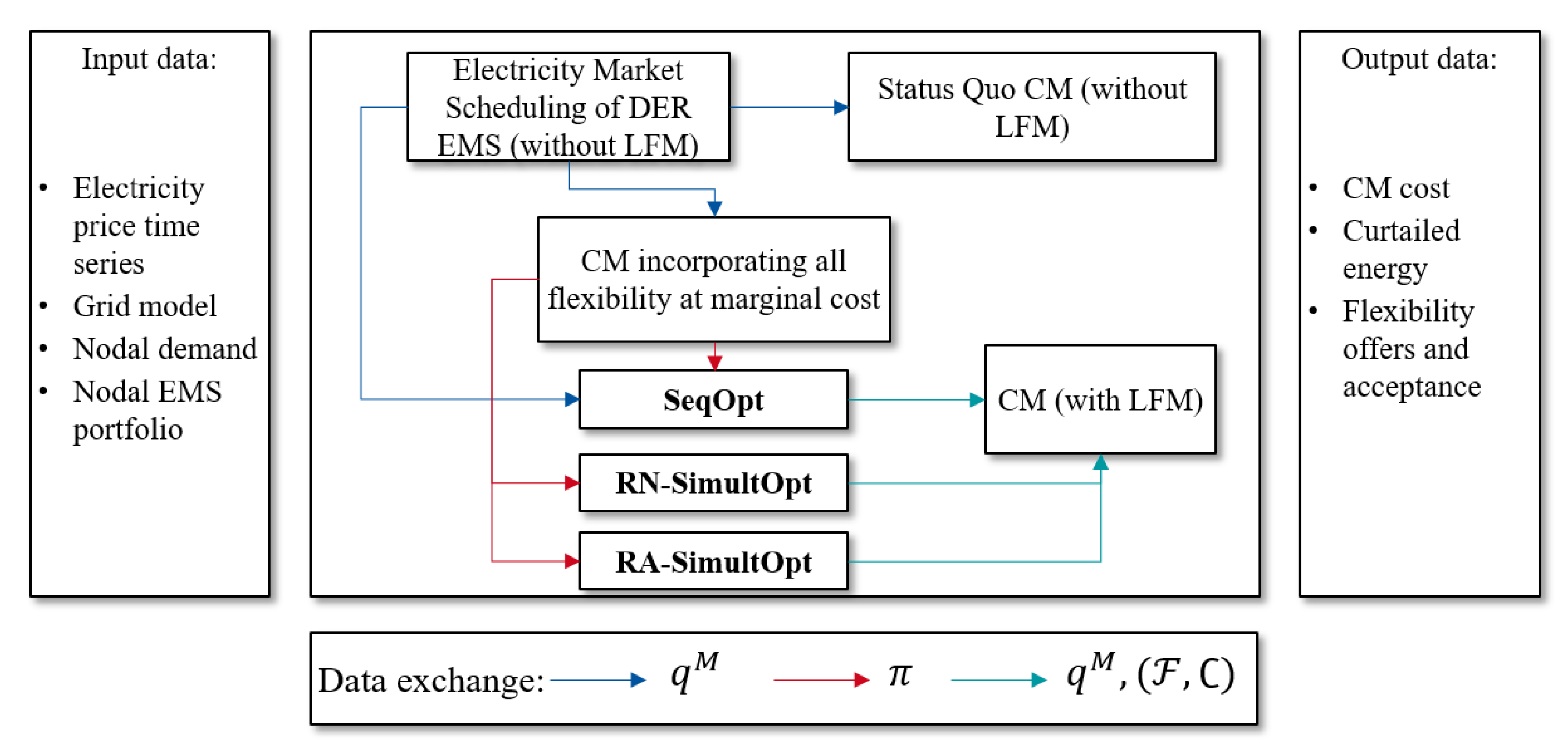
5. Integrated Modeling Framework of Operational Planning and LFM Operation

As described in Section 4, LFMs are used as a supplement to cost-based CM in this paper. Thus, in distribution systems, the system operator can choose between curtailment of renewable plants, grid measures and using offered flexibility by DERs. Therefore, wind power plants and PV plants do not participate in the LFM. Furthermore, flexibility offered by DERs has to be cheaper than the system operator’s opportunity costs for CM in order to be activated.

For the assessment of LFM participation, the CM costs for the different assumptions of how operational planning is carried out by DER operators trough their EMS have to be compared to a benchmark without LFMs (which represents the status quo).

Thus, four different cases can be identified as depicted in Figure 7 and modeled within our framework:

• the benchmark case without LFMs;
• sequential decision making in electricity and LFMs (SeqOpt $P^F\left({\overline{q}}^M\right)$);
• anticipation of the LFM with negligence of LFM risks of non-activation (Risk-neglecting RN-SimultOpt $P^F$);
• anticipation of the LFMs with risk-averse operational planning (Risk-averse RA-SimultOpt $P^{F,RA}$)

The modeling of these four cases is oriented on the process diagrams in Figure 2 and Figure 4.

For the benchmark case without consideration of LFMs, first the EMS operational planning without LFM participation (24) and (25) is carried out. Subsequently, line congestions are identified and the optimal CM is calculated by simply considering the hybrid model (63)–(65) without any LFM bids:

$$\begin{array}{c}min{\displaystyle \sum _t}{\displaystyle \sum _{p\in B}}{c}_p^{+}·\Delta {\mathit{P}}_{p,t}^{+}+c_p^{-}·\Delta {\mathit{P}}_{p,t}^{-}\end{array}$$

(67)

s.t.

$$\begin{array}{c}-{\overline{S}}_l-S_{l,t}^0\le {\displaystyle \sum _{n\in N}}{\rho }_{l,n}·\left[{\displaystyle \sum _{p\in B\left(n\right)}}(\Delta {\mathit{P}}_{p,t}^{+}-\Delta {\mathit{P}}_{p,t}^{-})\right]\le {\overline{S}}_l-S_{l,t}^0,\forall t,\forall l\in L\end{array}$$

(68)

$$\mathrm{Equation}\left(65\right)$$

(69)

$$\begin{array}{c}{\displaystyle \sum _{p\in B}}\Delta {\mathit{P}}_{p,t}^{+}={\displaystyle \sum _{p\in B}}\Delta {\mathit{P}}_{p,t}^{-},\forall t\end{array}$$

(70)

The nodal prices of the benchmark CM correspond to the marginal costs and thus nodal willingness to pay for additional flexibility of the system operator.

However, if the amount of flexibility offers is high enough to resolve the congestions without the usage of any conventional CM flexibility, i.e., the supply exceeds the demand, the flexibility operators will start to compete on their prices. With perfect competition, these prices will converge to the marginal costs of the underlying flexibility. Due to this price convergence, system cost minimization models are an established approach to model competitive markets [44]. (For example in the case of distribution systems, if all congestions could be solved with BSSs, only costs for balancing would arise. Then, the LFM prices would converge to balancing prices.)

As a result, the LFM or hybrid CM with perfect competition can be modeled as an optimal power flow problem considering all flexibility at marginal or regulatory cost.

As outlined in [1], if the same flexibility is available in the electricity market as well as the cost-based CM, the CM result is independent of of the actual electricity market result and will always lead to the same market outcome. (This assumption only holds in cases without start-up and shut-down costs. If thermal power plants with start-up costs are considered, the CM result will become dependent on which power plant is online after electricity market clearing. Furthermore, this only holds for a cost-minimal CM in contrast to a minimization of redispatch volumes. However, in this paper we assume a cost-minimal CM approach).

Therefore, to determine LFM prices under perfect competition, we solve the hybrid LFM clearing model (63)–(65) after replacing the constraints of LFM bids (66) with the actual constraints of the EMS model (52) (by directly coupling the operational planning variables to the bid variables (73)), thus incorporating the flexibility at marginal cost.

This problem can be formally described as follows:

$$min\sum _t\sum _{p\in B}{c}_p^{+}·\Delta {\mathit{P}}_{p,t}^{+}+c_p^{-}·\Delta {\mathit{P}}_{p,t}^{-}+\sum _{e\in EMS}\left[Objective\left(24\right)ofe\right]$$

(71)

s.t.

$$CM:constraints:\mathrm{Equations}\left(63\right)–\left(65\right)$$

(72)

$$\begin{array}{c}{\mathit{Q}}_{f,t}^F={\mathit{q}}_{t,e}^F,{\mathit{Q}}_{f,t}^C={\mathit{q}}_{t,e}^C,{\mathit{W}}_{f,t}={\mathit{w}}_{t,e},\forall t,\forall f\in F\left(e\right),\forall e\in EMS\end{array}$$

(73)

$$EMS:constraints:\mathrm{Equation}\left(52\right)$$

(74)

$$\begin{array}{c}{\mathit{q}}_{e,t}^{purch,N}+{\mathit{q}}_{e,t}^{purch,S}-{\mathit{q}}_{e,t}^{sale,N}-{\mathit{q}}_{e,t}^{sale,S}={\overline{q}}_{e,t}^M,\forall e\in EMS,\forall t\end{array}$$

(75)

Since no bidding prices are considered, the objective corresponds to the cost minimal application of conventional DSO CM measures (67), as well as the objective function of each EMS. The EMS electricity market schedules are fixed (75) to disallow a re-trading of electricity. To evaluate the CM costs, the market dispatch costs of the EMS (that have been determined in the electricity market scheduling step) have to be subtracted from the objective value.

The technical constraints of the grid (63) and CM measures (65) have to be considered, as well as the technical constraints of the DERs (52). The flexibility is coupled to the grid (29)–(32). The nodal prices ${\pi }_{n,t}$ of that problem (describing LFM prices under perfect competition) are derived from the dual variables of the balancing constraint (64), ${\pi }_t^{Bal}$, and the line constraints (63), ${\pi }_{l,t}^{Cong}$, as well as the power transfer distribution factors ${\rho }_{l,n}$ [26]:

$${\pi }_{n,t}={\pi }_t^{Bal}+\sum _l{\rho }_{l,n}·{\pi }_{l,t}^{Cong},\forall t,\forall n\in N$$

(76)

For linear market-clearing formulations, the uniform market clearing price can be derived directly from the dual variables of the optimization problem. For non-linear (mixed-integer) market-clearing formulations, additional algorithms have to be applied for price determination [45]. With the linear formulation of time-coupled flexibility market bids, the linearity of the model is preserved, reducing the complexity of evaluating market prices.

The nodal prices can further be manipulated to consider offsets. On the one hand, these offsets can be a implemented to increase the likelihood of acceptance, i.e., to offer the grid operator better prices: Only if LFM offers are cheaper than the opportunity cost of the SO, an acceptance by the SO can be ensured. On the other hand, when prices converge to electricity prices, offsets represent a minimum earning strategy for EMS operators: Otherwise, EMS operators have no earning incentives to bid in the LFM.

Taking the nodal prices into account, the operational planning of the EMS can be carried out to determine optimal LFM bids for the SeqOpt, RN-SimultOpt, and RA-SimultOpt approach. (The calculation of flexibility market prices can be carried out with the model without first determining and fixing the electricity market schedule. However, we chose this explanation to evaluate the CM costs and simplify the description.)

Finally, the hybrid LFM clearing is applied to determine the cost-minimal CM in each case. An overview of the processes and the model interconnections is given in Figure 8.

Note that in our modeling approach, inc-dec-gaming is an independent phenomena from market power (as also discussed in [31]). With our approach of modeling, inc-dec-gaming considers an anticipation of congestions and leads to an increase of congestion volumes. In contrast, with market power EMS operators could also create new congestions by optimizing their electricity market schedules and further increase their profits (and CM costs). As the discussion of inc-dec-gaming abstracts from the concept of market power, it is not considered in our modeling. Therefore, the times of congestion are determined based on the electricity market scheduling without the anticipation of LFMs.

6. Case Study

To first demonstrate the operational planning formulations (and the linear programming formulation of time-coupled flexibility market bids), a comprehensible two-node case study comprising one wind farm and one storage connected to an overlaying grid level through an overloaded transformer is presented. To demonstrate the impact of the different assumptions of market participation on CM, we carry out a 15-node medium-voltage grid case study and evaluate the resulting CM costs. The case studies presented in this paper are exemplary cases to present the impact of our modeling framework, i.e., the data used here are based on assumptions and exemplary time series. For both case studies, we apply the framework processes as depicted in Figure 8. Both case studies consider one day in hourly resolution and balancing prices are assumed to be equal to the (day-ahead and intraday) electricity prices. The assumption of equal prices for intraday and day-ahead electricity markets ensures that the operational schedule of the DERs can be determined based on the day-ahead market which simplifies the analysis for the case studies.

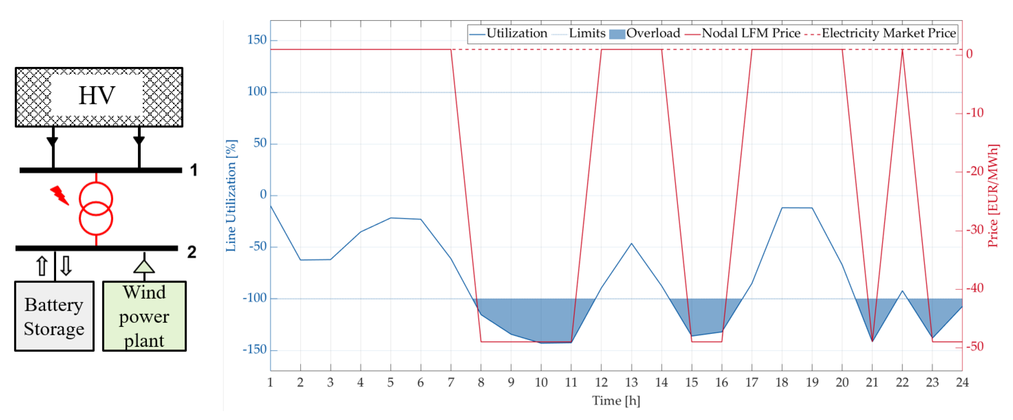
6.1. 2-Node Demonstration System

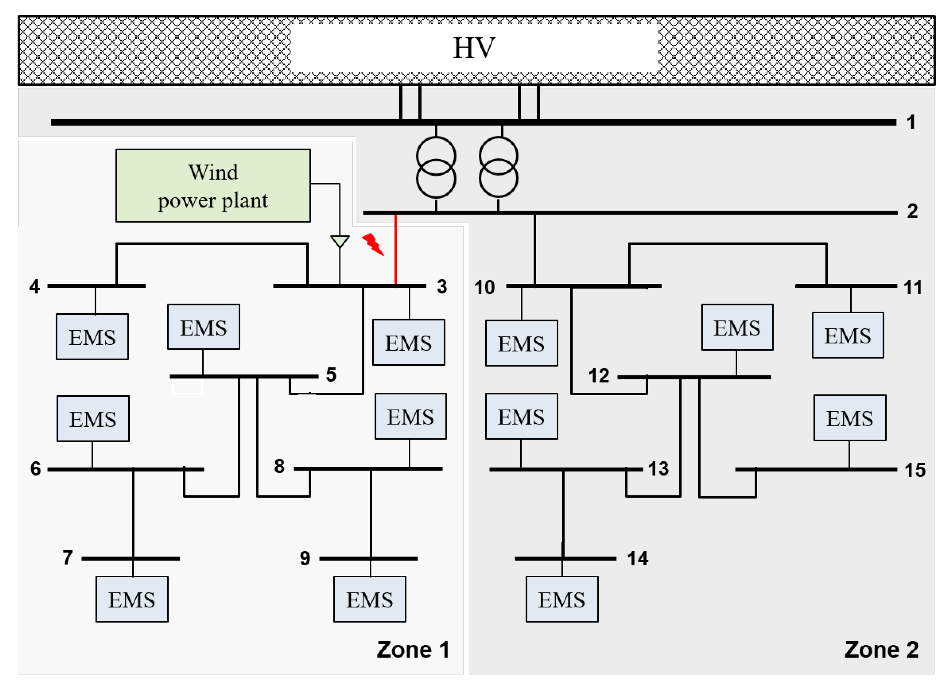
The two-node demonstration system in consideration comprises a WPP with a capacity of 14.3 MW and a BSS with a capacity of 0.76 MW/ 0.96 MWh at the same station as well as a connecting transformer to the transmission system. The BSS is fully discharged (SOC = 0 MWh) in the beginning. The grid structure of the case study is shown in the left part of Figure 9. For our case study, we assume that the connecting transformer has a thermal limit of 10 MW. The transformer is overloaded by the wind feed-in, leading to a cyclical overload as depicted in Figure 9. The overload shown here is based on the electricity market schedule without LFMs as this congestion forecast is the basis of inc-dec-gaming strategies without the consideration of market power. The shown utilization of the transformer only results from the WPP feed-in time series. To solve the congestion, the SO has to curtail the WPP. We assume curtailment penalty costs of 50 EUR/MWh and, for simplicity, that the prices of electricity (day-ahead and intraday) are constant (at 1 EUR/MWh). The considered penalty costs reflect additional lost revenues based on feed-in tariffs for the WPP operator. The constant electricity price ensures that electricity market participation yields no earning opportunity, i.e., is not carried out without inc-dec-gaming. Due to the cost of curtailment, the nodal prices at node two are equal to $-49$ EUR/MWh in congestion times and equal to the electricity price in all other time steps.

It can further be observed that theoretically, the BSS operator could create an additional congestion in time step 7. However, this requires market power (that we do not consider in the model to focus solely on inc-dec-gaming, c.f. Section 5). Thus, the BSS market behavior presented here can be viewed as the behavior of several small operators that do not have the capacity to create additional congestions. Without the ability to produce new congestions, such small operators only bid in pre-determined congestion times in the LFM. Their market behavior would be equal, therefore the BSS considered here is viewed as an aggregation of several small BSS.

The market schedules of the different operational planning approaches for the BSS are shown in Figure 10. Note that in the figures of this section, positive power is defined as consumption and negative power is defined as generation. The $DayAhead$ bars represent the electricity market schedule. As the intrady price is assumed to be equal to the day-ahead price, the schedule can already be determined day-ahead. The $LF{M}_{Flex}$ and $LF{M}_{Comp}$ bars describe the flexibility and compensation offers. When evaluating the schedules for the different operational planning approaches, first of all we can see from the SeqOpt results, that without LFMs, the BSS would not participate in the electricity market (due to the constant electricity price). Therefore, the $DayAhead$ schedules are equal to zero in that case. In the SeqOpt operational planning, all flexibility is offered in the LFM for CM.

The SeqOpt results give an indication of flexibility offers without gaming. It can be seen that due to the technical restrictions of the BSS, i.e., the limited SOC capacity, the BSS is not able to offer flexibility in all time steps with congestions. While the transformer is overloaded from hours 8 to 11, flexibility is only offered in two of the four time steps. This further shows that when not taking the time-coupling constraints into account and only considering single time steps individually, DER flexibility for LFM participation can be overestimated.

Additionally, it can be seen how the compensation is used in times with no congestion to regain flexibility potentials and thus offer further flexibility in later points of time. Thus, with compensation the BSS is able to provide more flexibility for CM.

In contrast to the SeqOpt approach, when the BSS operator anticipates the LFM prices (RA-SimultOpt and RN-SimultOpt), the operator participates in the electricity market. Since no earning opportunities exist in the electricity market (due to the constant electricity price), we can derive that electricity market participation in our example is only carried out to increase the operator’s flexibility offer, i.e., inc-dec-gaming. For example, this can be observed in the RN-SimultOpt results in all time steps with congestions. (The electricity market and LFM offers the BSS in the RN-SimultOpt results exceed the technical capacity of the BSS as the BSS operator anticipates that the LFM activation and the electricity market offer cancel each other out. We have limited the maximum offering at twice the capacity as the optimization problem will maximize the inc-dec-capacity (when not considering the non-activation)).

There, the operator is offering generation in the electricity market and additional demand flexibility in the LFM. Since the SO has a demand for additional demand flexibility, the flexibility offers will be accepted. Thus, the electricity market and LFM offers cancel each other out and do not change the transformer power flow, as can be seen by looking at the “total” market schedule in Figure 10. Nonetheless, the BSS operator buys electricity in the LFM to sell it in the electricity market due to the additional earnings enabled by the price spread.

For the RA-SimultOpt results, some parallels in market behavior can be seen: In time steps 10, 15, 21, and 24, the BSS operator offers generation and load demand, i.e., uses inc-dec-gaming to increase its profits. However, we can identify significant differences compared to the RN-SimultOpt schedules. The RA-SimultOpt modeling that ensures technical feasibility for all LFM activation levels reduces the inc-dec-volumes. The operator has only in some of the congestion time steps the ability to offer opposite schedules in both markets. Additionally, the amounts offered are smaller because they are limited by the technical BSS capacity of 0.76 MW. Therefore, the total inc-dec-gaming amount is limited by the risk-averse modeling. Furthermore, in order to offer BSS generation, the operator has to buy electricity in time step 7. The additional energy bought in the LFM is compensated between congestion times to regain flexibility potentials, as with the SeqOpt approach.

Based on the comparison of operational planning results we conclude that the anticipation of LFM prices and flexibility demands leads to inc-dec-gaming. However, the detailed modeling of technical constraints and the modeling of no short-selling significantly reduces the total inc-dec-volume. It is therefore key to consider a high level of modeling detail when analyzing inc-dec-gaming in LFMs.

To demonstrate the effect of short-selling on the technical constraints of the BSS, we evaluate the SOC in the RN-SimultOpt and RA-SimultOpt schedules for a non-activation of LFM bids. The BSS SOC limits and the resulting SOCs are shown in Figure 11. The SOCs are evaluated by taking the cumulated sum of the electricity market schedules for the case of non-activation and by evaluating the SOC results of the operational planning for the case of activation.

We see that for the RA-SimultOpt SOC, in both cases the limits of the BSS are not violated, i.e., the technical schedule remains feasible for all levels of activation. In contrast, the RN-SimultOpt SOC is only feasible when considering the activation of LFM bids. If the LFM bids are not activated, the BSS operator is selling energy that it cannot provide because its BSS is not charged. The theoretical SOC is decreasing, thus violating the SOC constraints. Therefore, if the LFM bids do not get activated, the BSS operator will violate its original electricity market schedule. It cannot sell electricity in all of the time steps (because the buying was planned to happen in the LFM); therefore, the BSS operator either does not fulfill the electricity market schedule or it has to re-buy electricity in the intraday market. When the electricity market schedule is communicated to the SO as the baseline of asset operation (and considered by the SO for the congestion forecast), this deviation from the original baseline enables the detection of inc-dec-gaming by the SO.

In Appendix A, a more detailed discussion of the bid structure and its connection to the BSS technical constraints is provided.

6.2. 15-Node System

For the exemplary case study, a 15-node medium-voltage grid is considered as depicted in Figure 12. It has a radial grid topology with a transformer at node 1 that connects the test system with the overlaying high-voltage grid. The individual branches are either cables or over-headlines parameterized using typical technical parameters. The thermal line limits range from 5–7 MW. Different DERs can be found throughout the grid, operated and aggregated at the individual nodes by individual EMSs. The installed capacities of the technologies can be found in the Appendix B and have been dimensioned based on a synthetic medium-voltage Simbench grid [46]. The technology portfolio contains household and commercial loads, PVs, a WPP, BSSs, EVs, CHPs as well as P2H systems. The proportions between the installed technology capacities are based on the scenario framework for the German Network Development Plan [47]. The normalized time series (electrical and heat demand, WPP and PV generation) of the case study are derived from [48] and scaled to the installed capacities. It should be noted that the system is especially dominated by the large wind power plant at node 2 resulting in frequent congestion on the line between node 2 and 3 as depicted in Figure 12. Due to the congestion on the line from node 2 to node 3, the grid area is split into two different zones in times of congestion: In zone 1, the WPP has to be curtailed, therefore resulting in a demand for additional load to prevent curtailment. In contrast, no restrictions exist in zone 2.

We use a typical, exemplary electricity price time series with price peaks in the morning and in the evening (cf. Figure 13). In addition, we assume an offset of 1 EUR/MWh in the LFM price offers of the EMS, whenever nodal prices of the flexibility market converge to the electricity prices. This ensures that the market participants have an incentive to bid within the flexibility market (as otherwise the EMS operators would see no earning opportunity in the LFM, c.f. Section 5). Cost of curtailment are assumed to be 50 EUR/MWh, as in the 2-node case.

As the status quo CM (without LFM, i.e., no CM contribution of EMSs) is carried out, several congestion times are identified as shown in Figure 13. (As in Figure 9, the overload shown here is based on the electricity market schedule without LFMs as this congestion forecast is the basis of inc-dec-gaming strategies without the consideration of market power.)

Due to the flexibility potential in the grid, the benchmark calculation with all flexibility considered at marginal cost (and full control by the DSO) shows that the load-based flexibility can be used to solve the congestion without curtailment in all but one hour (time step 23). Therefore, these flexibility prices (as approximations of competitive LFM prices) converge to the electricity prices as depicted in Figure 13. Due to the minimum price offset, the anticipated (and offered) LFM prices are slightly lower than the electricity price in time steps with price convergence. These LFM prices are used as the price expectation of the EMS operational planning.

In Figure 14, Figure 15 and Figure 16, the technology and market schedules for the operational planning of the EMS located at node 3 are shown exemplary to demonstrate the different market behavior of the EMSs in zone 1. The EMS is an aggregation of all electrical load, BSSs and P2H systems at node 3. We identify similar effects as in the 2-node case study:

Compensation is used to regain flexibility potentials and to increase flexibility offers. Furthermore, the amount of inc-dec-gaming is significantly higher in the RN-SimultOpt mode than in the RA-SimultOpt mode due to the technical limitations. Note that the inc-dec-gaming of RA-SimultOpt is not expressed as opposite bids in the LFM and in the electricity market but can only be detected by comparing the electricity market schedule of RA-SimultOpt with the SeqOpt market schedule. Without anticipation of the LFM prices, the EMS operator would bid the optimal electricity market schedule (SeqOpt). Without any activation in the LFM, the electricity market schedule of SeqOpt has higher earnings or lower cost than the RA-SimultOpt schedule. Inc-dec-gaming is only a reduction of load in the electricity market compared to the "true" electricity market schedule because in the RA-SimultOpt approach the electricity market schedule has to ensure a feasible supply of the load and DERs without any activation of LFM bids.

The flexibility offers in our case study for the SeqOpt mode are relatively low. This can be explained with the LFM prices. The electricity market and LFM prices only differ slightly in congestion times (cf. Figure 13), leading to relatively low earning opportunities. Since flexibility is limited and can only increased, the cost for compensation also needs to be taken into account. Considering the cost of compensation, flexibility is only offered if the price for buying energy in the LFM is lower than the price for compensation in later time steps, thus leading to reduced flexibility offerings.

The quantitative results for the case study are presented in

Table 1. Quantitative results of case study.

CM Case	Status Quo	Benchmark (all Flexibility at Marginal Cost)	SeqOpt	RA-SimultOpt	RN-SimultOpt
CM costs [EUR]	878.96	37.06	813.69	870.71	1460.8
Total Overload [MWh]	12.55	12.55	12.55	19.71	99.27
Curtailment volume [MWh]	12.55	0.11	9.06	6.70	11.78
Offered Flexibility [MWh] (% activation)	-	-	3.49 (100%)	13.4 (95%)	87.49 (100%)
Offered Compensation [MWh] (% activation)	-	-	0.93 (100%)	7.76 (92%)	6.74 (100%)

. The considered evaluation parameters are CM costs, total overload of the line between nodes 2 and 3, the curtailed energy, the offered flexibility and the offered compensation.

The CM costs are defined as the sum of cost of curtailment, cost (or earnings) of accepted LFM bids, cost (or earnings) of accepted compensation, and the cost (or earnings) of balancing energy. The LFM bids and compensation can be either cost or earnings, depending on the direction of flexibility, e.g., if a EMS operator offers additional load and a positive price, the SO gets paid by the EMS operator for an activation of that flexibility bid. Furthermore, for compensation measures, the activation cost of compensation and balancing energy cancel each other out since they are assumed to be priced equally in our case study.

The overload on the line is defined as the congestion volume based on the electricity market schedules. Thus, the overload changes depending on the considered operational planning approach due to inc-dec-gaming. It is therefore an indicator on inc-dec-volumes.

The curtailment volume measures the total curtailment necessary in CM. The offered flexibility is defined as the sum of LFM flexibility bids, whereas the offered compensation is defined as the sum of the offered compensation contained in the LFM bids.

As expected, the CM costs are lowest for the theoretical benchmark. Furthermore, the cost in the SeqOpt case are lower than for the status quo as additional (and cheaper) flexibility is offered to the SO to solve the same congestion volume. In contrast to the SeqOpt mode, the congestion volume increases for RA-SimultOpt and RN-SimultOpt due to inc-dec-gaming.

While the congestion volume only increases moderately from 12.55 MWh to 19.71 MWh with RA-SimultOpt, it increases by a factor of more than 8 with RN-SimultOpt. This steep increase can already be observed when comparing the schedules in Figure 16. Accordingly, the cost for CM are increased in the RN-SimultOpt mode compared to the status quo without LFMs.

In contrast, even with an increased CM volume in the RA-SimultOpt mode, the CM costs are lower than for the status quo without LFMs. This can be explained by the LFM price effect: Due to competition, the LFM prices are close to the balancing prices (which are equal to the electricity market price in our case study) as explained in Section 5. Instead of having to pay 50 EUR/MWh for curtailment, the SO can sell energy to the DER EMS (while the cost for balancing do not change). Thus, even with a higher CM volume, the CM cost decrease. Nonetheless, the minimum CM costs of the benchmark are not reached.

The curtailment volume for the SeqOpt case is higher than the RA-SimultOpt case due to the lower amount of flexibility offered. The lower flexibility offer can be explained by the independent determination of electricity market schedules. With the fixed schedules of SeqOpt, less flexibility can be offered in the LFM. In contrast, as the electricity market schedule and the LFM bids are determined simultaneously in the RA-SimultOpt mode, through a changed electricity market schedule (also in non-congestion time steps) the EMS operator is able to increase its amount of flexibility offered in the LFM. This extra amount offered (compared to SeqOpt) exceeds the amount used for inc-dec-gaming, resulting in a net extra flexibility of 2.36 MWh. Furthermore, it has to be noted, due to the convergence of LFM prices to electricity prices, that the DER EMS (in all modes) have a limited incentive to offer all potential flexibility in the LFM. Within the framework, each EMS optimizes its own earnings, thus only offering flexibility such that earnings are maximized. Therefore, the theoretical cost and curtailment optimum of the benchmark is not reached with the LFM for any of the modes.

The acceptance ratios for the RN-SimultOpt show that all LFM bids are accepted as this is the cost-minimum solution for the CM. In that case, inc-dec-gaming would not be detected by a deviation from the electricity market schedule baseline. However, if the SO added a random non-activation of bids [36], inc-dec-gaming can be detected. Therefore, it is reasonable that the EMS operators would act risk-averse in reality and offer only technically feasible schedules as in the RA-SimultOpt mode.

The case study presented here shows how the assumptions on operational planning modeling influence the evaluation of CM costs when considering LFMs. If we consider no short-selling of flexibility by the DER operators, the inc-dec-gaming potential is decreased. Furthermore, we have observed how the time-coupling constraints of storage systems limit the gaming potentials of DERs in LFMs. Therefore, a detailed modeling of technical constraints is needed when evaluating LFM participation.

The aim of this case study is to demonstrate the modeling approach presented in this paper and not to evaluate the advantages of LFMs. We have shown how the modeling assumptions influence inc-dec-gaming potentials and thus the cost of CM. The question of how big the problem of inc-dec-gaming is in reality needs to be further evaluated with a broad range of case studies. For example, a congestion in a single time step with low competition will still lead to increased CM cost in our modeling (as argued in [31]) because the flexibility for gaming is less limited and low risk can be assumed.

However, the results of RA-SimultOpt and SeqOpt present the extreme cases (behavior with full and with no anticipation of LFMs) of operational planning that is to be expected in LFMs without uncertainties since the RN-SimultOpt approach poses the risk of electricity market schedule deviations due to non-activation of LFM bids. Therefore, these limit cases can be used to easily determine the limit outcomes of LFM participation as real market behavior will be expected to be a something in-between these outcomes.

The results show that with RA-SimultOpt, inc-dec-gaming is still possible. Therefore, further anti-inc-dec-measures such as market monitoring are still necessary for LFM implementations in reality. This paper does not take into account any inc-dec-measures. However, the framework presented in this paper can be used as an evaluation method for proposed anti-inc-dec-measures and market monitoring [32].

We have abstracted from uncertainties in this paper to examine fundamental factors of LFM participation. With uncertainties of prices, congestions, and activation of LFM bids, the LFM participation in reality is expected to be less inclined to inc-dec-gaming. As uncertainties grow, the trade-off between potential earnings and the potential losses (and penalties) of inc-dec-gaming becomes riskier, thus decreasing the incentive for inc-dec-gaming.

7. Conclusions and Outlook

The ongoing decentralization of the European energy system leads to new requirements for grid CM. To integrate load-based, distributed flexibility into CM, LFMs are proposed as a market-based solution.

However, the flexibility potential for LFM participation is limited by the time-coupling constraints of storage systems. Therefore, we present a time-coupled formulation for LFM bids to take the time-coupled structure into account and to increase the flexibility of LFM bids.

Another key issue for LFM evaluation is the potential of inc-dec-gaming. Therefore, we provide a framework to determine the risk-averse gaming potential of DERs in a deterministic setting.

The presented case studies show the effectiveness of the LFM bidding formulation to increase the flexibility offered in LFMs. Additionally, we show how the detailed modeling of asset constraints and market participation influences the LFM and CM.

The modeling approach presented here can be used as the basis for an assessment of LFMs and the impact of operational planning of DER EMS on electricity markets and congestions. Furthermore, it can be the basis for further investigations on LFM participation. The expansion to consider uncertainties (e.g., electricity market prices, congestion times and volumes, LFM prices) can be used to provide a broader view on the market opportunities and risks of DER operators. The issue of market-power can be addressed by an expansion of the model with game-theoretic approaches. Several anti-inc-dec-gaming measures are currently discussed and could further be evaluated with our framework. Additionally, only active power is considered in this paper. Therefore, in future work reactive power and voltage limit violations can be considered within LFMs.

The case studies presented here are only small systems with a limited number of nodes. The framework presented in this paper consists of the independently solvable models for DER EMS operational planning, CM and LFM clearing. Only the CM incorporating all flexibility at marginal costs takes into account the different models simultaneously to calculate the competitive LFM clearing prices. To improve scale-ability to a high number of grid nodes and DER EMS models, this optimization problem can be decomposed and the DER EMS operational planning as well as the LFM clearing can be solved iteratively to determine the converging LFM prices.

Within the ongoing research project, “magical”, the developed bid structure and operational planning approach will be applied to LFMs for transmission system CM to examine the interactions between LFMs, the European wholesale electricity market and CM.

References

1. Consentec. Quantitative Analysen zu Beschaffungskonzepten für Redispatch. In Sammlung Verschiedener Berichte und Kurzpapiere aus dem Vorhaben “Untersuchung zur Beschaffung von Redispatch” (Projekt 055/17) im Auftrag des Bundesministeriums für Wirtschaft und Energie. 2019. Available online: https://www.bmwi.de/Redaktion/DE/Publikationen/Studien/untersuchung-zur-beschaffung-von-redispatch.pdf (accessed on 20 May 2021).
2. BDEW, “Redispatch in Deutschland: Auswertung der Transparenzdaten April 2013 bis Einschließlich September 2020”, Berlin. November 2020. Available online: https://www.bdew.de/media/documents/2020_Q3_Bericht_Redispatch_GOQPsvY.pdf (accessed on 25 February 2021).
3. Nodes, E-Bridge, Pöyry, “Marktbasiertes Engpassmanagement als Notwendige Ergänzung zum Regulierten Redispatch in Deutschland”. 2019. Available online: https://www.e-bridge.de/wp-content/uploads/2019/09/20190904_NODES_Marktbasierter_RD_DEUTSCH_v10_sent.pdf (accessed on 30 March 2021).
4. Ramos, A.; De Jonghe, C.; Gómez, V.; Belmans, R. Realizing the smart grid’s potential: Defining local markets for flexibility. Util. Policy 2016, 40, 26–35. [Google Scholar] [CrossRef]
5. European Commission. Clean Energy Package: Ensure Wholesale-Retail Integration; Electricity Directive Article; European Commission: Luxembourg, 2019; p. 32. [Google Scholar]
6. Jin, X.; Wu, Q.; Jia, H. Local flexibility markets: Literature review on concepts, models and clearing methods. Appl. Energy 2020, 40, 114387. [Google Scholar] [CrossRef] [Green Version]
7. Buchmann, M. How decentralization drives a change of the institutional framework on the distribution grid level in the electricity sector—The case of local congestion markets. Energy Policy 2020, 145, 111725. [Google Scholar] [CrossRef]
8. Radecke, J.; Hefele, J.; Hirth, L. Markets for Local Flexibility in Distribution Networks. ZBW-Leibniz Inform. Centre Econ. 2019. Available online: http://hdl.handle.net/10419/204559 (accessed on 20 May 2021).
9. Heilmann, E.; Klempp, N.; Wetzel, H. Design of regional flexibility markets for electricity: A product classification framework for and application to German pilot projects. Util. Policy 2020, 67, 101133. [Google Scholar] [CrossRef]
10. Dronne, T.; Roques, F.; Saguan, M. Local Flexibility Markets for Distribution Network Congestion-Management: Which Design for Which Needs? Chaire European Electricity Markets/Working Paper #47. December 2020. Available online: http://www.ceem-dauphine.org/working/en/LOCAL-FLEXIBILITY-MARKETS-FOR-DISTRIBUTION-NETWORK-CONGESTION-MANAGEMENT-WHICH-DESIGN-FOR-WHICH-NEEDS (accessed on 20 May 2021).
11. Anaya, K.L.; Pollitt, M.G. Milestone 1: A Review of International Experience in the use of Smart Electricity Platformes for the Procurement of Flexibility Services (Part 1). Merlin Project Report. 2020. Available online: https://project-merlin.co.uk/wp-content/uploads/2020/05/SSEN_Cambridge_V5b_pages.pdf (accessed on 20 May 2021).
12. Schittekatte, T.; Meeus, L. Flexibility markets: Q&A with project pioneers. Util. Policy 2020, 63, 101017. [Google Scholar] [CrossRef] [Green Version]
13. ENERA Consortium. Using Enera’s Experience to Complement the Upcoming Redispatch Regime with Flexibility from Load & Other Non-Regulated Assets. 2020. Available online: https://projekt-enera.de/wp-content/uploads/enera-Improving-redispatch-thanks-to-flexibility-platform-experience.pdf (accessed on 20 May 2021).
14. Correa-Florez, C.A.; Michiorri, A.; Kariniotakis, G. Optimal Participation of Residential Aggregators in Energy and Local Flexibility Markets. IEEE Trans. Smart Grid 2020, 11, 1644–1656. [Google Scholar] [CrossRef]
15. Esmat, A.; Usaola, J.; Moreno, M.A. Distribution-level flexibility market for congestion management. Energies 2018, 11, 1056. [Google Scholar] [CrossRef] [Green Version]
16. Olivella-Rosell, P.; Lloret-Gallego, P.; Munné-Collado, Í.; Villafafila-Robles, R.; Sumper, A.; Ottessen, S.Ø.; Rajasekharan, J.; Bremdal, B.A. Local Flexibility Market Design for Aggregators Providing Multiple Flexibility Services at Distribution Network Level. Energies 2018, 11, 822. [Google Scholar] [CrossRef] [Green Version]
17. Torbaghan, S.S.; Blaauwbroek, N.; Kuiken, D.; Gibescu, M.; Hajighasemi, M.; Nguyen, P.; Smit, G.J. M; Roggenkamp, M.; Hurink, J. A market-based framework for demand side flexibility scheduling and dispatching. Sustain. Energy Grids Netw. 2018, 14, 47–61. [Google Scholar] [CrossRef] [Green Version]
18. Zhang, C.; Ding, Y.; Nordentoft, N.C.; Pinson, P.; Østergaard, J. FLECH: A Danish market solution for DSO congestion management through DER flexibility services. J. Mod. Power Syst. Clean Energy 2014, 2, 126–133. [Google Scholar] [CrossRef] [Green Version]
19. Kulms, T.; Meinerzhagen, A.; Koopmann, S.; Schnettler, A. Development of an agent-based model for assessing the market and grid oriented operation of distributed energy resources. Energy Procedia 2017, 135, 294–303. [Google Scholar] [CrossRef]
20. Coninx, K.; Deconinck, G.; Holvoet, T. Who gets my flex? An evolutionary game theory analysis of flexibility market dynamics. Appl. Energy 2018, 218, 104–113. [Google Scholar] [CrossRef]
21. Li, R.; Wu, Q.; Oren, S.S. Distribution locational marginal pricing for optimal electric vehicle charging management. IEEE Trans. Power Syst. 2013, 29, 203–211. [Google Scholar] [CrossRef] [Green Version]
22. Olivella-Rosell, P.; Bullich-Massagué, E.; Aragüés-Peñalba, M.; Sumper, A.; Ottesen, S.Ø.; Vidal-Clos, J.A.; Villafáfila-Robles, R. Optimization problem for meeting distribution system operator requests in local flexibility markets with distributed energy resources. Appl. Energy 2018, 210, 881–895. [Google Scholar] [CrossRef]
23. Brunekreeft, G.; Buchmann, M.; Höckner, J.; Palovic, M.; Voswinkel, S.; Weber, C. Thesenpapier: Ökonomische und regulatorische Fragestellungen zum enera-FlexMarkt. In EWL Working Papers; University of Duisburg-Essen, Chair for Management Science and Energy Economics: Essen, Germany; Bremen, Germany, 2020. [Google Scholar]
24. Meißner, A.C.; Dreher, A.; Knorr, K.; Vogt, M.; Zarif, H.; Jürgens, L.; Grasenack, M. A co-simulation of flexibility market based congestion management in Northern Germany. In Proceedings of the 16th International Conference on the European Energy Market (EEM), Ljubljana, Slovenia, 18–20 September 2019. [Google Scholar]
25. Schmitt, C.; Sous, T.; Blank, A.; Gaumnitz, F.; Moser, A. A Linear Programing Formulation of Time-Coupled Flexibility Market Bids by Storage Systems. In Proceedings of the 2020 55th International Universities Power Engineering Conference (UPEC), Torino, Italy, 1–4 September 2020; pp. 1–6. [Google Scholar] [CrossRef]
26. Schweppe, F.C.; Caramanis, M.C.; Tabors, R.D.; Bohn, R.E. Spot Pricing of Electricity; Springer Science & Business Media: Boston, MA, USA, 1988. [Google Scholar]
27. Franco, J.F.; Rider, M.J.; Lavorato, M.; Romero, R. A mixed-integer LP model for the reconfiguration of radial electric distribution systems considering distributed generation. Electr. Power Syst. Res. 2013, 97, 51–60. [Google Scholar] [CrossRef]
28. Franken, M.S.; Barrios, H.; Schrief, A.B.; Moser, A. Transmission expansion planning via power flow controlling technologies. IET Gener. Transm. Distrib. 2020, 14, 3530–3538. [Google Scholar] [CrossRef]
29. Linnemann, C.; Echternacht, D.; Breuer, C.; Moser, A. Modeling optimal redispatch for the european transmission grid. In Proceedings of the 2011 IEEE Trondheim PowerTech, Trondheim, Norway, 19–23 June 2011. [Google Scholar]
30. Schermeyer, H.; Vergara, C.; Fichtner, W. Renewable energy curtailment: A case study on today’s and tomorrow’s congestion management. Energy Policy 2018, 112, 427–436. [Google Scholar] [CrossRef]
31. Hirth, L.; Schlecht, I. Redispatch Markets in Zonal Electricity Markets: Inc-Dec Gaming as a Consequence of Inconsistent Power Market Design (Not Market Power). 2019. Available online: http://hdl.handle.net/10419/194292 (accessed on 20 May 2021).
32. Cramton, P. Local Flexibility Market. University of Cologne and University of Maryland Working Paper. 2019. Available online: www.cramton.umd.edu/papers2015-2019/cramton-local-flexibility-market.pdf (accessed on 20 May 2021).
33. Hogan, W. Restructuring the Electricity Market: Institutions for Network Systems; Harvard University: Cambridge, MA, USA, 1999. [Google Scholar]
34. Brunekreeft, G.; Pechan, A.; Palovic, M.; Meyer, R.; Brandstätt, C.; Buchmann, M. Kurzgutachten zum Thema ‘Risiken Durch Strategisches Verhalten von Lasten auf Flexibilitäts- und anderen Energiemärkten’; Report; Deutsche Energie-Agentur (dena): Bremen, Germany, 2020. [Google Scholar]
35. Nodes AS; DNV-GL. Market-Based Redispatch—Why It Works! 2020. Available online: https://nodesmarket.com/publications/ (accessed on 20 May 2021).
36. ENKO consortium. Scheinflexibilität–Eine beherrschbare Herausforderung für ENKO. Whitepaper. 2020. Available online: https://www.enko.energy/wp-content/uploads/ENKO-White-Paper-Scheinflexibilität.pdf (accessed on 20 May 2021).
37. Kulms, T.; Meinerzhagen, A.; Koopmann, S.; Schnettler, A. A simulation framework for assessing the market and grid driven value of flexibility options in distribution grids. J. Energy Storage 2018, 17, 203–212. [Google Scholar] [CrossRef]
38. Geschermann, K.; Moser, A. Evaluation of market-based flexibility provision for congestion management in distribution grids. In Proceedings of the 2017 IEEE Power & Energy Society General Meeting, Chicago, IL, USA, 16–20 July 2017. [Google Scholar]
39. Thie, T.; Vasconcelos, M.; Schnettler, A.; Kloibhofer, L. Influence of European Market Frameworks on Market Participation and Risk Management of Virtual Power Plants. In Proceedings of the 2018 15th International Conference on the European Energy Market (EEM), Lodz, Poland, 27–29 June 2018; pp. 1–5. [Google Scholar] [CrossRef]
40. Thie, N. Risikomanagement in der Direktvermarktung erneuerbarer Energien. Ph.D. Thesis, RWTH Aachen University, Aachen, Germany, 2020. [Google Scholar] [CrossRef]
41. Vertgewall, C.M.; Trageser, M.; Kurth, M. Modeling of Location and Time Dependent Charging Profiles of Electric Vehicles Based on Historic User Behavior. Unpublished work, 2021. [Google Scholar]
42. Gils, H.C. Economic potential for future demand response in Germany—Modelling approach and case study. Appl. Energy 2016, 162, 401–415. [Google Scholar] [CrossRef] [Green Version]
43. Carrion, M.; Arroyo, J.M. A computationally efficient mixed-integer linear formulation for the thermal unit commitment problem. IEEE Trans. Power Syst. 2006, 21, 1371–1378. [Google Scholar] [CrossRef]
44. Ventosa, M.; Baıllo, A.; Ramos, A.; Rivier, M. Electricity market modeling trends. Energy Policy 2005, 33, 897–913. [Google Scholar] [CrossRef]
45. NEMO Committee. EUPHEMIA Public Description—Single Price Coupling Algortithm. 2019. Available online: http://www.nemo-committee.eu/assets/files/190410_Euphemia%20Public%20Description%20version%20NEMO%20Committee.pdf (accessed on 20 May 2021).
46. Meinecke, S.; Sarajlić, D.; Drauz, S.R.; Klettke, A.; Lauven, L.-P.; Rehtanz, C.; Moser, A.; Braun, M. SimBench—A Benchmark Dataset of Electric Power Systems to Compare Innovative Solutions Based on Power Flow Analysis. Energies 2020, 13, 3290. [Google Scholar] [CrossRef]
47. Bundesnetzagentur für Elektrizität, Gas, Telekommunikation, Post und Eisenbahnen (BNetzA). Genehmigung des Szenariorahmens 2019–2030. 2018. Available online: https://www.netzentwicklungsplan.de/sites/default/files/paragraphs-files/Szenariorahmen_2019-2030_Genehmigung_0_0.pdf (accessed on 30 March 2021).
48. Müller, C.; Hoffrichter, A.; Wyrwoll, L.; Schmitt, C.; Trageser, M.; Kulms, T.; Beulertz, D.; Metzger, M.; Duckheim, M.; Huber, M.; et al. Modeling framework for planning and operation of multi-modal energy systems in the case of Germany. Appl. Energy 2019, 250, 1132–1146. [Google Scholar] [CrossRef]
Figure 1. Development of CM volumes in Germany in Gigawatt hours (GWh) [2].
Energies 14 03012 g001
Figure 2. CM approach (left) and LFM time frame with sequential market participation (right).
Energies 14 03012 g002
Figure 3. Available flexibility of storage systems (based on either positive or negative activation) with and without compensation [25].
Energies 14 03012 g003
Figure 4. Anticipatory operational planning in electricity markets and LFMs with potential schedules of (a) risk-neglecting and (b) risk-averse operational planning.
Energies 14 03012 g004
Figure 5. Energy Management System (EMS) model consisting of several DERs.
Energies 14 03012 g005
Figure 6. Scenario coupling for risk-averse operational planning.
Energies 14 03012 g006
Figure 7. Overview on cases of operational planning.
Energies 14 03012 g007
Figure 8. Overview on model interconnections in modeling framework.
Energies 14 03012 g008
Figure 9. 2–node case study: structure, overloads and congestion prices.
Energies 14 03012 g009
Figure 10. Market schedules of BSS for the three different operational planning modes (Congestion times shaded in grey).
Energies 14 03012 g010
Figure 11. Comparison of theoretical SOCs when considering all flexibility activation S O C a l l and only considering electricity market schedules S O C o n l y E M .
Energies 14 03012 g011
Figure 12. Grid structure of case study.
Energies 14 03012 g012
Figure 13. Utilization of line between nodes 2 and 3 and electricity price as well as nodal congestion prices in zone 1.
Energies 14 03012 g013
Figure 14. Schedules of operational planning SeqOopt of EMS at node 3 (Congestion times shaded in grey).
Energies 14 03012 g014
Figure 15. Schedules of operational planning RA-Simultopt of EMS at node 3 (Congestion times shaded in grey).
Energies 14 03012 g015
Figure 16. Schedules of operational planning RN-Simultopt of EMS at node 3 (Congestion times shaded in grey).
Energies 14 03012 g016