Technical and Economic Analysis of the Supercritical Combined Gas-Steam Cycle

Abstract

Combined cycle power plants are characterized by high efficiency, now exceeding 60%. The record-breaking power plant listed in the Guinness Book of World Records is the Nishi-Nagoya power plant commissioned in March 2018, located in Japan, and reaching the gross efficiency of 63.08%. Research and development centers, energy companies, and scientific institutions are taking various actions to increase this efficiency. Both the gas turbine and the steam turbine of the combined cycle are modified. The main objective of this paper is to improve the gas-steam cycle efficiency and to reach the efficiency that is higher than in the record-breaking Nishi-Nagoya power plant. To do so, a number of numerical calculations were performed for the cycle design similar to the one used in the Nishi-Nagoya power plant. The paper assumes the use of the same gas turbines as in the reference power plant. The process of recovering heat from exhaust gases had to be organized so that the highest capacity and efficiency were achieved. The analyses focused on the selection of parameters and the modification of the cycle design in the steam part area in order to increase overall efficiency. As part of the calculations, the appropriate selection of the most favorable thermodynamic parameters of the steam at the inlet to the high-pressure (HP) part of the turbine (supercritical pressure) allowed the authors to obtain the efficiency and the capacity of 64.45% and about 1.214 GW respectively compared to the reference values of 63.08% and 1.19 GW. The authors believe that efficiency can be improved further. One of the methods to do so is to continue increasing the high-pressure steam temperature because it is the first part of the generator into which exhaust gases enter. The economic analysis revealed that the difference between the annual revenue from the sale of electricity and the annual fuel cost is considerably higher for power plants set to supercritical parameters, reaching approx. USD 14 million per annum. It is proposed that investments in adapting components of the steam part to supercritical parameters may be balanced out by a higher profit.

1. Introduction

In recent years, electricity generation and conversion issues have been in the spotlight of many scientific institutions, research and development centers, energy companies, and even state governments. In the European Union as well as outside it, particular emphasis is placed on improving the efficiency of electricity generation [1,2]. Currently, high-efficiency steam turbines set to supercritical and ultra-supercritical parameters are preferred in conventional energy systems [3,4]; unfortunately, this is a coal technology.

Another marked tendency is to build combined gas-steam cycles, which allow very high efficiencies, reaching 60%, to be achieved [5]. In addition to commercial activities, various research on gas turbines with an external combustion chamber is being conducted, also allowing the electricity generation efficiency to be improved [6,7]. On the other hand, another strong and applied tendency is distributed energy [8,9], which uses renewable energy sources [10,11]. Electricity generation using more gaseous fuels from biomass gasification or biomass itself is also under analysis [12,13]. Power plants that use gas microturbines and closed cycles [14], and polygeneration [15] are developing fast. It seems that the use of the microturbines technology in distributed energy will also be developed [16,17]. This technology has seen considerable improvements in terms of efficiency and applicability due to the use of generators based on rare-earth magnets [18,19]. Research on improvements to efficiency and durability and lower building costs of energy systems based on fuel cells [20,21] or PV cells [22,23] is underway. The construction of power plants and heat and power plants using organic Rankine cycles (ORCs) [24] is a separate direction for energy development. Due to their very low temperature, ORC plants have a low efficiency of approx. 10%, only exceptionally being able to reach approx. 20% [25]. It is possible to improve the cycle efficiency by increasing the upper temperature and modifying the plant design [26,27]. Despite very considerable developments in distributed energy and alternative energy sources, it should be concluded that high-efficiency power plants with steam turbines set to supercritical parameters, combined gas-steam cycle power plants, and nuclear power plants [28] will be developed in terms of high installed capacities.

The review above showed that researchers put a lot of effort into improving the efficiency of electricity generation, whereas the aim of this paper is to improve the efficiency of the combined gas-steam cycle—and to perform an economic evaluation of such improvement. The concept of the combined cycle power plant is to use hot exhaust gases leaving the gas turbine in order to generate steam in a heat recovery steam generator, which will be used to drive the steam turbine. Plants of this type use two thermodynamic cycles. The Brayton cycle is used in the gas turbine, while the Rankine cycle in the steam part. The gas turbine cycle is referred to as a topping cycle, while the steam part cycle as a bottoming cycle [29]. The names stem from the fact that high-temperature heat is supplied in the topping cycle, whereas heat at a much lower temperature leaves the bottoming cycle. A heat recovery steam generator (HRSG) links these two cycles. In recent years, combined cycles have moved from the concept of improving the efficiency of electricity generation systems to the most preferred fossil fuel power plants [30]. One distinctive feature of combined cycles is that power is generated from both the gas turbine and the steam turbine when burning fuel. The comparison of the volume of CO₂ emitted to the amount of energy generated is much more favorable for combined cycles than for a typical coal-fired condensing power plant [31]. Gas-steam cycles are becoming increasingly popular due to a number of advantages such as high efficiency-now exceeding 60% (the current record, 63.08%, was set in Japan in the Nishi-Nagoya power plant) [32], high operational reliability, capacity reaching 1 GW, high flexibility translating into short startup times to reach full load, process automation possibilities, and low greenhouse gas emissions [33,34].

As already mentioned, the heat recovery steam generator, based on a countercurrent heat exchanger, is what links the gas and steam cycles. The generator design includes three zones. The first one is the economizer zone in which water is heated to the saturation temperature. Then it is transferred to the evaporator zone in order to generate steam. The last zone is the superheater zone, where the temperature is increased on purpose in order to improve both the steam turbine capacity and rate of heat recovery from exhaust gases. A point at which the water evaporation process starts is crucial in the entire heat recovery process. It is the point where the temperature difference between the heat transfer exhaust gas and the receiving water must be the lowest. This difference is referred to as a pinch point. The smaller it is, the higher the efficiency of the gas-steam cycle efficiency is, but it is achieved thanks to the larger heat exchange surface—which affects the cost of the entire installation [35]. Forced circulation heat recovery steam generators are mainly used; however, there are also plants that use assisted or natural circulation heat recovery steam generators. The heat recovery process in a single-pressure HRSG is given in Figure 1, while an example of a single-pressure steam-gas combined cycle power plant is presented in Figure 2 [36]. Heat recovery steam generators must face many challenges, which include a high rate of heat recovery from exhaust gases, allowing for small pressure losses at the steam side, as well as corrosion resistance and low pressure losses at the exhaust gas side. To ensure high heat recovery efficiency and low exergy losses, the difference between the heat transfer medium and the receiving medium should be as low as possible [37]. This means that a large heat exchange surface area is required. Heat recovery steam generators that are currently designed have very low pressure losses from 25 to 30 mbar at the exhaust gas side [38]. Designs where practically any fuel is burnt in the generator are also analyzed [39,40].

A gas turbine with the highest possible efficiency should be used in order to obtain a high-efficiency gas-steam cycle. This means that new materials able to withstand higher temperatures must be used and developed. Apart from the main components such as the steam turbine, gas turbine, and the heat recovery steam generator, there have been significant developments in all systems and installations linked directly with the cycle. They all serve the same purpose—to minimize losses. At present, the following trends can be observed in order to achieve the aforementioned goals [35,39,41]:

• Higher combustion temperatures to increase gas turbine efficiency and steam cycle efficiency thanks to higher steam parameters;
• New designs for gas turbines with higher efficiencies;
• Higher gas turbine capacity to benefit from the economies of scale;
• Lower operating costs due to the use of remote control;
• Lower emissions, in particular NO₂ emissions, to reduce environmental impact;
• Better cycle loading capabilities to control partial load and frequency;
• Development of hydrogen-fueled gas turbines.

For new gas-steam cycles, an existing gas turbine model is selected and then the steam part is designed and optimized according to given requirements [42]. There are also models designed from the ground up for this type of systems. Contemporary high-capacity combined cycles use steam at a pressure up to 17 MPa, with the steam temperature at the steam turbine inlet reaching 580 °C. For steam turbines of over 100 MW, superheating is now used as standard. The trend can be expected to continue in the near future. Large power stations will operate at higher parameters, namely pressure and temperature. Before increasing steam parameters, the following issues must be analyzed [38]:

• A higher operating temperature requires the use of much more expensive alloys in the heat recovery steam generator, steam turbine, and pipelines. A higher investment cost must be justified by higher capacity and efficiency;
• A higher pressure leads to higher thickness of walls in all components, reducing thermal flexibility and increasing costs;
• A higher pressure combined with superheating reduces the main steam flow. This leads to issues with the design of high-pressure turbines.

A higher steam pressure does not necessarily mean that the efficiency of the entire combined cycle is higher. Optimization is achieved not only due to the steam cycle efficiency but also due to the extent to which exhaust gas heat is used to generate steam. The cycle efficiency will go up as the pressure increases but up to a certain point. At the same time, overall efficiency and total capacity will decrease. That is why the selection of the fresh steam pressure depends on the steam turbine efficiency, the steam cycle efficiency, and the efficiency at which heat from exhausts gases is recovered in the heat recovery steam generator.

In combined cycles, the use of multi-pressure systems (two and three-pressure heat recovery steam generators) allows to reduce the temperature difference between fluids, and thus to increase the efficiency of the entire cycle. The key task is to select the values of these pressures and divide the flow rates to obtain the highest efficiency.

As the temperature of gas turbine exhaust gases increases, the selection of an appropriate cycle configuration becomes crucial. Most frequently, a three-pressure cycle is the optimum solution for a system in which exhaust gases at a temperature of approx. 600 °C are available. A trend towards single-pressure cycles will be observed when exhaust gases at temperatures of approx. 750–800 °C start to be used.

Current combined cycle power units achieve a net efficiency of approx. 58.5% thanks to a number of improvements [38,43]. Power units currently in use are considered here. Research and tests aimed at reaching the efficiency of more than 60% are also underway. In terms of improving the efficiency of combined gas-steam cycles, three main development directions are taken: selection of optimum thermodynamic parameters in the steam part; selection of the optimum type of heat recovery steam generator; and the selection of the most favorable distribution of heated areas in the heat recovery steam generator-all with the highest cost-effectiveness of the solution in mind.

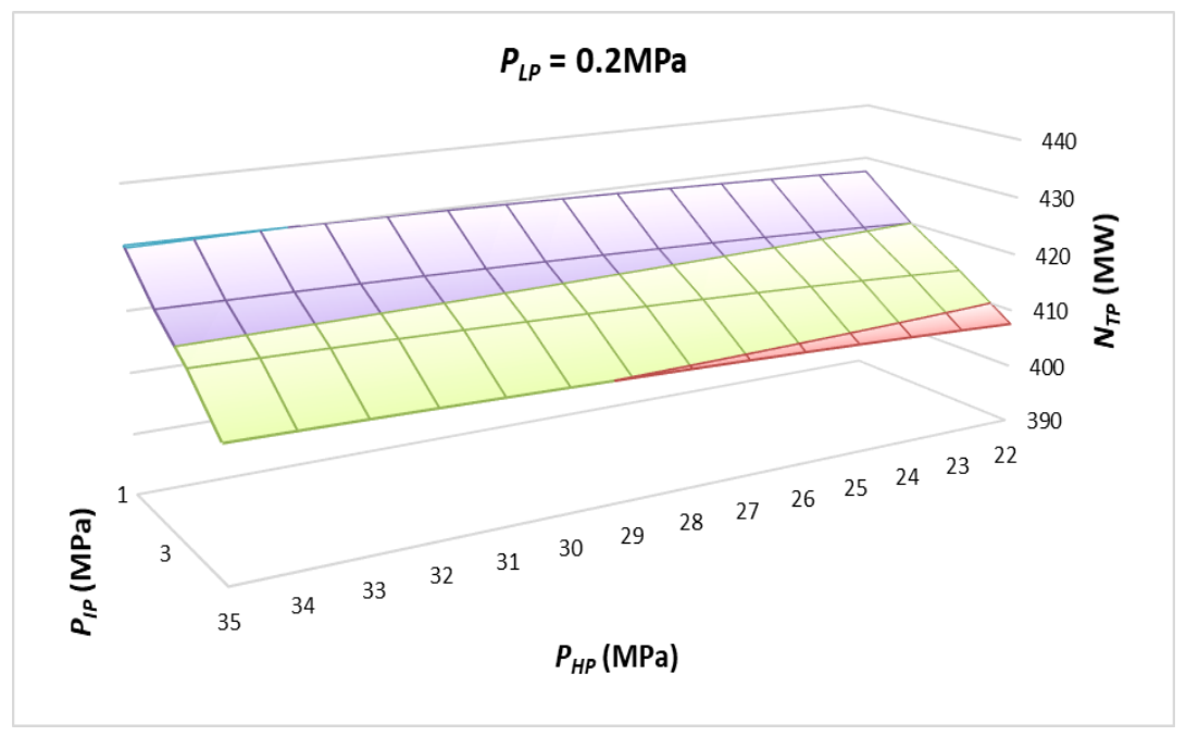
In this paper, the authors proposed using a supercritical steam pressure to improve the efficiency (Figure 3). Further on in the paper, design calculations for steam turbines were made and an economic analysis was carried out, which may form a basis for making appropriate investment and managerial decisions in terms of selecting the most optimal solution.

2. Modelling

A combined cycle power plant with the highest efficiency—the Nishi-Nagoya power plant located in Japan—was chosen as a reference power plant. Commissioned in March 2018, this power plant reaches a gross efficiency of 63.08% [32,43]. It is configured as 3 × 3 × 1. This means that the power unit includes 3 gas turbines whose exhaust gases move to 3 heat recovery steam generators. Heat is recovered from exhaust gases and steam is generated there. Then steam moves to the steam turbine. The objective of this paper is to analyze the improvement of the efficiency of this combined cycle by applying supercritical parameters in the HP part of the steam turbine. A three-pressure combined cycle power plant with superheating set to subcritical parameters (Figure 4a) and supercritical parameters (Figure 4b) was analyzed. A number of assumptions were made for the calculations and their values are presented in

Table 1. Assumed values of the efficiencies of particular cycle elements.

Description	Symbol	Value	Unit
Gas turbine capacity	NTG	280	MW
Flow rate of exhaust gases	${\dot{m}}_{exh}$	510	kg/s
Outlet temperature of exhaust gases	tG	626	°C
Superheat temperature	tG	610	°C
Mean specific heat of exhaust gases	cpexh	1.1	kJ/kg K
Pressure drop in the heat exchanger	pi/pi−1	0.01	–
Temperature increase in the deaerator	ΔtD	30	°C
Pinch point in the HRSG	ΔtHRSG	3	°C
HP turbine efficiency	ηHP	0.93	–
IP turbine efficiency	ηIP	0.94	–
LP turbine efficiency	ηLP	0.93	–
Pump efficiency	ηP	0.85	–
Mechanical efficiency	ηm	0.99	–
Leakage efficiency (losses)	ηn	0.985	–
Generator efficiency	ηG	0.98	–

[29,33,35,44].

Assuming that the pressure in the heat recovery steam generator is constant, the heat flux in exhaust gases leaving the gas turbine may be given as

$${\dot{Q}}_{GTexh}={\dot{m}}_{exh}\ast c_{pexh}\ast \Delta t={\dot{m}}_{exh}\ast c_{pexh}\ast \left(t_4^{TG}-t_1^{TG}\right) ={\dot{Q}}_{max},$$

(1)

where: ${\dot{Q}}_{max}$—heat flux in exhaust gases, ${\dot{m}}_{exh}$—exhaust gas mass flow rate, $c_{pexh}$—specific heat of exhaust gases, $t_4^{TG}$—exhaust gas temperature at gas turbine outlet, $t_1^{TG}$—temperature of exhaust gases leaving the heat recovery steam generator.

The entire steam generation process is divided into 3 stages. Heat fluxes can also be given for each of these 3 stages.

• Water heating

$${\dot{Q}}_{eco}={\dot{m}}_{med}\ast c_{pwater}\ast \Delta t={\dot{m}}_{med}\ast c_{pwater}\ast \left(t_3-t_2\right) ={\dot{Q}}_{max},$$

(2)

where: ${\dot{m}}_{med}$—mass flow rate in the steam cycle, $c_{pwater}$—specific heat of water, $t_3$—water temperature at economizer outlet, $t_2$—water temperature at economizer inlet,

• Evaporation

$${\dot{Q}}_{evo}={\dot{m}}_{med}\ast \Delta h={\dot{m}}_{TP}\ast \left(h_4-h_3\right),$$

(3)

where: $h_4$—specific enthalpy at the end of evaporation process, $h_3$—specific enthalpy in saturation point.

• Superheating

$${\dot{Q}}_{sup}={\dot{m}}_{med}\ast \Delta h={\dot{m}}_{med}\ast \left(h_5-h_4\right),$$

(4)

where: $h_5$—specific enthalpy at the end of superheating process.

The total heat flux used to generate steam is a sum of the three heat fluxes given above:

$${\dot{Q}}_{TP}={\dot{Q}}_{eco}+{\dot{Q}}_{evo}+{\dot{Q}}_{sup}.$$

(5)

Minimum temperature differences between the media that give off and receive heat are observed in two places:

• Between exhaust gases and water ($\Delta t_{exhaust-water}$);
• Between exhaust gases and steam ($\Delta t_{exhaust-steam}$).

The gas-steam cycle efficiency can be defined as [38]

$${\eta }_{GS}=\frac{N_{TG}+N_{Tp}}{{\dot{Q}}_D}={\eta }_{TG}\left(1+\frac{N_{TG}}{N_{Tp}}\right),$$

(6)

where: ${\eta }_{GS}$—gas-steam cycle efficiency, ${\eta }_{TG}$—gas turbine efficiency.

Three-pressure cycle with superheating

High pressure mass flow:

$${\dot{m}}_{HP}=\frac{{\dot{m}}_{exh}\ast c_{pexh}\ast \left(t_{exh}^{TG}-\left(t_{sat}^{HP}+∆t\right)\right)}{(h_1-h_{14})+(h_3-h_2)}.$$

(7)

Intermediate pressure mass flow:

$${\dot{m}}_{IP}=\frac{{\dot{m}}_{ehx}\ast c_{pspal}\ast \left(\left(t_{sat}^{HP}+∆t\right)-\left(t_{sat}^{IP}+∆t\right)\right)-{\dot{m}}_{HP}\ast \left(h_{14}-h_{13}\right)}{\left(h_{20}-h_{18}\right)}.$$

(8)

Low pressure mass flow:

$${\dot{m}}_{LP}=\frac{{\dot{m}}_{exh}\ast c_{pexh}\ast \left(\left(t_{nas}^{IP}+∆t\right)-\left(t_{nas}^{LP}+∆t\right)\right)-{\dot{m}}_{HP}\ast \left(h_{13}-h_{12}\right)-{\dot{m}}_{IP}\ast \left(h_{18}-h_{17}\right)}{(h_{24}-h_{22})}.$$

(9)

Outlet temperature of gas turbine fumes leaving HRSG:

$$t_{out}^{TG}= \left(t_{sat}^{LP}+∆t\right)-\frac{{\dot{m}}_{HP}\ast \left(h_{12}-h_{11}\right)+{\dot{m}}_{IP}\ast \left(h_{17}-h_{16}\right)+{\dot{m}}_{LP}\ast \left(h_{22}-h_{21}\right)}{\left({\dot{m}}_{spal}\ast C{p}_{spal}\right)}.$$

(10)

Three-pressure cycle with superheating and set to supercritical steam parameters

High-pressure steam mass flow rate:

$${\dot{m}}_{HP}=\frac{{\dot{m}}_{exh}\ast c_{pexh}\ast \left(t_{exh}^{TG}-\left(t_{13}+∆t\right)\right)}{\left(h_1-h_{13}\right)+\left(h_3-h_2\right)}.$$

(11)

Intermediate-pressure steam mass flow rate:

$${\dot{m}}_{IP}=\frac{{\dot{m}}_{exh}\ast c_{pexh}\ast \left(\left(t_{13}+∆t\right)-\left(t_{sat}^{IP}+∆t\right)\right)-{\dot{m}}_{HP}\ast \left(h_{13}-h_{12}\right)}{\left(h_{20}-h_{18}\right)}.$$

(12)

Low-pressure steam mass flow rate:

$${\dot{m}}_{LP}=\frac{{\dot{m}}_{exh}\ast c_{pexh}\ast \left(\left(t_{sat}^{IP}+∆t\right)-\left(t_{sat}^{LP}+∆t\right)\right)-{\dot{m}}_{IP}\ast \left(h_{18}-h_{17}\right)}{\left(h_{24}-h_{22}\right)}.$$

(13)

Outlet temperature of exhaust gases:

$$t_{out}^{TG}= \left(t_{sat}^{LP}+∆t\right)-\frac{{\dot{m}}_{HP}\ast \left(h_{12}-h_{11}\right)+{\dot{m}}_{IP}\ast \left(h_{17}-h_{16}\right)+{\dot{m}}_{LP}\ast \left(h_{22}-h_{21}\right)}{{\dot{m}}_{exh}\ast c_{pexh}}$$

(14)

where:

${\dot{m}}_{exh}$ mass flow rate for exhaust gases (kg/s),

${\dot{m}}_{HP}$ mass flow rate for high-pressure steam (kg/s),

${\dot{m}}_{IP}$ mass flow rate for intermediate-pressure steam (kg/s),

${\dot{m}}_{LP}$ mass flow rate for low-pressure steam (kg/s),

$h$ specific enthalpy (kJ/kg),

$c_{pexh}$ specific heat of exhaust gases (kJ/kg K),

$t_{sat}^{HP}$ high-pressure steam saturation temperature (°C),

$t_{sat}^{IP}$ intermediate-pressure steam saturation temperature (°C),

$t_{sat}^{LP}$ ow-pressure steam saturation temperature (°C),

$t_{exh}^{TG}$ exhaust gases temperature leaving gas turbine (°C),

$\Delta t$ pinch point (°C),

$t_{out}^{TG}$ temperature of exhaust gases flowing from the heat recovery steam generator (°C).

Knowing mass flow rates, it was possible to develop an initial design of steam turbine flow channels. For one-dimensional calculations of the axial turbine stage, required data include pressure at stage inlet, temperature at stage inlet, mass flow rate, isentropic enthalpy drop in the stage. These values are obtained through cycle calculations. On the other hand, thermodynamic parameters at the turbine inlet (index 0) and parameters after the isentropic transformation (index 2s) are determined based on tables containing medium properties (using REFPROP-Reference Fluid Thermodynamic and Transport Properties [45]). Other input parameters for stage calculations are assumed and then optimized if necessary (they include reactivity, velocity ratio, velocity coefficients, flow coefficients, angle at which absolute velocity leaves the guide vane lattice, rotational speed, number of stages, etc.). Further on in the paper, steps taken to make detailed thermodynamic and transport calculations for the axial turbine according to the following algorithm that follows the one-dimensional axial turbine stage were presented. The assumptions for the detailed calculations of the turbine stages are presented in

Table 2. Assumptions for calculation of steam turbine stages.

Description	Symbol	Value	Unit
Isentropic enthalpy drop in the stage	Hs	36–190	kJ/kg
Degree of reaction	ρ	0.3–0.65	–
Velocity ratio	v	0.5–0.65	–
Velocity loss coefficient in the nozzle	ϕ	0.94–0.98	–
Velocity loss coefficient in the rotor	Ψ	0.93–0.96	–
Flow coefficient in the nozzle	μ2	0.92–0.95	–
Flow coefficient in the rotor	μ2	0.92–0.95	–
Nozzle output angle	${\alpha }_1$	9–24	°
Angular velocity	$\omega$	314.16	1/s
Flow rate	$\dot{m}$	52.9–241	kg/s

, the given values were selected from the presented ranges depending on the turbine stage. [44]

The isentropic enthalpy drop in the rotor was given by

$$H_{sb}=\rho \ast H_s.$$

(15)

The isentropic enthalpy drop in the guide vanes was given by

$$H_{sn}=H_s \ast \left(1-\rho \right) .$$

(16)

The peripheral velocity was given by

$$u=\nu \ast \sqrt{2\ast H_s} .$$

(17)

The average diameter was given by

$$D_{av}=\frac{2\ast u}{\omega } .$$

(18)

The nozzle blade height was given by

$$l_n=\frac{\dot{m}\ast v_{1s}}{{\mu }_1\ast \Pi \ast D_{av}\ast c_{1s}\ast \sin \left({\alpha }_1\right)}.$$

(19)

The rotor blade height was given by

$$l_b=\frac{\dot{m}\ast v_{2s}}{{\mu }_2\ast \Pi \ast D_{av}\ast w_{2s}\ast \sin \left({\beta }_2\right)}.$$

(20)

The isentropic stator outlet velocity was given by

$$c_{1s}=\sqrt{2\ast H_{sn}+c_0^2}.$$

(21)

The stator outlet velocity was given by

$$c_1=c_{1s}\ast \mathsf{\varphi }.$$

(22)

The specific enthalpy in point 1 was given by

$$h_1=h_0+\frac{C_0^2}{2000}-\frac{C_1^2}{2000}.$$

(23)

The specific enthalpy in point 2 s (without losses of specific entropy) was given by

$$h_{2s}=h_1-H_{sb}.$$

(24)

The relative flow angle at rotor inlet was given by

$${\beta }_1=arctg\left(\frac{C_1\ast \sin {\alpha }_1}{C_1\ast \cos {\alpha }_1-u}\right).$$

(25)

The rotor inlet relative velocity was given by

$$w_1=arctg\left(\frac{C_1\ast \sin {\alpha }_1}{\sin {\beta }_1}\right).$$

(26)

The rotor isentropic exit velocity was given by

$$w_{2s}=\sqrt{2\ast H_{sb}+w_1^2}.$$

(27)

The rotor outlet velocity was given by

$$w_2=w_{2s}\ast \Psi .$$

(28)

The rotor exit relative angle was given by

$${\beta }_2=\frac{{ \dot{m} \ast v}_{2s}}{l\ast {\mu }_2\ast \Pi \ast D_{av}{\ast w}_{2s}}.$$

(29)

The rotor exit angle was given by

$${\alpha }_2=arctg\left(\frac{w_2\ast \sin {\beta }_2}{w_2\ast \cos {\beta }_2-u}\right).$$

(30)

The rotor exit velocity was given by

$$c_2=\frac{w_2\ast \sin {\beta }_2}{\sin {\alpha }_2}.$$

(31)

The losses in stator was given by

$$∆h_n=h_1-h_{1s}.$$

(32)

The losses in rotor was given by

$$∆h_b=\left(\frac{w_{2s}^2}{2000}-\frac{w_2^2}{2000}\right).$$

(33)

The exit losses was given by

$$∆h_{ex}=\frac{C_2^2}{2000}.$$

(34)

The summary losses were given by

$$∆h=∆h_n+∆h_b+∆h_{ex}.$$

(35)

The specific enthalpy in point 2 was given by

$$h_2=h_1+\left(\frac{w_1^2}{2000}-\frac{w_2^2}{2000}\right).$$

(36)

The peripheral work was given by

$$lu=Hs+\frac{c_0^2}{2000}-∆h.$$

(37)

The peripheral capacity was given by

$$Nu= \dot{m}\ast l_u.$$

(38)

The peripheral efficiency was given by

$${\eta }_u=\frac{l_u}{H_s+\frac{\left(C_0^2-C_2^2\right)}{2000}}.$$

(39)

The internal capacity was given by

$$Ni=Nu\ast \eta i_{,}$$

(40)

where:

H_b isentropic enthalpy drop in the rotor (kJ/kg),

H_n isentropic enthalpy drop in the nozzle (kJ/kg),

H_s isentropic enthalpy drop in the stage (kJ/kg),

ρ degree of reaction (–),

u peripheral velocity (m/s),

v velocity ratio (–),

D_av average diameter (m),

$\omega$ angular velocity (1/s),

c₀ nozzle inlet velocity (m/s),

c_1s nozzle outlet velocity, without losses (m/s),

c₁ nozzle outlet velocity (m/s),

c₂ rotor exit velocity (m/s),

$\dot{m}$ flow rate (kg/s),

$v_{1s}$ specific volume at nozzle outlet, without losses (m³/kg),

${\mu }_1$ flow coefficient in the guide vanes (–)

${\alpha }_1$ nozzle output angle (°),

${\alpha }_2$ rotor exit angle (°),

l_b rotor blade height (m),

l_n nozzle blade height (m),

${\beta }_1$ relative flow angle at rotor inlet (°),

${\beta }_2$ relative flow angle at rotor exit (°),

w_2s relative velocity at rotor outlet, without losses (m/s),

w₂ relative velocity at rotor exit (m/s),

Ψ velocity loss coefficient in the rotor (–),

ϕ velocity loss coefficient in the nozzle (–

$v_{2s}$ specific volume at rotor exit, without losses (m³/kg),

μ₂ flow coefficient in the rotor (–)

Δh_n losses in the nozzle (kJ/kg),

Δh_b losses in the rotor (kJ/kg),

Δh_ex exit losses (kJ/kg),

Δh summary losses in the stage (kJ/kg),

l_u peripheral work (kJ/kg),

N_i internal power (kW),

N_u peripheral power (kW),

η_i internal efficiency (–),

$\Pi$ Greek letter PI-denotes the ratio of circumference to diameter (–).

3. Results and Discussion

The calculations were made for a three-pressure cycle with superheating set to subcritical and supercritical steam parameters at the inlet to the HP part. The analysis sought to find the most favorable thermodynamic parameters for the cycle, which would lead to achieving the highest efficiency. For the subcritical cycle, the pressures were selected from a range of 10 MPa to 21 MPa for the HP part, 1 MPa to 4 MPa for the IP part, and 0.2 MPa to 0.7 MPa for the LP part. For the supercritical cycle, the pressure ranges were 22 MPa to 35 MPa for the HP part, 1 MPa to 4 MPa for the IP part, and 0.2 MPa to 0.7 MPa for the LP part. Examples of diagrams showing the effect of the pressure in individual steam turbine parts on the capacity are given in Figure 5 and Figure 6 for the subcritical cycle and the supercritical cycle, respectively. The highest subcritical cycle efficiency was achieved at pressures of 21 MPa, 4 MPa, and from 0.3 MPa for the HP, IP, and LP part, respectively. In the case of the supercritical cycle efficiency, the pressures are 35 MPa, 1 MPa, and from 0.2 MPa for the HP, IP, and LP part, respectively. The most important and beneficial results are given in

Table 3. Summary of the results of the cycle calculations.

Description	Symbol	Subcritical Value	Supercritical Value	Unit
Electric power of steam turbine	NTP	350	374	MW
Electric power of gas turbines	NTG	840	840	MW
Electric power of power unit	NPG	1.19	1.214	GW
Steam pressure at HP inlet	pHP	21	35	MPa
Steam temperature at HP inlet	$t_{HP}$	600	600	°C
Steam pressure at IP inlet	pIP	4	1	MPa
Steam temperature at IP inlet	$t_{IP}$	581.7	587.4	°C
Steam pressure at LP inlet	pLP	0.3	0.2	MPa
Steam temperature at LP inlet	$t_{LP}$	221.6	315.2	°C
Pressure after LP expansion	pC	3	3	kPa
Enthalpy drop in HP	HHP	484.35	804.27	kJ/kg
Enthalpy drop in IP	HIP	709.41	509.94	kJ/kg
Enthalpy drop in LP	HLP	663.69	692.78	kJ/kg
HP steam flow rate (from one generator)	${\dot{m}}_{HP1}$	62.06	64.11	kg/s
IP steam flow rate (from one generator)	${\dot{m}}_{IP1}$	8.23	3.95	kg/s
LP steam flow rate (from one generator)	${\dot{m}}_{LP1}$	12.94	14.44	kg/s
Total HP steam flow rate	${\dot{m}}_{HP}$	187.5	197.7	kg/s
Total IP steam flow rate	${\dot{m}}_{IP}$	29.41	8.66	kg/s
Total LP steam flow rate	${\dot{m}}_{LP}$	24.02	34.67	kg/s
Flow rate of the LP steam to the deaerator	${\dot{m}}_D$	4.48	4.15	kg/s
Temperature at which exhaust gases leave the HRSG	$t_{exh}$	86.16	51.9	°C
Gas-steam cycle efficiency	ηG-S	63.08	64.45	%

. The highest efficiency 64.45% was obtained for the three-pressure cycle with superheating set to supercritical steam parameters, which is higher than the reference power plant efficiency by about 1.25 percentage points (63.08%).

Detailed thermodynamic and transfer calculations were made for the three-pressure cycle with superheating set to subcritical and supercritical steam parameters. The steam part includes a high-pressure (HP) turbine, an intermediate-pressure (IP) turbine, and a low-pressure (LP) turbine. The HP part has 19 stages when using supercritical parameters and 14 stages when using subcritical parameters. This means that there is a difference of only five stages between these casings. For IP and LP casings, both the subcritical and supercritical turbine have the same number of stages, i.e., 15 stages for the IP part and nine stages for the LP part. The LP part was divided into two casings, each with two outlets. The reason behind this was to provide a considerable reduction in the amount of steam flowing through the casings. As a result, the final stages had vanes of acceptable lengths. Selected results from the detailed calculations of the steam turbine stages are presented in

Table 4. Selected results from detailed calculations of steam turbine stages.

Description	Symbol	Value	Unit
Internal work	li	32–180	kJ/kg
Internal power	Ni	3–13	MW
Internal efficiency	ηi	0.9–0.95	–
Peripheral velocity	u	128–350	m/s
Average diameter	Dav	0.8–2.4	m
Rotor blade height	lb	0.025–0.8	m
Summary losses in the stage	Δh	4–20	kJ/kg
Relative flow angle at rotor inlet	${\beta }_1$	22–80	°
Relative flow angle at rotor exit	${\beta }_2$	20–47	°
Rotor exit angle	${\alpha }_2$	60–88	°

. The given values in the ranges show the results depending on the position of the stage within the steam turbines.

4. Economic Analysis

In the liberalized energy market, the profitability of investments in new power plants is considered just like any other investment. The investor usually determines the rate of return from investment. It may include the internal rate of return (IRR) or the return on equity (ROE). The expected return on investment depends on the risk of the project. The ROE depends on electricity prices and generation costs, which include interest and depreciation costs, fuel costs, as well as operating and running costs. Apart from the fuel cost, the electricity price is an enigma. In liberal economies, this price may fluctuate greatly. Typically, private investors or independent electricity generators strive to find electricity consumers to whom they could sell electricity under multi-year contracts. Such contracts may also include a provision that the electricity price may be associated with the cost of the fuel that is burnt at the power plant. This significantly reduces investment risk. With this investment structure, the risk is low, allowing the investor to receive a loan on very favorable terms. The remaining risks relate directly to the power plant and include costs, efficiency, and reliability. In fossil fuel power plants, both the electricity market and the fuel market must be monitored and analyzed on an ongoing basis. There is a correlation between these two markets. If, for example, a majority of generators use natural gas as a fuel in the market of a given country, the electricity price will go up if the natural gas price will increase, and vice versa. Interest and depreciation costs have a direct impact on the cost of electricity produced. The main factors include the debt-to-equity ratio and loan terms such as interest and depreciation. The debt-to-equity ratio mainly depends on the risk of the venture. Investment projects of independent electricity generators with a low market risk may be highly leveraged, meaning that a very large portion of the investment project can be financed through a loan. For well-planned projects, 80% of the costs may be covered by a loan, with the remaining 20% being covered by generator’s own resources. For risky projects, up to 50% of the costs may be covered by a loan [39]. Another important aspect includes the type of electricity to be generated because its price varies throughout the day. The on-peak electricity price is higher than the off-peak price. Power plants for baseload generation sell electricity at a lower price than peaking power plants. The following types of power plants can be distinguished [38]:

• Base load power plants (>5000 h/a);
• Load following power plants (2000–5000 h/a);
• Peaking power plants (<2000 h/a).

Power plants that require low capital expenditures and use an expensive fuel are suitable for peaking generation. On the other hand, power plants that require high capital expenditures and use a cheap fuel are suitable for baseload generation.

The economic analysis for a power plant operating at subcritical parameters will be presented further on in this paper. The analysis aims to verify the extent to which the investment may prove profitable. The analysis will also be the starting point for presenting savings that can be achieved when using supercritical parameters. The operation of a power plant that uses supercritical parameters involves higher electricity generation and thus higher revenue and lower fuel costs resulting from higher efficiency.

However, the construction of the supercritical plant is associated with higher costs [46]. In the case of the plant described in the current paper the costs of the following components are higher:

• More expensive alloys used in the HRSG supercritical part, HP part turbine, supercritical pump, and supercritical pipelines;
• Greater wall thickness in all cycle elements operating at supercritical pressures (HRSG, HP turbine, pump, and pipelines)-which will make the installation more expensive;
• More expensive pump for supercritical parameters;
• More stages in the HP supercritical turbine (19 stages) compared to the HP subcritical turbine (14 stages), which increases the investment costs.

A higher initial construction cost results in a higher cost of financing when financial resources need to be obtained externally. The difference between the electricity price and the fuel price will be used as a clear indication of how much higher the construction cost of a power plant in the supercritical variant can be to find the investment economically justifiable as compared to the subcritical variant. It can be a basis for making appropriate data-driven decisions that lead to better results [47,48].

In the following part of the article, the currently available data is used to approximate costs and revenue in the case of the subcritical variant. Further analysis pertains to the supercritical variant. The authors are aware that the above-mentioned differences in construction and financing costs are unavoidable. Therefore any advantage of the supercritical plant in terms of the calculated revenue should be regarded as a cautious and approximated indicator of its potential profitability. This advantage needs to cover the entire higher cost.

A number of assumptions had to be made for the economic analysis. They are given in

Table 5. Parameters used for the economic analysis of the subcritical-type power plant.

Parameter	Unit	Value
Installed capacity of the entire power unit	kW	1,190,260
Capacity of gas turbines	MW	840
Average cost of building 1 kW of installed capacity	$	950
Average electricity price	USD/MWh	64.5
Fuel price	USD/MWh	13.15
Annual operating time	h/a	7500
Construction time	years	2
Operating life	years	25
Financing through investor’s own resources	%	25
Financing through a loan	%	75
Inflation	%	2
Loan interest rate	%	5
Interest rate on investor’s own resources	%	4
Income tax rate	-	0.19
Bank margin for granting a loan	%	5
WIBOR rate	%	0.27
Excise duty	USD/MWh	1.32

. The power plant was assumed to be used for baseload generation, with its operating time being 7500 h per annum. Knowing the installed capacity, it was necessary to determine the capital expenditures required to build the power plant. The average cost of building 1 kW of installed capacity for combined gas-steam cycles was obtained from statistical data available at the U.S. Energy Information Administration website [49] and articles [50,51]. The planned operating life of the investment project was 25 years, with the construction time being two years. The investment project was financed through both investor’s own resources (25%) and a loan (75%). The loan repayment method was based on a fixed annual amount, which means the sum of instalments and interest is the same every year. The following parameters were also assumed to be constant throughout the analyzed time period: electricity price, inflation rate, discount rate, WIBOR (Warsaw InterBank Offered Rate), fuel price, rate of excise duty, interest rate on the loan, interest rate on investor’s own resources. The following parameters were calculated: CF (cash flow), NPV (net present value), annual income from the sale of electricity, gross profit, net profit, generation costs, income tax, excise duty, instalments, and interest on the loan. The calculation results are presented in the Table 5. Diagrams showing the change in the CF and NPV over the entire duration of the investment project are also presented.

Power plant construction cost:

$$Cc=C_u\ast N_e .$$

(41)

c_u—unit cost of building 1 kW of installed capacity [$/kW], N_e—installed capacity [kW].

Annual electricity generation:

$$W=N_e \ast \tau .$$

(42)

τ Annual power plant operating time [h/a].

Annual revenue from the sale of electricity:

$$S=W\ast P_u .$$

(43)

P_u—electricity unit price [$/MWh].

Annual fuel cost:

$$Cfc=\frac{N_{TG}\ast \tau \ast C_{fu}}{{\eta }_{TG}}.$$

(44)

N_TG—installed capacity of gas turbines (MW), C_fu—unit fuel cost ($/MWh), η_TG—gas turbine efficiency.

Actual loan interest rate:

$$r_a=\frac{r_l-i}{1+i}+m.$$

(45)

r_l—WIBOR rate (%), i–inflation (%), m—bank margin (%).

Annual interest on the loan:

$$F=\left(l_s\ast E-\left(n-1\right) \ast L\right) \ast r_a .$$

(46)

E—total capital expenditures ($), l_s—share of the loan in financing the investment project (%), L—total loan instalments for the year ($).

Discount rate:

$$r=l_s\ast r_a\ast \left(1-t\right) + r_{or}\ast \left(1-l_s\right) .$$

(47)

t—income tax rate (%), r_or,r_a—interest rate on investor’s own resources, bank loan (%).

Generation costs:

$$Cgen=C_f+C_s+C_o.$$

(48)

C_f—fuel cost ($), C_s—staff costs ($), C_o—costs such as overhaul costs, environmental charges, insurance fees. They were assumed to be 4% of the capital expenditures ($).

Excise duty:

$$E=W\ast e .$$

(49)

e—excise duty rate ($/MWh).

Gross profit:

$$P=S - Cgen.$$

(50)

Income tax:

$$T=P\ast t.$$

(51)

t—income tax ($) rate.

Net profit:

$$Pnet=P-T-E .$$

(52)

Cash flow:

$$CF=S - T - Cge{n}_{.}$$

(53)

NPV (Net Present Value):

$$NPV={{\displaystyle \sum }}_b^t\frac{CF}{{\left(1+r\right)}^t}.$$

(54)

NPV—net present value in a given year ($), t—investment project year under consideration ($), b—investment project starting point ($), r—discount rate (%).

During the calculations, the following additional assumptions were made for the two variants:

Depreciation values for the planned investment project were calculated linearly for the entire power plant operating life, i.e., 4% per annum;

The entire bank margin 5% of the loan value-was recognized in expenses in the first loan repayment year;

The loan repayment method was the equal total payment method in which the proportions of the value of instalments and interest are variable over the entire loan period;

The values used for the cost–benefit analysis are given in

Table 6. NPV over the years for the subcritical-type power plant in thousands USD.

			Year of Analysis
No.	Specification	Investment Project Value	1	2	3	…	24	25
1	Net cash flow (NCF)	−1,130,747	226,677	268,909	268,729	…	261,736	261,177
2	Discount rate	0	6.20%	6.20%	6.20%	…	6.20%	6.20%
3	Discounted cash flow	−1,130,747	212,620	236,591	221,770	…	56,307	52,702
4	Cumulative cash flow	−1,130,747	−918,127	−681,536	−459,766	…	1,998,872	2,051,574

. Financial values are given in USD.

The net cash flow (NCF) presented in row one of Table 6 shows the nominal values of free cash flow in each subsequent year of analysis. The successive discounted cash flow values according to Equation (38) (i.e., discounted by discount rates that successively increase) give discounted (actual) values for each subsequent year as shown in row three of Table 6.

Table 7. Economic analysis results for the subcritical-type power plant.

Discount Rate	6.2%
NPV	Thou. USD 2,051,574
IRR	15.26%
Payback period of the investment project in years	5.3

shows the accumulated results of the cost–benefit analysis for the construction of the subcritical-type power plant (assuming that the cost of building 1 kW is USD 950/kWh).

The sum of initial capital expenditures (the negative investment project value in Table 6) and positive discounted cash flow values yields the net present value (NPV) of the investment project. If positive, it means that the investment project will be profitable. The higher it is, the more profitable the investment project. The calculations give the NPV of thousands USD 2,051,574 with initial capital expenditures of thousands USD 1,130,747.

The profitability of the planned investment project is also confirmed by the internal rate of return (IRR) given in Table 7, which is much higher than the assumed discount rate. The internal rate of return gives the discount rate at which the cumulated discounted annual net incomes equal the initial investment value, resulting in the situation when the net present value (NPV) equals 0 (zero). In other words, the IRR refers to the discount rate at which the actual cash flow covers the planned capital expenditures in full. The calculations show that the rate of return on the investment project is considerably higher (15.26%) than the minimum rate of return accepted by the investor and expressed by the discount rate (6.2%).

The calculations also demonstrate that investing in a subcritical-type power plant is a potentially profitable venture with a high possible rate of return. It should be noted that the analysis carried out in this paper does not consider all elements (such as staff costs) and thus should be considered an approximate simulation. Still, the high internal rate of return and a relatively short payback period of the investment project point to a high probability of the economic profitability of the project implemented with the use of the parameters assumed in the paper.

The annual electricity generation, annual revenue from the sale of electricity, and fuel cost for the subcritical and supercritical variants are given in

Table 8. Annual electricity generation, annual revenue from the sale of electricity, and fuel cost for subcritical and supercritical variants.

Equation	Equation No.	Value for the Subcritical Variant	Value for the Supercritical Variant
Annual electricity generation in MWh	42	8,926,950	9,104,550
Annual revenue from the sale of electricity in thousands of USD	43	575,553	587,004
Annual fuel cost in thousands of USD	44	131,163	128,619

. They are the basis for determining the amount by which the cost of the supercritical variant may be higher than the subcritical variant so that the investment in the former is economically justified.

For the subcritical-type power plant, the difference between the annual revenue from the sale of electricity and the annual fuel cost is thousands USD 444,391. For the supercritical-type power plant, the difference is thousands USD 458,385, i.e., it is higher by thousands USD 13,994 per annum. Assuming that this difference is constant for 25 years, the accumulated difference between the values obtained for the subcritical and supercritical variants is USD 349,860,209. This is the amount of possible savings over 25 years if a supercritical-type power plant is erected. If the construction cost of this type of power plant as well as costs of financial services are lower than these savings, investing into the supercritical-type power plant might be economically justifiable. Rational investment and managerial decisions related to the construction of a more profitable power plant variant may be made once the aforementioned difference is known.

It is important to emphasize once again that the obtained difference should be regarded as a cautious indication of the possible higher profitability of the supercritical variant as it needs to cover its higher cost. It is, however, worth mentioning that a potential increase in energy prices in the future should positively affect the profitability of the supercritical variant in comparison to the subcritical one.

Investments in supercritical-type power plants would also entail the introduction of innovation as described in the Schumpeterian innovation theory [52]. Schumpeter defined entrepreneurs as people who primarily bring innovations, mainly through the introduction of new technologies or improvements to the existing ones. In line with this theory, innovations are actions that have potential benefits not only for the investor but also for the economy as a whole.

5. Conclusions

Current gas-steam power plants boast a relatively high efficiency of approx. 60%, with some already exceeding 60%. In terms of improving the efficiency of combined gas-steam cycles, three main development directions are taken: selection of optimum thermodynamic parameters in the steam part; selection of the optimum type of heat recovery steam generator; and the selection of the most favorable distribution of heated areas in the heat recovery steam generator—all with the highest cost-effectiveness of the solution in mind. In this paper, the authors proposed using a supercritical steam pressure in the turbine HP part to improve the efficiency. The paper includes the most advantageous parameters of pressure and temperature at inlets to HP, IP, and LP parts of steam turbines, while the development of an initial design of flow channels of these parts was possible through the thermodynamic and transfer calculations. The efficiency of 64.45% and the capacity of about 1.214 GW were obtained against the reference values of 63.08% and 1.19 GW. The authors believe that the efficiency can be improved further. Research on this is and will continue to be conducted. One of the methods to do so is to continue increasing the high-pressure steam temperature because it is the first part of the generator into which exhaust gases enter. The economic analysis revealed that the difference between the annual revenue from the sale of electricity and the annual fuel cost is considerably higher for power plants set to supercritical parameters, reaching approx. USD 14 million per annum. Therefore, it seems that any investments in adapting some components of the steam part to supercritical parameters might be balanced out by the profit. These issues must also be taken into account when making decisions on the selection of the more favorable type of power plant.