Accuracy Improvement of Transformer Faults Diagnostic Based on DGA Data Using SVM-BA Classifier

Abstract

The main objective of the current work was to enhance the transformer fault diagnostic accuracy based on dissolved gas analysis (DGA) data with a proposed coupled system of support vector machine (SVM)-bat algorithm (BA) and Gaussian classifiers. Six electrical and thermal fault classes were categorized based on the IEC and IEEE standard rules. The concentration of five main combustible gases (hydrogen, methane, ethane, ethylene, and acetylene) was utilized as an input vector of the two classifiers. Two types of input vectors have been tested; the first input type considered the five gases in ppm, and the second input type considered the gases introduced in the percentage of the sum of the five gases. An extensive database of 481 had been used for training and testing phases (321 data samples for training and 160 data samples for testing). The SVM model conditioning parameter “λ” and penalty margin parameter “C” were adjusted through the bat algorithm to develop a maximum accuracy rate. The SVM-BA and Gaussian classifiers’ accuracy was evaluated and compared with several DGA techniques in the literature.

1. Introduction

The insulation system state of the power transformers is responsible for determining the transformers’ lifetime. It is generally exposed to a couple of defects arising from overheating, paper carbonization, arcing, and discharges of low or high energy [1,2,3]. These faults might accelerate the insulation degradation, affecting the transformer reliability and lifetime [4]. Early detection of these faults can avoid the undesired abnormal operating conditions or transformer outages [5,6].

Several DGA techniques in the literature were proposed to detect the faults in transformers, but in some cases, these DGA techniques’ diagnostic accuracy is inadequate. The dissolved gas analysis (DGA) technique considers one of the fastest and economical techniques widely used to diagnose the transformer fault types of the insulation system [7]. The insulating oil decomposes into hydrocarbon products, which are categorized as combustible and incombustible gases. The five main combustible gases are Hydrogen (H₂), Methane (CH₄), Acetylene (C₂H₂), Ethylene (C₂H₄), and Ethane (C₂H₆), which might be generated within the oil during a faulty mode [1]. The concentrations of these gases were used as an input vector to interpret the DGA results in transformer oil, associated with six basic electrical and thermal faults [4,8]. Different DGA techniques have been developed to diagnose the transformer faults, including graphical DGA methods (e.g., [1,9,10,11]) and artificial intelligence techniques (e.g., [12,13]). Improved coupled techniques have also been developed to diagnose multiple transformer faults and quantitatively indicate each fault’s likelihood (e.g., [14]).

Artificial intelligence techniques such as artificial neural networks (ANN) can combine with the traditional DGA techniques to enhance the diagnostic accuracy of the transformer faults, such as the California State University Sacramento artificial neural network method (CSUS-ANN) [13]. The CSUS-ANN DGA technique used the gas concentration percentage from the five main combustible gases as inputs to the backpropagation neural network to determine the transformer faults based on the training process of DGA samples with knowing transformer fault types. Ghoneim and Taha [15] proposed a new approach (clustering) to enhance the diagnostic transformer faults by developing new gas ratios with the IEC ratios and defining its limits to improve diagnostic accuracy. The traditional IEC code 60599 and Rogers’ four ratios gave a poor diagnostic accuracy of the transformer faults. Enhancing the diagnostic accuracy by modifying the two previous DGA methods’ ratio limits using the particle swarm optimization with fuzzy logic is presented [6]. The conditional probability in [16] introduced a new concept using the likelihood of the faults’ occurrence and the likelihood of un-occurrence of the fault via the mean and standard deviation of the two events’ DGA samples. The conditional probability of the fault occurrence is identified using the multivariate normal probability density function. Three scenarios were developed depending on how to separate among the different faults. All these techniques are merged into one software package (DGALab), which is own as in [17] to facilitate the comparison process between them and any new proposed DGA techniques with the advantage of using an extensive database of DGA samples [17,18].

In this paper, SVM-BA and Gaussian classifiers have been used to detect faults within an oil-immersed power transformer. The concentration of gases in the ppm and percentage of the sum of the five main combustible gases have been used as an input vector for Gaussian and SVM classifiers. Kernel parameter λ and penalty margin C of the SVM model have been optimized by a Bat algorithm (SVM-BA) to adjust the model, getting a high diagnostic accuracy. Electrical and thermal transformer faults have characterized the output of each classifier including partial discharge (PD), low energy discharges (D1), high energy discharges (D2), thermal faults < 300 °C (T1), thermal faults of 300 °C to 700 °C (T2), and thermal faults > 700 °C (T3) [1]. The performance of each classifier has been investigated in terms of accuracy rate. A total of 481 sample datasets have been considered, where two-thirds were used for the training process (321 samples) while the rest was used for the testing process (160 samples). A comparative study was accomplished with the other DGA techniques in the literature to identify the proposed DGA technique’s diagnostic improvement.

The current work presents a classification technique (SVM-BAT and Gaussian classifiers) to enhance the transformer faults’ diagnostic accuracy, which considers one of the new trends in condition monitoring and diagnostics of power system assets.

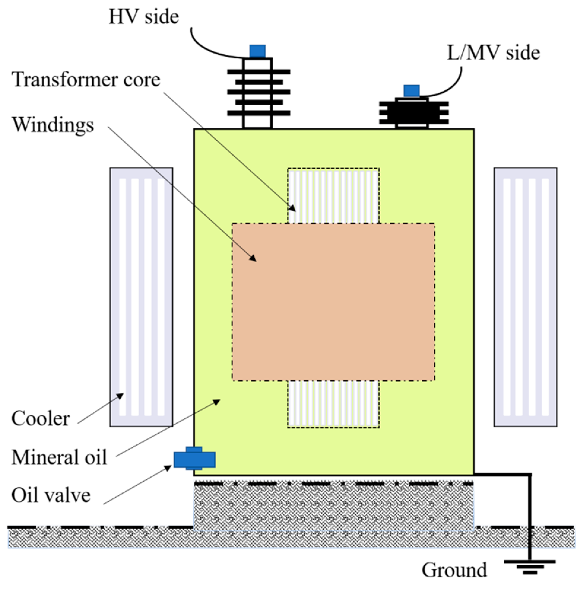
2. Problem Formulation

Highly reliable transformers are mainly made of iron core and windings; both are placed in the oil tank filled with insulating oil, as shown in Figure 1.

Mineral insulating oil is the most common type of oil used in outdoor transformers [19]. This insulating oil has significant dielectric strength so that it can withstand a pretty high voltage. It also reduces heat generated by transformer windings employing the cooler (radiators, air fans, …). Therefore, the heat generated in the transformer results in a temperature rise in the internal transformer structures. Under electrical and thermal stresses, different hydrocarbon gases are liberated due to the insulating oil decomposition. Particular gases characterize each type of fault. For instance, hydrogen concentration, produced by ionic bombardment, increases with partial discharges within a transformer oil. In this context, a general review about the gases produced during the deterioration of mineral oil and their interpretation has been detailed in [10].

Early-stage detection of these faults should be carried out to avoid the undesired abnormal operating conditions or transformer outages. For this purpose, periodic monitoring of the oil should be conducted during transformer service, whether in-situ or at the laboratory, using a multi-stage gas-extractor (a device for sampling transformer oil) [10]. In general, the most important gases are Hydrogen (H₂), Methane (CH₄), Acetylene (C₂H₂), Ethylene (C₂H₄), and Ethane (C₂H₆). The distribution of these gases is related to the type of transformer fault, and the rate of gas generation can indicate the severity of the fault [5,20].

In [6], the authors have collected 481 samples associating with the six different faults as indicated in the Introduction (i.e., PD, D1, D2, T1, T2, and T3). The number of samples associated with each fault is given in

Table 1. Database distribution.

Defect	Interpretation	Number of Samples
PD	Partial discharge	48
D1	Low energy discharges	79
D2	High energy discharges	126
T1	Thermal faults of <300 °C	95
T2	Thermal faults of 300 °C to 700 °C	48
T3	Thermal faults of >700 °C	85
All		481

.

The database set has been exploited in the present investigation to detect and identify faults. As shown in this table, only separated faults (no combined faults) have been considered. The fault detection has been examined using the concentration of each dissolved gas. Since the weight percent of the gases as mentioned earlier would result in an inopportunely small number, concentration in parts per million, or ppm, has been considered for each gas. Furthermore, percent concentration of the total sum was also used, where each sample X = [x₁, x₂, …, x₅] is scaled as follows:

$$X =\frac{X}{{{\displaystyle \sum }}_{i=1}^5{x}_i}\times 100\%$$

(1)

The faults diagnostic method has been carried out elaborating two different classifiers, namely Gaussian and SVM-BA. The flowchart given in Figure 2 summarizes the various stages of the diagnostic approach.

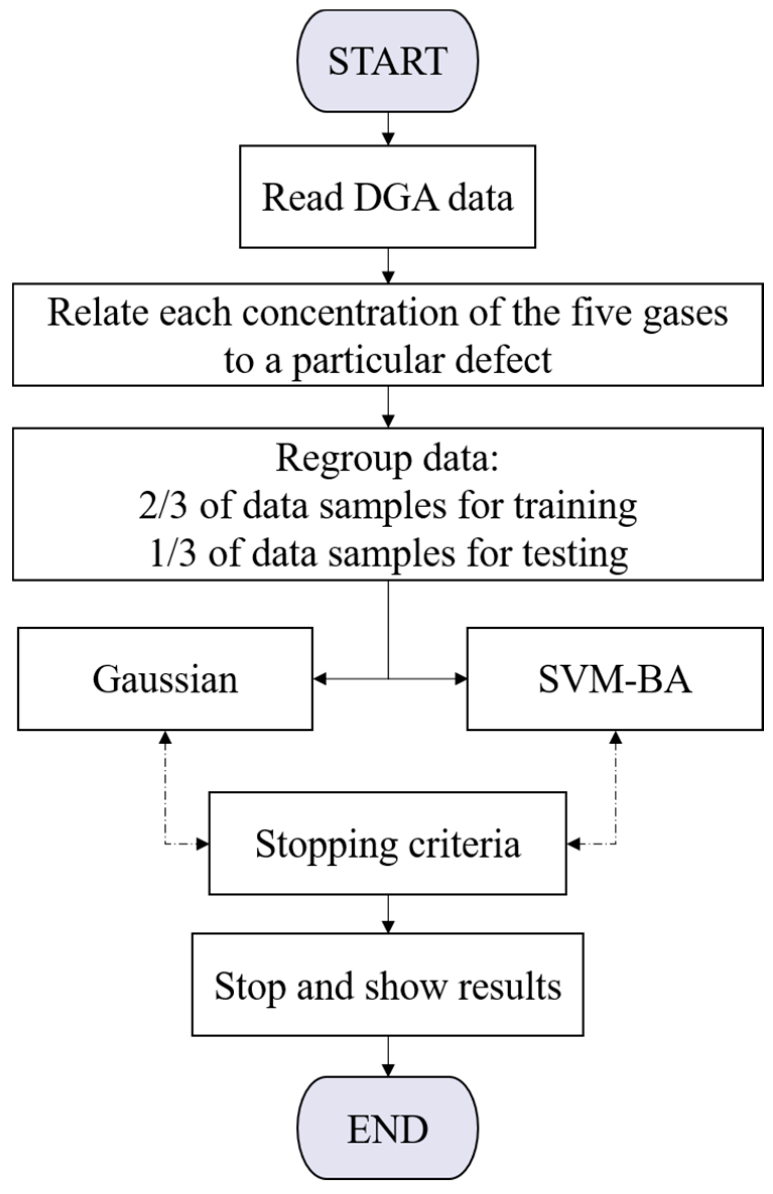
3. Classification Approach

For both, Gaussian and SVM-BA, classifier, the concentrations in percentages and ppm of the five dissolved gases have been used as an input vector, denoted by X = [x₁, x₂, …, x₅], associated with a particular class of fault (denoted by y) representing the classifier decision (classifier output).

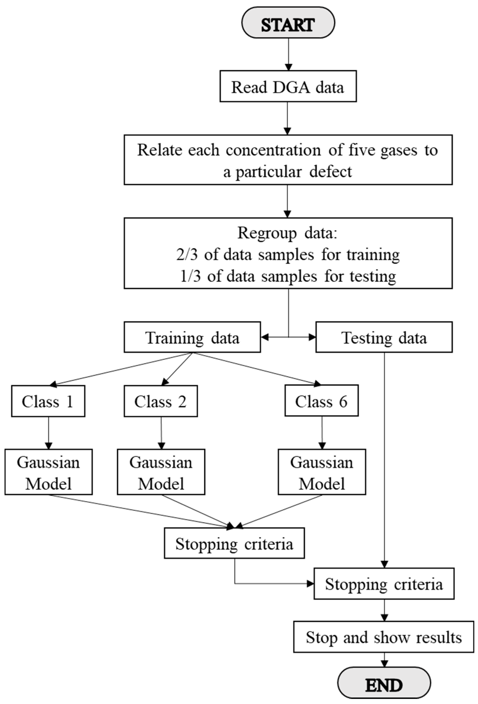
3.1. Gaussian Classifier

In this part, the Gaussian classification is used as a probabilistic learning method for constructing a classifier by applying Bayes’ theorem. It concerns the conditional and marginal probabilities of two random events. The classifier is based on the comparison of the posterior probability P (w_i|x):

$$P\left(w_i|x\right)=\frac{P\left(x|w_i \right)P\left(w_i\right)}{P\left(x\right)}, i=1,2, \dots ,6$$

(2)

where P (x|w_i) is the conditional probability (likelihood) given by:

$$P(x|w_i)={\displaystyle \prod }_{k=1}^{6}P(x_k|w_i)$$

(3)

and P(x) is the unconditional density that normalizes the posteriors, computed as follows:

$$P\left(x\right)={\displaystyle \sum }_{i=1}^{6}P(x|w_i)P\left(w_i\right)$$

(4)

in which P(w_i) is the prior probability of each class.

Firstly, the training phase has been carried out for constructing the parameters of the Gaussian model. In this phase, 321 samples of the data set have been reserved to determine the Gaussian distributions, consisting of the mean value (µ) and the matrix covariance (σ) of the gas concentration for each defect class. Since the number of samples differs from one fault to another, every distribution is multiplied by a weight corresponding to its samples’ number on the database’s total size.

In the next step, Gaussian has been employed to compute the conditional probability P (x|w_i) as indicated in Equation (3), where the posterior probability is calculated using the probability density function of a univariate normal distribution as follows:

$$P(x_{ij}|w_k)=\frac{1}{\sqrt{2\pi {\sigma }^2}}{e}^{-\frac{1}{2}\frac{{(x_k-m)}^2}{{\sigma }^2}}$$

(5)

Since it is required to know the likelihood of observing the k-th sample while considering all the different distributions, one can sum the likelihood of observing the given sample from each possible Gaussian, using:

$$P(x_k|w_i)=\frac{exp[-\frac{1}{2}\left(X-\mu {)}^T{\sigma }^{-1}\left(X-\mu \right)\right]}{{(2\pi )}^{6/2}\sqrt{\left|\sigma \right|}}$$

(6)

in which, |σ| and σ⁻¹ denote the determinant and inverse of the covariance matrix σ.

Each Gaussian model’s parameters (i.e., variance, mean, and weight) have been addressed to cluster the data and estimate those having the same parameters. Moreover, a maximum likelihood estimate (MLE) was used to find the optimal mean and variance, maximizing the data’s likelihood. After training the model, the classifier output ideally ends up with six distributions on the same axis. Depending on the axis’s location, each testing sample (a total of 160 testing ones) is placed in one of the defect classes. Figure 3 illustrates the different steps of the Gaussian classifier.

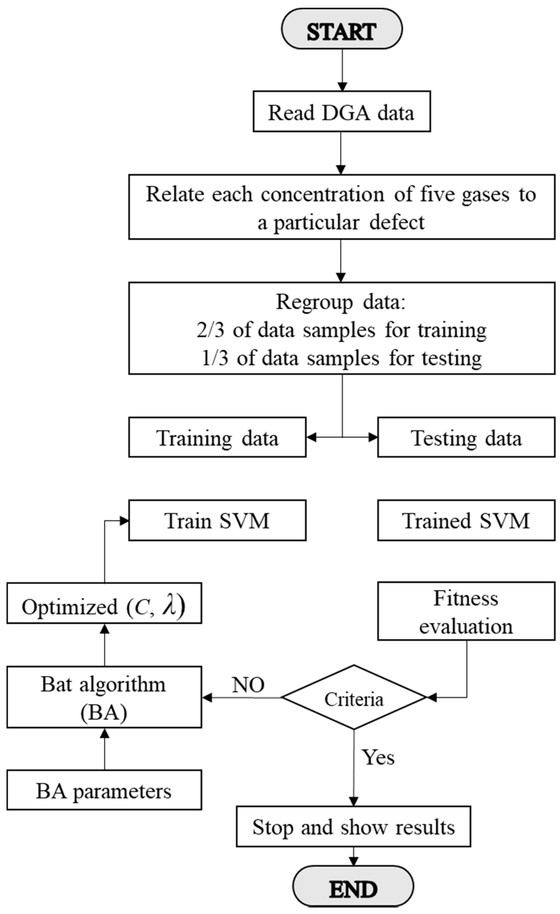
3.2. SVM Classifier Coupled with BA

SVMs techniques are used in the problem of classification, regression, and prediction models [21]. For the classification problems, hyperplanes are required in a multidimensional space separating data points of both fault classes. These hyperplanes are used to distinguish between every two classes (y_i and y_j) of faults associated with two different input vectors (X_i and X_j) [22,23,24]. Among these hyperplanes, it is suggested to find the one that has the maximum margin (denoted by M). In this light, the classification becomes an optimization problem where hyperplanes represent the decision boundaries that help classify the data points. Usually, an orthogonal vector (denoted by ω) to the hyperplane defined by:

$$\omega =\left[{\omega }_1,{\omega }_2,\dots ,{\omega }_k\right]$$

(7)

which is used in combination with an input vector (Xi) to define the hyperplane function, h, as follows [22]:

$$h\left(X_i\right)=w^T. X_i+{\omega }_0={\omega }_0+{\displaystyle \sum }_{i=1}^k{\omega }_i.x_i$$

(8)

The ${\omega }_0$ is the bias term required to determine the position of separating hyperplane (i.e., h (X) = 0).

A learning strategy of One-to-One is selected. It is assumed that X_i is of class “1” if h (X_i) ≥ 0 and, consequently, it is of class “−1” elsewhere. Assuming that X_i and X_j are the two closest points on each side of the hyperplane (different classes), the equations for the hyperplanes h (X_i) and h (X_j) become:

$$h\left(X_i\right)=w^T. X_i+{\omega }_0=1$$

(9)

and

$$h\left(X_i\right)=w^T. X_i+{\omega }_0=-1$$

(10)

Differencing these equations and dividing both sides by the magnitude of the ω, we obtain:

$$X_i{-\mathrm{X}}_j=\frac{2}{\left|\left|\omega \right|\right|}$$

(11)

X_i − X_j is the distance between the two hyperplanes.

From the expression (11), it is clear that the maximization of the margin implies the minimization of the weight vector ω used to define the hyperplane. A soft-margin SVM is utilized for nonlinear classes to provide freedom to the model misclassifying some data points by minimizing the number of such samples [23]. For this purpose, slack variable non-negatives ζ_i is introduced in the hyperplane equation. Consequently, the optimization problem becomes:

$$\{\begin{array}{l}Min:\frac{1}{2}{\Vert \omega \Vert }^2+C{\displaystyle {\displaystyle \sum }_{i=1}^k}{\zeta }_i\\ Such that : y_i\left(\omega .x_i+{\omega }_0\right)\ge 1-{\zeta }_i\\ \forall i, 0 < {\zeta }_i < 1 i=1,2,\dots ,k\end{array}$$

(12)

C represents the margin parameter, which can be seen as a regularization parameter. The corresponding Lagrangian dual problem is given by:

$$L\left(\omega ,{\omega }_0,\zeta ,\alpha \right)=\frac{1}{2}{\Vert \omega \Vert }^2+C {{\displaystyle \sum }}_{i=1}^k{\zeta }_i-{{\displaystyle \sum }}_{i=1}^k{\alpha }_i[y_i\left({\omega }_i{x}_i+{\omega }_0\right) - 1+{\zeta }_i)$$

(13)

α_i are Lagrange coefficients (multipliers).

In such circumstances, the Karush–Kuhn–Kucker conditions are [14]:

$$L\left(\omega ,{\omega }_0,\zeta ,\alpha \right)=\frac{1}{2}{\Vert \omega \Vert }^2+C {{\displaystyle \sum }}_{i=1}^k{\zeta }_i-{{\displaystyle \sum }}_{i=1}^k{\alpha }_i[y_i\left({\omega }_i{x}_i+{\omega }_0\right) - 1+{\zeta }_i)$$

(14)

Setting the derivatives as mentioned earlier of the Lagrangian and ${\omega }_0$ individually to 0, it follows that the Lagrangian expression should be maximized under the constraint:

$${\displaystyle \sum }_{i=1}^k{\alpha }_i{y}_i=0$$

(15)

and it also yields

$$C={\alpha }_i+{\zeta }_i$$

(16)

Since the data are assumed as non-separable, the feature space has been enlarged by a characteristic function Φ known as Kernel function. Every data point has been mapped into high-dimensional space through a particular transformation Φ: X 7→ ϕ (X). Polynomial Kernel function of d–degree has been used in this investigation as follows [23]:

$$K\left(x_i,x_j\right)={(C+x.x^{\prime })}^d$$

(17)

which verifies the following condition:

$$\varphi \left(x_i\right).\varphi \left(x_j\right)=K\left(x_i,x_j\right)$$

(18)

In this case, the optimization problem after rearrangement becomes as follows:

$$\{\begin{array}{l}Max:{\displaystyle {\displaystyle \sum }_{i=1}^k}{\alpha }_i-\frac{1}{2}{\displaystyle {\displaystyle \sum }_{i=1}^k}{\displaystyle {\displaystyle \sum }_{j=1}^k}{\alpha }_i{\alpha }_j{y}_i{y}_j\Phi \left(x_i\right)\Phi \left(x_j\right) \\ Subject to : \forall i\in \left\{1,2, \dots ,k\right\}, C\ge {\alpha }_k\ge 0\\ {\displaystyle {\displaystyle \sum }_{i=1}^m}{\alpha }_i.x_i=0\end{array}$$

(19)

SVM parameters consisting in:

• Kernel parameter λ (conditioning parameter equivalent σ in RBF kernel [24]);
• penalty parameter C (margin parameter); and
• degree d of the Kernel polynomial.

significantly affect the accuracy of predicting model. To further improve the accuracy rate, the bat algorithm (BA) has been elaborated in this investigation to optimize the SVM parameters. BA is part of meta-heuristic algorithms for global optimization, intended (by Xin-She Yang in 2010) to simulate prey’s sensing distance and avoid obstacles using microbats echolocation behavior [23]. In BA, the aim is reached by determining the optimum parameters C and λ that give the best accuracy rate of the SVM classifier. The degree of a polynomial kernel has been fixed at d = 1, 2, and 3. Figure 4 illustrates the different steps of the coupled SVM-BA classifier.

In the beginning, BA parameters have been initialized.

Table 2. Parameters of Bat algorithm.

Parameter	Value
Population size	50
Loudness	0.5
Frequency (fmin and fmax)	0 and 20
Number of iterations	600
Pulse rate	0.5

lists the detailed settings for the BA values used to optimize the SVM model.

Therefore, BA generates a population of the SVM parameters (C, λ). For each couple, the initial position p and velocity v have been randomly selected. Each couple’s fitness has been evaluated to extract the best global position (denoted by p∗). This means that the training dataset is used to train the SVM classifier for each position, while the testing dataset is used to calculate the accuracy rate. This latter represents the ratio between the number of correctly classified samples (N_c) to the total number of test samples (N). After this step, the position and velocity of each individual are updated using the following expressions:

$$\{\begin{array}{l}{p}_i^{t+1}=p_i^t+v_i^t \\ v_i^{t+1}=v_i^t+(p_i^t-p^{*})f_i\end{array}$$

(20)

where v_i^t and v_i^t+1 are current, and the next velocities correspond to the existing p_i^t and the next p_i^t+1 positions, respectively.

The parameter f_i denotes the frequency, which is computed as follows:

$$f_i=f_{min}+(f_{max}-f_{min})\beta$$

(21)

in which β is a random number ranging between 0 and 1.

It is worth noting that the searching space has been bounded by C_min = 10⁻⁶ and C_max = 0.1 for the parameter C against λ_min = 10⁻⁷ and λ_max = 0.7 for the second parameter λ. Moreover, the pulse rate increased according to the iteration number as follows:

$$r_i^{t+1}=r_i^0+\left[1-\exp (-\gamma t\right)]$$

(22)

while the loudness decreased by:

$$A_i^{t+1} = \sigma A_i^0,\hspace{1em} 0\sigma <1$$

(23)

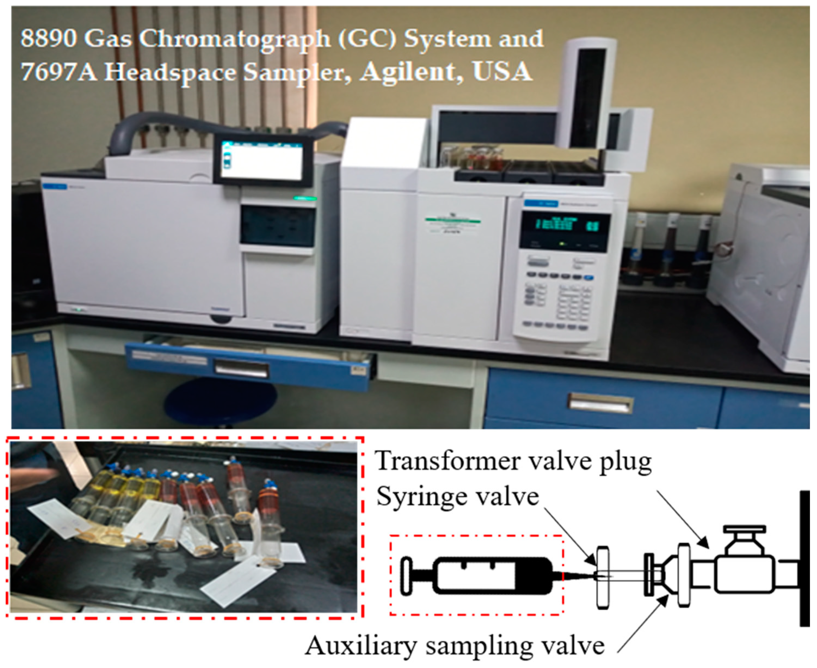
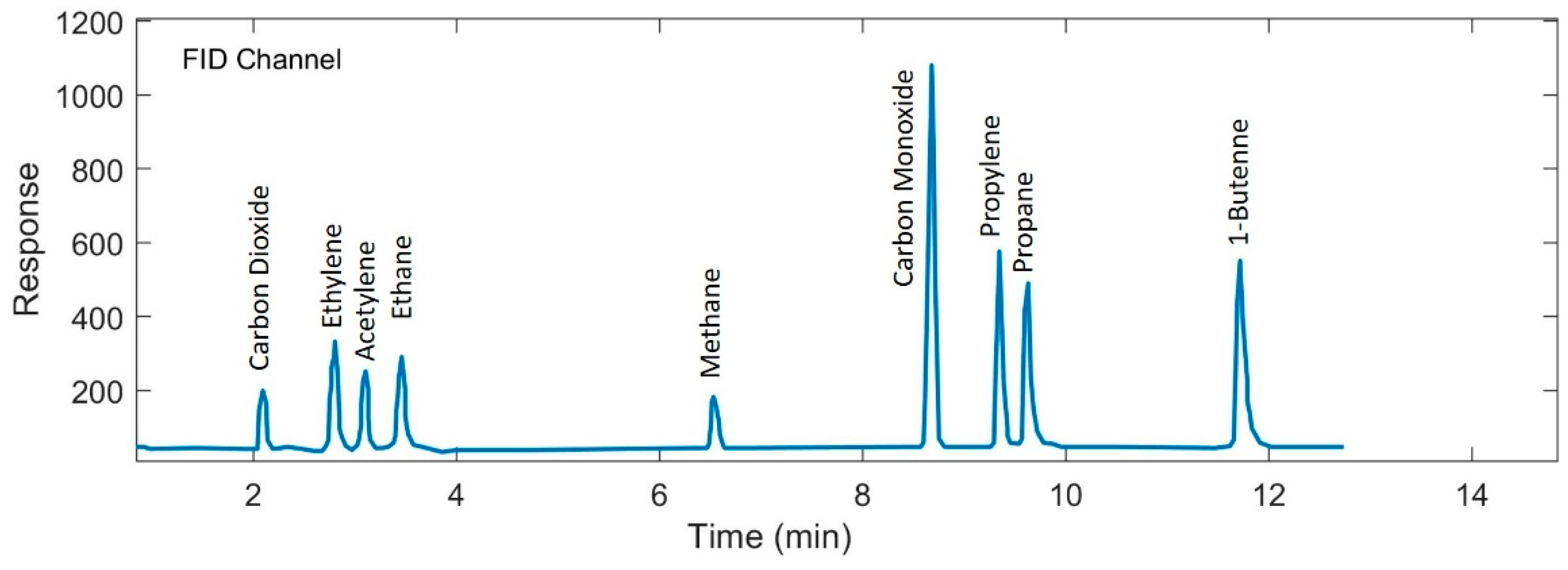
4. Experimental Work

During transformers’ operation, the insulation of transformer coils is subjected to high electrical and thermal stresses causing corrosion of some insulating material particles and decomposition of some insulating oil particles producing different types of gases. These gases dissolve in the transformer oil. At the beginning of any slight fault, the gases are not released largely enough to operate the gas protection device that does not cause instantaneous breakdown, but the transformer efficiency is reduced.

The gases that were used to diagnose the transformers’ state include Hydrogen (H₂), Methane (CH₄), Acetylene (C₂H₂), Ethylene (C₂H₄), Ethane (C₂H₆), carbon monoxide (CO), and carbon dioxide (CO₂). Hence, chromatographic analysis (CA) of dissolved gases in transformer oils is considered as an analysis method that reveals small percentages of dissolved gases in the oil. The CA of gases indicates the transformers’ condition in the early stage of the fault occurrence. Thus, the transformers can be preserved and decrease the transformer failure before a transformers’ complete breakdown occurs.

The CA results’ accuracy depends on drawing the transformer’s oil sample, extracting the dissolved gases from the oils’ samples, and adjusting the analyzer device. The CA must be carried out at the start of the transformers’ operation, and its results are considered a reference when analyzing this transformer later.

American Society for Testing and Materials (ASTM) D3612-2 [24] indicates the dissolved gases’ extracting procedures from the transformer oils’ samples using gas chromatography (GC). The GC consists of the mobile phase (including three types of gases the carrier gas, the fuel gas, and zero air), the sample injector, the column, the columns’ oven, the detector, and the data system.

Oil samples were prepared and filled with glass vials by a sampling device. Then, they were placed into the Autosampler unit. Hence, one by one, the samples were analyzed, and inserted into the oven at 80 °C. The dissolved gases are extracted by increasing the temperature by moving the oil sample. Hence, the extracted gases are injected into the GC to accomplish the gases’ analysis [25].

Figure 5 illustrates the oil samples’ drawing process from the transformer and the GC device (8890 Gas Chromatograph (GC) System and 7697A Headspace Sampler, Agilent, USA). The GCs’ analysis results are shown in Figure 6, illustrating the time required to extract each gas and its concentration in ppm. The chromatograph provides a signal with time, which produces the familiar chromatogram. The chromatogram signal can be converted into a list of peak times and sizes by either manual or electronic means [26].

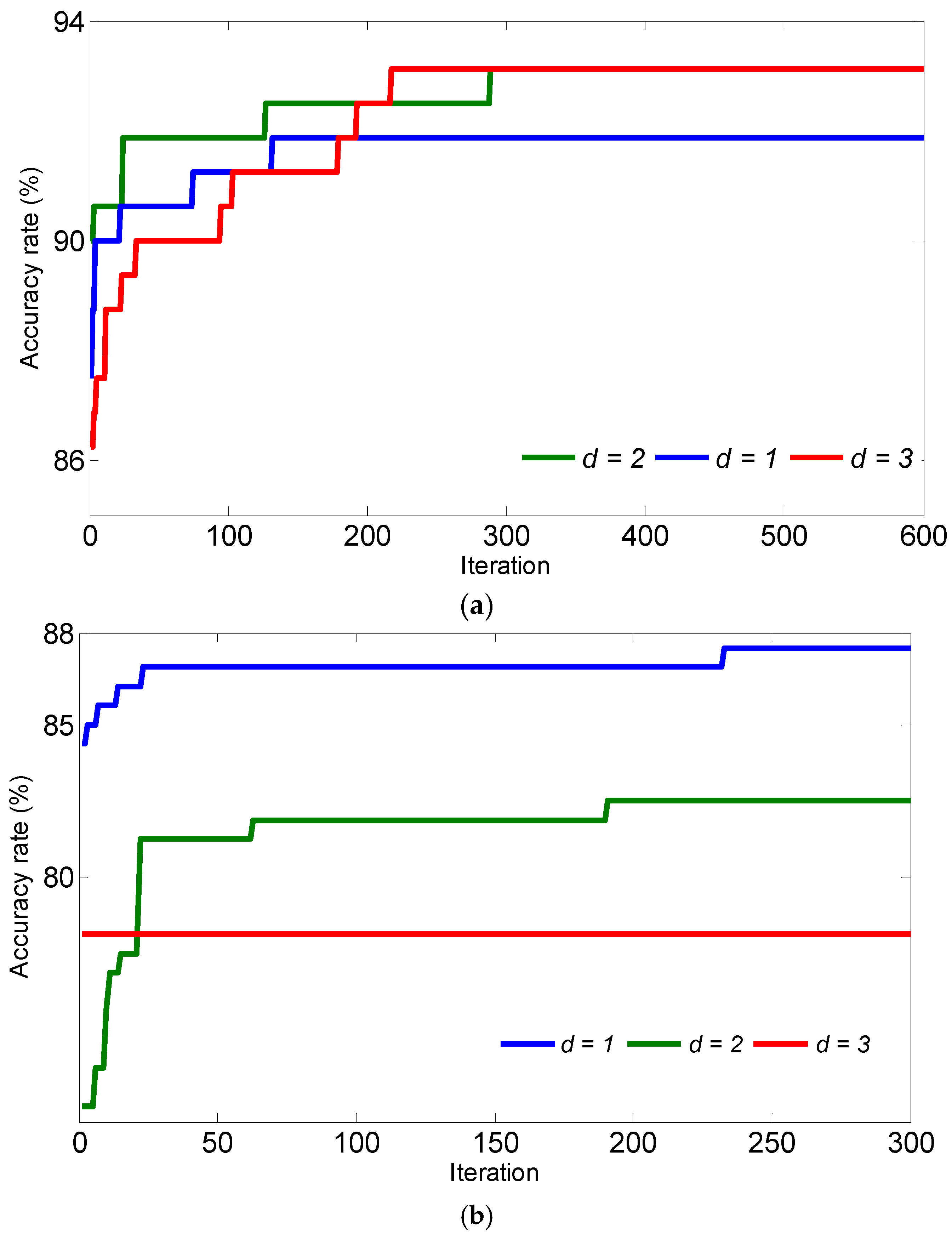
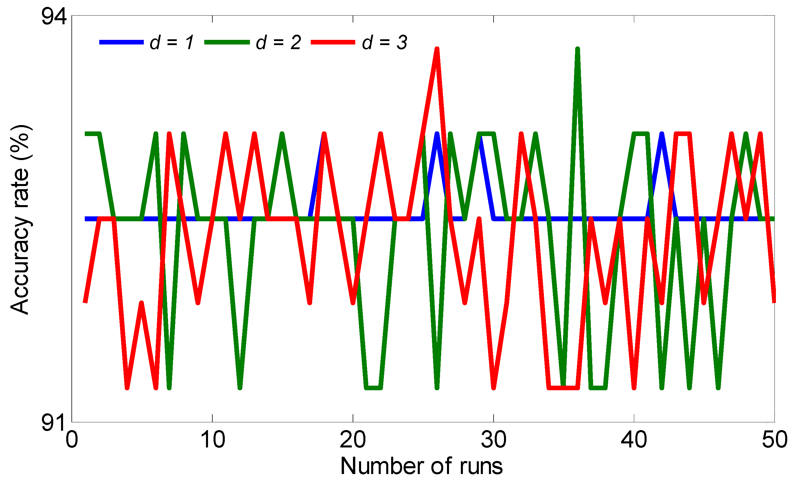
5. Results and Discussions

A database set of 481 samples has been exploited to evaluate each classifiers’ accuracy rate. As stated in Section 2, 321 samples of the data set were used in the training phase, while the rest was used for testing (160 samples). The data distribution was based on the holdout method; more than 60% of the database must be reserved for the training phase (2/3 for the training set and the remaining 1/3 as the test set) [27]. Both data parts were randomly selected, and they were used in all simulations. DGA results in percentages (i.e., percentages of the total sum) and ppm have been considered an input vector for both classifiers. As mentioned previously for SVM, the Kernel polynomial and a one-to-one learning strategy were selected. The classifiers’ results were compared regarding inspection (the real fault in the transformer) as in

Table 3. Diagnosis results of some cases.

H2	CH4	C2H2	C2H4	C2H6	Inspection	SVM-BA (Input Vector in ppm)	Gaussian (Input Vector in ppm)	SVM-BA (Input Vector in Percentage)	Gaussian (Input Vector in Percentage)
2587.2	112.25	0	1.4	4.704	PD	PD	D2 *	PD	PD
6870	1028	5500	900	79	D1	D1	D1	D1	D2 *
84	6	86	14	1	D2	D2	T3 *	D1 *	D1 *
92	27	0	7	67	T1	T1	T3 *	T1	T1
960	4000	6	1560	1290	T2	T3*	T3 *	T2	T3 *
1374	2648	298	5376	628	T3	T3	T3	T3	T3

(*) denotes that diagnosis is wrong based on the inspection.

. In Table 3, some cases were illustrated to explain the comparison between the SVM-BA and Gaussian classifier for gases in ppm and gases percentages.

Not only the type of input vector influences the accuracy rate in the SVM algorithm, but in the experience of previous investigations, the degree of the polynomial kernel can also affect the diagnostic accuracy [28]. Figure 7 shows the impact of vector input type on the classification performance for the SVM-BA classifier’s evolution during the optimization process. This latter has been illustrated in Figure 7a,b when the input vector calculates gases in percentages and ppm, respectively, with different polynomial kernel degrees.

For a given degree of Kernel polynomial, it is clear that 300 iterations are mainly sufficient for the convergence of the SVM-BA algorithm. The results showed that the SVM-BA classifier’s accuracy rate is quite sensitive to the degree of Kernel polynomial. For an input vector taken in percentages as shown in Figure 7a, the maximal accuracy rate is 93.13% with d = 2 and 3 against 91.88% with d = 1. On the other hand, notably lower results have been found in Figure 7b for an input vector in ppm where the highest accuracy is 87.5% obtained for d = 1 against 82.5% and 78.13% for d = 2 and 3, respectively. However, the convergence for d = 3 is very fast compared to those found for d = 2 and d = 1.

The previous simulation, related to the SVM-BA classifier and shown in Figure 7, is repeated 50 times to find the best accuracy rate to provide more credibility of the obtained results. Figure 8 illustrates an example of the accuracy rate versus the number of runs (i.e., executions) when using DG in percentages as an input vector for the SVM-BA classifier. These results have been computed for the Kernel polynomial of d = 1, 2, and 3 degrees.

In Figure 8, the best accuracy rate obtained for different executions is located between 91% and 94%. The global best results related to the accuracy rate obtained for several runs are presented in

Table 4. The accuracy rate for both classifiers after 50 executions.

Classifier	Gaussian	SVM-BA
		d = 1	d = 2	d = 3
DGA in percentages	69.37 %	93.13%	93.75%	93.75%
DGA in ppm	32.75 %	87.50%	82.50%	78.13%

. Additionally, DGA has been elaborated in ppm and percentages for the input vector.

For SVM-BA, the results are given for three degrees of Kernel polynomial. After 50 executions, it was found that the maximal accuracy rate was 93.75% with d = 2 and 3 against 93.13% with d = 1 obtained when employing an input vector in percentages. When using the dissolved gases in ppm as input vector for the SVMBA, the computed results decreased to 87.50% for d = 1 against 89.75% for d = 2 and 3. This implies that the SVM-BA classifier gives a better accuracy rate for an input vector given in percentages. On the other hand, Gaussian classifier gives the lowest accuracy rate of 32.75% when the input vector employed in ppm compared to an accuracy rate of 66.25% when the input vector is in percentages. This ascertainment demonstrates the concentration of gases in percentages to differentiate between a particular defect from the other ones.

For the Gaussian classifier, it should be noted that the results have been dramatically improved when the real part of the posterior probability given by the expression (6) is employed. In this case, the accuracy rate has been increased to 70% for percentages input in while it remains the same (i.e., 32.75%) for an input vector in ppm. Such findings suggest using the real part of posterior Probability in Gaussian classifier with an input vector in percentages. Compared to other literature results, the SVM-BA classifier has good accuracy and has high abilities to diagnose the transformer fault classes with simple codes. The overall accuracy obtained in [6] for the same database in ppm is a good example of this.

6. Validation and Overall Accuracy of the Proposed SVM-BA Classifier

The SVM-BA and Gaussian classifiers are compared with various classification algorithms used in the DGALab interface to evaluate the proposed method’s accuracy [17]. The free DGALab software package is available in [18]. DGALab involves the Duval triangle method, IEC code 60599, Roger’s four ratios, modified IEC code and Modified Rogers’ 4 ratios, clustering method, conditional probability, and California State University Sacramento artificial neural network method (CSUS-ANN). The details of the whole algorithms are cited in [15,16,17]. A comparison among all these mentioned methods was carried out based on the individual fault accuracy and overall accuracy rate (

Table 5. Accuracy rate table of different techniques.

	ACT	Duval Triangle	IEC Code-60599	Rogers’ 4 Ratios	Modified IEC Code	Modified Rogers’ 4 Ratios	Clustering	Conditional Probability	CSUS ANN	SVM-BA	Gaussian
PD	16	93.75	43.75	37.5	8.5	75	93.75	100	8.5	87.5	81.25
D1	26	76.92	26.92	0	76.92	84.61	84.61	76.92	69.23	92.31	34.61
D2	42	85.71	66.66	73.80	90.47	88.09	85.71	97.61	92.85	95.24	78.57
T1	32	65.62	53.125	90.62	93.75	93.75	93.75	87.5	93.75	93.75	90.62
T2	16	50	68.75	25	93.75	93.75	31.25	81.25	43.75	87.5	0
T3	28	100	82.14	57.14	89.28	89.28	85.7	82.14	71.42	96.48	100
All	160	80	58.12	53.75	88.75	88.12	82.5	88.12	80	93.75	69.37

).

The last row in Table 5 illustrates the total number of samples used for testing purposes and the overall accuracy of each DGA method for comparison purposes. From the evaluation exposed in Table 5, the SVM-BA provides the best overall accuracy rate (93.75%). This superiority came from the ability of SVM to classify the complex and extensive data set. Moreover, the coupling of SVM with the BAT algorithm enabled the right choice of parameters which gave the highest possible accuracy rate. The nearest overall accuracy of the proposed method is the modified IEC code, which showed an 88.75% overall accuracy rate. The worst overall accuracy rate is the Rogers’ four ratio DGA method, for which the overall accuracy is 53.75%. The results in Table 5 are recapitulated in Figure 9 in a histogram form.

7. Conclusions

This paper proposed a new DGA technique using an SVM-BA classifier to enhance the transformer faults’ diagnostic accuracy. Five main combustible dissolved gas concentrations (H₂, CH₄, C₂H₆, C₂H₄, and C₂H₂) were used as an input vector top the SVM-BA classifier to identify the transformer fault type. The concentration of five dissolved gases was used in ppm and in percentages. A total of 481 samples was collected from the chemical laboratory and literature, categorized into 321 data samples for training and 160 data samples for testing processes. The SVM-BA classifier results indicated the following:

• An accuracy rate of 93.75% has been achieved when the input vector in percentage with d = 2 and 3 degrees.
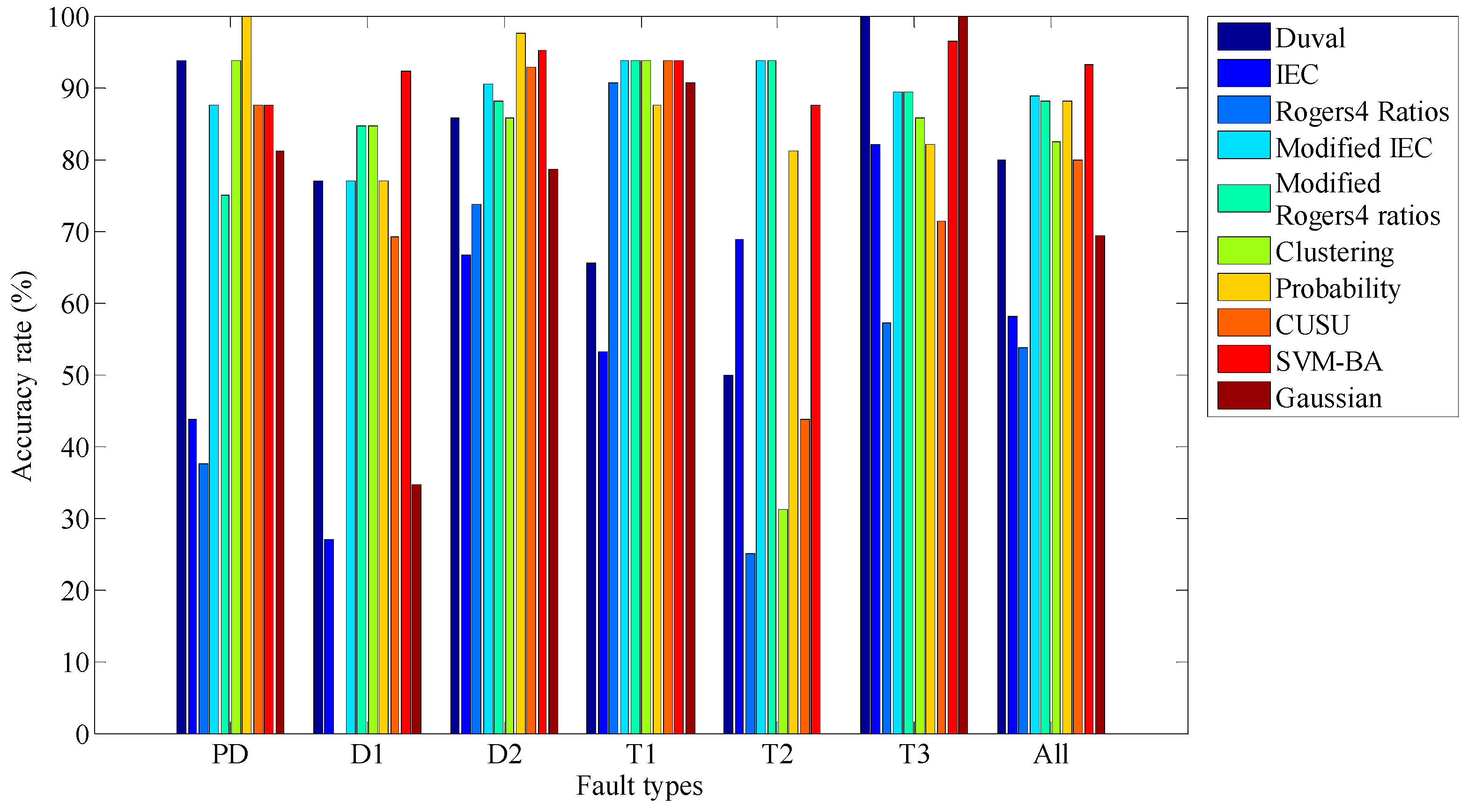
• The coupled SVM-BA classifier’s test results revealed the classifier’s ability to enhance the transformer faults’ diagnostic accuracy rather than the other DGA techniques in the literature.
• The overall accuracy of SVM-BA was 93.75%, which is higher than that of the modified IEC code (88.75%).
• It recommended determining the expected remaining life of the transformer based on the state of the insulation system.

References

1. Benmahamed, Y.; Teguar, M.; Boubakeur, A. Application of SVM and KNN to Duval Pentagon 1 Transformer Oil Diagnosis. IEEE Trans. Dielect. Electr. Inst. 2017, 24, 3443–3451. [Google Scholar] [CrossRef]
2. Ji, X.; Zhang, Y.; Liu, Q. Insulation Condition Assessment of Power Transformers Employing Fused Information in Time and Space Dimensions. Electr. Power Comp. Syst. 2020, 48, 213–223. [Google Scholar] [CrossRef]
3. Malik, H.; Mishra, S. Selection of Most Relevant Input Parameters Using Principal Component Analysis for Extreme Learning Machine Based Power Transformer Fault Diagnosis Model. Electr. Power Compon. Syst. 2017, 45, 1339–1352. [Google Scholar] [CrossRef]
4. IEEE Standard C57-104. Guide for the Interpretation of Gases Generated in Oil-Immersed Transformers; IEEE: New York, NY, USA, 2008; p. 104. [Google Scholar]
5. Jiang, J.; Chen, R.; Zhang, C.; Chen, M.; Li, X.; Ma, G. Dynamic Fault Prediction of Power Transformers Based on Lasso Regression and Change Point Detection by Dissolved Gas Analysis. IEEE Trans. Dielect. Electr. Inst. 2020, 27, 2130–2137. [Google Scholar] [CrossRef]
6. Taha, I.B.M.; Hoballah, A.; Ghoneim, S.S.M. Optimal ratio limits of Rogers’ four-ratios and IEC 60599 code methods using particle swarm optimization fuzzy-logic approach. IEEE Trans. Dielect. Electr. Inst. 2020, 27, 222–230. [Google Scholar] [CrossRef]
7. Gouda, O.E.; El-Hoshy, S.H.; ELTamaly, H.H. Condition assessment of power transformers based on dissolved gas analysis. IET Gener. Trans. Distrib. 2019, 13, 2299–2310. [Google Scholar] [CrossRef]
8. Code, P.; Prix, C. Mineral Oil-Impregnated Electrical Equipment in Service–Guide to the Interpretation of Dissolved and Free Gases Analysis; IEC Publication 60599; British Standards Institution: London, UK, 2007. [Google Scholar]
9. Duval, M.; Lamarre, L. The Duval Pentagon—A new Complementary Tool for the Interpretation of Dissolved Gas Analysis in Transformers. IEEE Electr. Insul. Mag. 2014, 30, 9–12. [Google Scholar]
10. Cheim, L.; Duval, M.; and Haider, S. Combined Duval Pentagons: A Simplified Approach. Energies 2020, 13, 2859. [Google Scholar] [CrossRef]
11. Mansour, D.A. Development of a new graphical technique for dissolved gas analysis in power transformers based on the five combustible gases. IEEE Trans. Dielect. Electr. Inst. 2015, 22, 2507–2512. [Google Scholar] [CrossRef]
12. Benmahamed, Y.; Kemari, Y.; Teguar, M.; Boubakeur, A. Diagnosis of Power Transformer Oil Using KNN and Nave Bayes Classifiers. In Proceedings of the 2018 IEEE 2nd International Conference on Dielectrics (ICD), Budapest, Hungary, 1–5 July 2018. [Google Scholar]
13. Poonnoy, N.; Suwanasri, C.; Suwanasri, T. ‘Fuzzy Logic Approach to Dissolved Gas Analysis for Power Transformer Failure Index and Fault Identification. Energies 2021, 14, 36. [Google Scholar] [CrossRef]
14. Benmahamed, Y.; Teguar, M.; Boubakeur, A. Diagnosis of Power Transformer Oil Using PSO-SVM and KNN Classifiers. In Proceedings of the 2018 International Conference on Electrical Sciences and Technologies in Maghreb (CISTEM), Algiers, Algeria, 28–31 October 2018. [Google Scholar]
15. Ghoneim, S.S.M.; Taha, I.B.M. A new approach of DGA interpretation technique for transformer fault diagnosis. Int. J. Electr. Power Energy Syst. 2016, 81, 265–274. [Google Scholar] [CrossRef]
16. Taha, I.B.M.; Mansour, D.A.; Ghoneim, S.S.M.; Elkalashy, N. Conditional probability-based interpretation of dissolved gas analysis for transformer incipient faults. IET Gener. Transm. Distrib. 2017, 11, 943–951. [Google Scholar] [CrossRef]
17. Ibrahim, S.; Ghoneim, S.S.M.; Taha, I.B.M. DGALab: An extensible software implementation for DGA. IET Gener. Transm. Distrib. 2018, 18, 4117–4124. [Google Scholar] [CrossRef]
18. Ibrahim, S.; Taha, I.B.M.; Ghoneim, S.S.M. DGA Tool GitHub Repository. 2018. Available online: https://github.com/Saleh860/DGA (accessed on 19 May 2021).
19. IEEE Std C57-104. IEEE Guide for the Reclamation of Mineral Insulating Oil and Criteria for Its Use; British Standards Institution: London, UK, 2015; p. 637. [Google Scholar]
20. Wani, S.A.; Khan, S.A.; Prashal, G.; Gupta, D. Smart Diagnosis of Incipient Faults Using Dissolved Gas Analysis-Based Fault Interpretation Matrix (FIM). Arab. J. Sci. Eng. 2019, 44, 6977–6985. [Google Scholar] [CrossRef]
21. Yazdani-Asrami, M.; Taghipour-Gorjikolaie, M.; Song, M.; Zhang, W.; Yuan, W. Prediction of Nonsinusoidal AC Loss of Superconducting Tapes Using Artificial Intelligence-Based Models. IEEE Access 2020, 8, 207287–207297. [Google Scholar] [CrossRef]
22. Wei, H.; Wang, Y.; Yang, L.; Yan, C.; Zhang, Y.; and Liao, R. A new support vector machine model based on improved imperialist competitive algorithm for fault diagnosis of oil-immersed transformers. J. Elect. Eng. Technol. 2017, 12, 830–839. [Google Scholar]
23. Tharwat, A.; Hassanien, A.E.; Elnaghi, B. A BA-based algorithm for parameter optimization of Support Vector Machine. Pattern Recognit. Lett. 2017, 93, 13–22. [Google Scholar] [CrossRef]
24. Liu, T.; Zhu, X.; Pedrycz, W.; Li, Z. A design of information granule-based under-sampling method in imbalanced data classification. Soft Comput. 2020, 24, 17333–17347. [Google Scholar] [CrossRef]
25. ASTM. Standard Test Method for Analysis of Gases Dissolved in Electrical Insulating Oil by Gas Chromatography; D3612-2; ASTM: West Conshohocken, PA, USA, 2017. [Google Scholar]
26. Available online: https://www.agilent.com/cs/library/usermanuals/public/G1176-90000_034327.pdf (accessed on 19 May 2021).
27. Foysal, K.H.; Chang, H.J.; Bruess, F.; Chong, J.W. SmartFit. Smartphone Application for Garment Fit Detection. Electronics 2021, 10, 97. [Google Scholar] [CrossRef]
28. Ali, S.; Smith, K.A. Automatic parameter selection for polynomial kernel. In Proceedings of the Fifth IEEE Workshop on Mobile Computing Systems and Applications, Las Vegas, NV, USA, 27–29 October 2003; pp. 243–249. [Google Scholar]
Figure 1. Oil-immersed power transformer cross-section.
Energies 14 02970 g001
Figure 2. Flowchart of the problem formulation.
Energies 14 02970 g002
Figure 3. Flowchart formulating the problem using Gaussian classifier.
Energies 14 02970 g003
Figure 4. Flowchart formulating SVM-BA Classifier.
Energies 14 02970 g004
Figure 5. Drawing the oil sample from the transformer and the 8890 Gas Chromatograph (GC) System and 7697A Headspace Sampler, Agilent, USA.
Energies 14 02970 g005
Figure 6. Gas Chromatography result.
Energies 14 02970 g006
Figure 7. SVM-BA classifier evolution during the optimization process: (a) DGA in percentage; (b) DGA in ppm.
Energies 14 02970 g007
Figure 8. The accuracy rate of the SVM-BA classifier over the running number.
Energies 14 02970 g008
Figure 9. Histogram of accuracy rates.
Energies 14 02970 g009