Abstract
An improved thermodynamic open Dual cycle is proposed to simulate the working of internal combustion engines. It covers both spark ignition and Diesel types through a sequential heat release. This study proposes a procedure that includes (i) the composition change caused by internal combustion, (ii) the temperature excursions, (iii) the combustion efficiency, (iv) heat and pressure losses, and (v) the intake valve timing, following well-established methodologies. The result leads to simple analytical expressions, valid for portable models, optimization studies, engine transformations, and teaching. The proposed simplified model also provides the working gas properties and the amount of trapped mass in the cylinder resulting from the exhaust and intake processes. This allows us to yield explicit equations for cycle work and efficiency, as well as exhaust temperature for turbocharging. The model covers Atkinson and Miller cycles as particular cases and can include irreversibilities in compression, expansion, intake, and exhaust. Results are consistent with the real influence of the fuel-air ratio, overcoming limitations of standard air cycles without the complex calculation of fuel-air cycles. It includes Exhaust Gas Recirculation, EGR, external irreversibilities, and contemporary high-efficiency and low-polluting technologies. Correlations for heat ratio γ are given, including renewable fuels.
1. Introduction
Modeling thermal engines with simplified processes in a closed layout (control mass) is at the roots of Thermodynamics. This is so due to the importance of prime movers for our society, science, and technology, being these models named thermodynamic cycles (e.g., see Moran et al. [1]).
Historically, the air-standard Otto cycle tries to idealize the processes in external or Internal Combustion Engines (ICE) of the reciprocating type. It pursues obtaining both the fluid state at key points in the cycle and the figures for power and efficiency. Two isentropic and two constant volume (isochoric) processes enclose this cycle. A non-reacting perfect gas constitutes the constant mass working substance. In this cycle, the isentropic compression starts from maximum volume (Bottom Dead Center or BDC) and ends at the Top Dead Center (TDC), where volume is at a minimum, in what is called the compression stroke. Afterward, heat delivery at constant volume idealizes a fast-heating process. An isentropic expansion follows, ending with the same volume at BDC. Extraction of heat at constant volume allows for the recovery of the initial state, closing the cycle. This last process is unreal for ICEs, as there exists a gas-exchange process.
In the air-standard Diesel cycle, the only difference from the Otto variant consists in modeling the heat delivery at constant pressure (isobaric) (e.g., see Heywood [2]).
The conventional Dual cycle is a combination of Otto and Diesel cycles, being more realistic. Heat delivery starts at constant volume, if large enough, up to a maximum pressure, which comes from structural constraints (pressure limited cycle). Afterward, heat is delivered at constant maximum pressure (e.g., see Taylor [3], Stone [4], and Ferguson and Kirkpatrick [5]).
These cycles form the family of air-standard cycles, as cold-air properties are used to model the working gases. However, as both internal combustion and elevated temperatures increase the specific heat of the gases, and this implies a lower heat ratio γ = cp/(cp − Rg) (e.g., see Reference [6]), it is possible to empirically use a constant value different from air (e.g., see Heywood [2], Stone [4], and Ferguson and Kirkpatrick [5]) to increase accuracy, but the same for the whole cycle what is not backed with the physics of the different processes involved.
These air-standard models and their variants, such as those considering compression and expansion irreversible processes, have helped the researchers to advance in the study of ICE cycles, Zhao and Chen [7], Ge et al. [8], and Ozsoysal [9] among others. As an example of recent researches, Wu et al. [10] can be cited, which refers to a large number of previous studies on what is called finite rate thermodynamics. Thermodynamic cycles are a matter of study in higher engineering sciences education, in Thermosciences related courses, especially the simpler ones, such as Otto and Diesel (e.g., see Moran et al. [1]). Further evolution of these models allows us to take into consideration the unavoidable heat losses from the elevated temperature gases to the walls (e.g., see Hou [11,12], among others).
The air-standard cycles yield thermal efficiencies that are not sensitive to the fuel–air ratio, , which is a limitation. As an example, the Otto cycle efficiency depends only on compression ratio, r, and on perfect gas specific heat ratio, γ, Equation (1).
As commented above, the increase in temperature caused by compression, and the combustion-related composition change, indicate that further step is possible with little complexity, making γ change along with the cycle processes. This is one of the improvements that the model developed in this paper incorporates, yielding analytical results, not found in the open literature.
To further improve the predicting capability of the model, constant pressure intake and exhaust gas exchange processes allow us to include the main effects of the design and operating parameters of the four-stroke ICEs working. Moreover, a model like this allows estimating the Exhaust Gas Temperature EGT, of paramount importance for the widespread use of turbocharging, as well as exhaust waste heat use. This adds direct knowledge for the EGT control and capabilities estimation, without having to rely on global energy balances with generic empirical information. This paper offers an EGT analytical expression depending on the basic parameters of the cycle.
In contrast with the model offered in this paper, more complex models are available, including proprietary software packages either zero-dimensional or multidimensional and even Computational Fluids Dynamics (CFD) applications at the highest end. They require obtaining expensive computer applications. In the low end, some books, e.g., Stone [4], offer computer codes in specific computer languages. The drawback of these options is that they do not offer the analytical expressions that synthesize the effect of influencing parameters, which are provided in this work.
This paper develops an original ICEs model, not available in previous literature. It offers to the reader the possibility to implement the model in its own accessible calculation tools, either for prediction, diagnostics, control, or teaching, even using generic tools such as Microsoft(TM) Excel® or alike, or even by hand as most of the resulting expressions are analytical explicit.
The model offers a significant advantage for estimating the gains for the current ICE transformations to sustainable fuels, aiming at increasing energy efficiency and carbon emissions reductions, as it is based on fundamental principles, with little empirical information.
1.1. Proposed Improvements
In the fuel-air cycle models, e.g., Taylor [3] and Heywood [2], just to cite classical books, the composition of the trapped gas is the result of a constant pressure non-reacting intake process, and burned gas properties are the result of thermo-chemical equilibrium composition of gases with temperature varying specific heats.
Imposing chemical equilibrium conditions at points of the cycle requires the repeated solution of a large system of stiff non-linear algebraic equations that makes specialized computer programs necessary, e.g., Gordon and MacBride [13], and more recently Jarungthammachote [14]. Reputed books, such as Heywood [2], and Stone [4] among others, offer the resulting gas properties for this calculation but no correlation for a simplified calculation of gas properties. They consider temperature and relative mass fuel–air ratio as independent variables. While the pressure is a secondary variable for gas properties, only relevant because some product reactions shift as a result of thermal dissociation for . Glassman [15], among others, describes in detail this dissociation of large molecule species into both smaller ones (fewer atoms) and radicals at elevated temperatures. On the other hand, typical oil-based fuels are examples in those studies, of the type CcHh, and sometimes they highlight the small effect of the hydrogen to carbon, h/c ratio (e.g., see Glassman [15]) what is relevant for the upcoming renewable fuels. Some computer codes, such as NASA CEA [16], allow for the online calculation of thermodynamic properties of equilibrium combustion products.
The proposed approach in this work avoids these difficulties as thermodynamic cycles do not aim at chemical composition but cycle performance. In the herewith proposed model, the chemical equilibrium effects are included with variable specific heats ratio γ and molar mass, mm, depending on fuel–air ratio, Fr, and temperature, . Results also show that the effect of the different compositions of petrol and Diesel fuels is minor, especially if correction is added for the hydrogen to carbon moles, h/c ratio, which is the case. For other non-conventional fuels, such as NH3, it is necessary to generate the corresponding data correlation.
It would be of high value to have a simple model for cycle analysis, where the variation of γ is a function of Fr besides T, fuel/air composition, an even . This is especially important for the up-to-date lean-burn engines, which offer high energy efficiency. This model could also easily incorporate CO2 capture proposals that substitute N2 with CO2, oxy-combustion. By in-advance generating the database for properties and obtaining correlations, the model can include these innovations. This paper is the first step in this direction, as only atmospheric air is considered as the oxidant.
This paper reveals that the results of such a model are explicit formulae, specifically but not exclusively for work and efficiency of reciprocating ICEs. This makes optimization studies possible with a better model than air and fuel-air cycles, requiring reduced computing effort, in addition to other advantages.
1.2. Combustion Process
Internal combustion can be based on applying an energy balance to a Control Mass (CM) where there is a simultaneous change in the thermal and formation internal energies (UT and Uf respectively), as well as mechanically reversible work and heat losses Q < 0 (see Equation (2)).
For ICEs, reactants are a mixture of air, which has null energy of formation (N2, O2, and Ar mainly) at molecular standard state, Stone [4], with a fuel compound, which currently incorporates relatively small energy of formation, Glassman [15]. Products are a mixture containing species of large negative energy of formation. For a fuel based on Hydrogen and Carbon, the major species are CO2 and H2O. This large ∆Uf < 0 generates a ∆UT > 0.
These combustion composition changes, especially near stoichiometry, impair the air-standard cycles hypothesis, not yielding accurate enough results when modeling ICEs. This work includes the composition change in the model, allowing us to consider the effect of fuel-air ratio through the variation of γ and molar mass, mm. In the products of combustion, triatomic molecule species are present, CO2 and H2O, reducing γ for the mixture, e.g., Glassman [15] and Heywood [2]. On the other hand, their dissociation, which is an endothermic reversible process progressively above 1500 K, Heywood [2], because of the temperature increase after combustion, in the order of 1000 to 2000 K, further increases the specific heats, especially for low pressures, as Heywood [2] shows.
1.3. Gas Exchange Process and the Miller Cycle
The use of a CM paradigm is customary in the study and optimization of ICEs thermodynamic cycles, and especially in the recently much-studied Miller cycle, originally revealed in Miller [17]. For shortness, and only as a representation of the wide effort of thermodynamic cycle modeling, recent papers by Gonca [18] and Zerom and Gonca [19] show the state of the art of Miller cycle optimization using the CM paradigm. They include many references. In that case, using specific heat ratios only variable with temperature, and including wall heat transfer. Those papers show the energy efficiency benefits of using thermodynamic cycles as an optimizing tool.
A drawback of the CM paradigm (closed cycle), up to now described, is that a virtual heat extraction models the exhaust process, disregarding the gas exchange processes of reciprocating ICEs. Although that model is equivalent in terms of specific work transfer to the piston, it precludes knowing how much mass traps the cylinder at the end of the intake process. Moreover, it does not provide the trapped mass chemical composition, neither data on the turbocharger performances. These variables are relevant for engine performances and emissions, as performed by Zerom & Gonca. [19]. The open-cycle model (Control Volume CV) accomplished in this work allows for such an enhanced description of the cycle. The enhancements provide analytical expressions for the effect of external temperature and pressure of the air supply, the addition of Exhaust Gas Recirculation (EGR) for pollutant nitrogen oxides (NOx) reduction, and the effect of residual gas remaining in the cylinder dead space from the previous cycle. Moreover, inlet wave action improvements can be included to improve cylinder air filling, as is widely used nowadays with variable valve distribution.
In the Miller cycle, compression beginning is delayed after Bottom Dead Center (BDC) to reduce trapped mass for operating at partial load, thus having an artificially reduced compression stroke, Hou [11], which is called Late Intake Valve Closing (LIVC). Early Intake Valve Closing (EIVC) can also produce similar effects, Miller [17]. In both cases, external compression increases the trapped mass by increasing the intake density, partially substituting the internal compression. A lower temperature during combustion is the result when cooling after external compression, namely intercooling. This allows us to reduce thermal NOx production, as Benajes et al. [20] indicate.
The Miller cycle offers another advantage, coming from the unequal-strokes operation (embedded Atkinson cycle,), allowing us to increase the cycle work and efficiency (e.g., see Chen et al. [21,22]). Because of the reduced internal compression, the fixed expansion stroke becomes larger than the compression one (overexpansion); being the result of a lower end of expansion pressure p5, Figure 1. The now widespread turbocharged Miller cycle has been proposed for using hydrogen as fuel, e.g., Luo and Sun [23], thus exploring its capabilities for a sustainable future. The higher cycle efficiency results in a lower exhaust temperature, limiting extracting power from an exhaust turbine and/or an Organic Rankine cycle (ORC). Thus, an exhaust temperature model of higher accuracy, but simple enough and retaining dependency on the cycle basic parameters, seems of paramount importance.
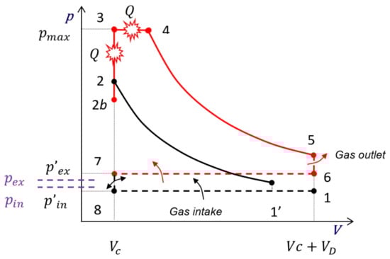
Figure 1.
Dual open cycle in a p-V diagram. Black lines show unburned gas, while red lines show burned gas. Continuous lines show closed processes, and dashed lines show cylinder open processes.
The present model incorporates all these effects as it considers an isobaric open process 8-1, shown in Figure 1. This makes the present model fill one of the gaps in the open literature.
1.4. Article Organization
Section 2 describes the main concepts in the model, highlighting the simplifying hypothesis. There, an expression for the end of intake gas temperature T1′ is developed, showing the need of calculating the previous cycle residual gas mass fraction f and its temperature Tr. This section also develops the theoretical and actual exhaust temperatures Tex, and Tex,ac as a function of the exhaust backpressure, pex, which is controlled by the exhaust cleaning devices, exhaust pipe, and the eventual turbocharging turbine.
Section 3 develops the cycle inner processes, from intake to exhaust, giving the thermodynamic state functions. It continues providing the explicit expressions of useful work W. A compatibility equation with the amount of fuel determines the heat released, Q. Both parameters allow us to obtain an explicit expression for the cycle efficiency, η. Having solved the cycle, expressions for the residual gas temperature, Tr, and residual gas mass fraction, f, close this section.
Section 4 performs some illustrative parametric variations. It starts with the simplest application of the model, using constant a priori fixed values for γ and mm and neglecting mass change in the closed part of the cycle internal processes. It continues revealing the effect of compression ratio and combustion pressure ratio , especially when there is a composition change, γ ≠ γb because of fuel–air ratio F > 0. The classical effect of cutoff ratio β is offered afterward. An analysis of alternatives for partializing load follows in that section, showing the superiority of unequal-strokes operation (r > re). The full expansion ratio Atkinson cycle is determined and its merits are discussed afterward. This section, as a checkpoint, compares the model expressions with simpler models, reaching the same results.
Within Section 4, Section 4.2 introduces variable properties results, highlighting the effect of the relative fuel-air ratio Fr. A discussion for reaching the maximum allowed pressure, pmax, closes this section.
Section 5 concludes by resuming the paper contributions and novelties, highlighting the model’s simplicity and flexibility.
2. Materials and Methods
The proposed open Dual cycle is a 0-dimensional model following a cyclic evolution in a p-V diagram for four-stroke engines. It is based on the following assumptions.
Working gases are ideal mixtures of non-reacting ideal gases with constant properties although process average temperatures determine their thermal properties, and . The trapped mass, m, is a mixture of air and, in due case, indirectly injected fuel (before Intake Valve Closing IVC), EGR, and residual gases from the previous cycle, such that its proportion is defined as f ≐ mr/m.
At TDC, the volume is minimum Vc. Adding the engine displacement VD, we obtain the maximum volume V1 = V7 at BDC. Figure 1 shows that compression starts when IVC, at an intermediate point 1′. These define the effective compression ratio re ≤ r (see Equation (3)).
When valves are open, the flow through them suffers stagnation pressure losses so that inside the cylinder, pressures are p′in and p′ex different to the pressures at the intake and exhaust pipes, pin and pex, Figure 1. Properties of trapped gas inside the cylinder, before combustion, have no indicating subscript, such as γ, cp, n, Rg, etc. These magnitudes have a “b” subscript (burned) after combustion to highlight the composition change.
External ram-effect in the intake collector, at the tuning speed, instantaneously increases the intake pressure pin isentropically up to p1′ at V = V1′ corresponding to IVC, by acoustic wave action, if considered in the engine design. πu = p1′/p′in > 1 empirically evaluates this phenomenon. πu ≈ 1.15 seems an upper boundary.
Internal compression from point 1′ to TDC (point 2) proceeds, either isentropically with constant γ or irreversibly with an equivalent polytrophic exponent n besides no mass losses, Figure 1. The imposed constant polytrophic efficiency of the compression process η∞,1′-2 allows us to calculate n. Polytrophic efficiency is considered a better option than isentropic efficiency as it is constant for any pressure ratio, Wilson and Korakianitis [24] with constant elementary efficiency η∞ (see Equation (4)).
This considers either heat gain or internal degradation, and heat transfer from/to the walls. Heat gain or internal irreversibility corresponds to n > γ or the equivalent 0 < η∞,1′-2 < 1. Heat loss corresponds to 0 < n < γ or the equivalent η∞,1′-2 > 1. The strange case of cooling beyond the initial temperature (temperature decrease) would correspond to n < 1; η∞,1′-2 < 0. In what follows, γ is retained, but if required it can be replaced by n on the exponent of Equation (10) and those continuing. This would be convenient for simulating a cold engine. With a mixture of non-reacting ideal gases, γ is a function of temperature, so that an intermediate estimated temperature between start and end of compression can be taken for a γ constant average value. A linear relation approximates the dependence of γ with temperature and composition for IC engines, such as the one proposed in Appendix C. In conventional engines running hot, the heat gain from the walls at the beginning of compression is in part compensated by heat loss at the later stages, so that an overall isentropic process is valid.
The location of the composition change during combustion (points 2 to 4 in Figure 1) does not affect the result of cycle performance, as (i) work is based on the integration of pdV and (ii) heat released to the gases is based on the amount of fuel burned when reaching point 4. This concept helps in obtaining analytical results and it is described in what follows.
Specifying the combustion initial state and the gas thermal properties at point 2 in the cycle, mass and energy balances, and the ideal gas equation, allows us to determine V4, T4, and m4, with specified gas properties after combustion, namely mm,b, γb, and p4. Instead of this single-pass calculation, three successive processes are considered: composition change 2-2b, constant volume 2b-3, and constant pressure 3–4 heat releases, to reach the same point 4, Figure 1. This allows us a better insight into the processes. This way, there is a correct systematic evaluation of the evolution between points 2 and 4, in terms of initial and final thermodynamic states, total work obtained, and total heat release. About the intermediate fictitious point, 2b, the only caution is to keep in mind that p2,b, and T2,b are not real but a convenient intermediate point for calculations.
At TDC, the composition change, due to combustion, is introduced in the model through the commented fictitious point, 2b, in an instantaneous single step, from unburned to burned gas mixture. This is equivalent to a step from n and γ to nb and γb respectively, along the constant volume process 2-2b in Figure 1. As stated in the previous paragraph this generates no error as processes from points 2 to 4 in Figure 1 do not use n, γ, nb nor γb in the calculations. From points 2 to 2b, there is still no heat release nor work so that internal thermal energy must be constant, here neglecting the enthalpy of the directly injected fuel. This allows us to calculate T2,b, and p2,b just by adding a mass balance and the ideal gas relations, as seen in Equation (5).
The proposed correlations in Appendix C allow us to calculate the changes in mm and γ for current fuels.
Both γ and γb depend on temperature so that considering average values between the corresponding cycle points, the issue of variable specific heats can be included approximately. γ can be shared by the one used in compression, which can be calculated at an estimated average temperature between the start and the end of compression (T1′ + T2)/2. With the same idea, (T3 + T4)/2 determines γb. A priori values of γ and γb allow us to approximate T2 and T4, respectively. Al-Sarki et al. [25,26] used a high-accuracy approximation to variable gas properties, giving a convenient formulation of the temperature effect on specific heat ratio, but not including nor . The effect of the injected fuel sensible enthalpy is usually negligible. Latent enthalpy, if not included in LHV, can be considered, if desired, by including the factor [1 + C F hfv/(cvT2)] in the temperature and pressure ratios in Equation (5). This detail is not included in the present paper as it focuses on the most impacting combustion effect on thermal properties.
After compression and composition change 2-2b, the lower heating value of the fuel LHV is released, along with the Dual combustion, process 2b-3-4 in Figure 1. In a real engine, some fuel remains unburned or burns partially, so that an internal combustion efficiency is considered ηcom,int, e.g., Heywood [2]. In our case, it includes the heat absorbed by dissociation.
In a normally operating engine, heat loss to the walls is highest during the combustion process of the cycle, owing to the high gas temperatures, density, and turbulence, so that another reducing factor Jcom includes this effect, such as in Hou [12]. It is current practice to consider a heat loss proportional to the average temperature during combustion (see Equation (26)). This allows us to perform optimizations of efficiency and work by varying basic cycle parameters, such as the compression ratio. Zao and Chen [27] and Ge et al. [28] give recent and comprehensive reviews on this class of models.
Following the classical Dual cycle model, combustion develops at constant TDC volume until the maximum pressure, pmax, is eventually reached. If this happens, then, combustion continues to maintain this pressure until all the fuel releases its heat. Pressure ratio α = p4/p2 ≥ 1 and the cutoff ratio β = V4/Vc ≥ 1 specify the shape of combustion, Figure 1. They are linked to maximum pressure and amount of burned fuel in Section 3 (see Equation (27)).
Expansion of burned gases proceeds with constant mass and no reaction down to BDC with the option of including an expansion polytrophic efficiency η∞,4–5 (see Equation (6)).
Heat loss corresponds to nb > γb or the equivalent η∞,4–5 > 1. Heat gain, internal mechanical dissipation, or heat release, correspond to nb < γb or the equivalent η∞,4–5 < 1.
As commented for γ during the compression stroke, γb is retained in what follows instead of nb, since burned gas expansion, with correctly operating conventional engines, can be approximately described by an isentropic process with specified initial and final volumes. This is widely recognized, e.g., by Taylor [3] and Heywood [2], among others. In real engines, the partial balance between heat release by residual combustion jointly with species recombination and heat loss to cylinder walls near TDC can explain this phenomenon.
Here, the presence of vestigial unburned gases, at the end of combustion, is neglected for properties changes.
A constant volume blowdown process happens spontaneously, 5–6. As a result of gas discharge, the pressure in the cylinder reduces to p′ex, a slightly higher pressure than the one in the exhaust collector pex, owing to valve and pipe empirical pressure losses, which is an option to include. This pressure is kept constant in the cylinder during the exhaust stroke up to TDC, while the piston forces the residual gases to exit in the process 6–7.
At TDC, the exhaust valve closes, and the intake valve opens; a mixing process 7–8 occurs between residual gases and fresh gases from the intake manifold, formed by air and eventually fuel and EGR. Pressure in the cylinder changes instantly to p′in, at constant volume. Residual gases blow out of the cylinder or fresh gases enter the cylinder, except when intake to exhaust pressure ratio is unity, rin = p′in/p′ex = 1. Intake stroke 8-1-1′ allows us to reintroduce all the residual gases that eventually have left the cylinder to the intake manifold and, later, a mass of fresh gases enter the cylinder, min. p′in is slightly lower than the intake pressure pin, owing to viscous irreversibilities in valves and pipes. Having passed the BDC, the intake valve closes the cylinder at point 1′, with trapped mass, m.
The parameters defining the open part of the cycle are p′in, rin, fresh gases temperature Tin and properties of the fresh gases mm,in and γin. Tin is the result of external compression ∆Tc, intercooling ∆Tint, evaporation of indirectly injected fuel ∆Tev (C ≠ 1), heat transfer to the walls ∆Tht, and EGR ∆TEGR. All of them can be calculated explicitly, as seen in Equation (7). The result is frequently Tin ≈ Tatm.
A mass and energy balance for the variable size control volume (CV) inside the cylinder, with a mass exchange, according to Figure 2, determines the temperature of the mixture at point 1′, see Equation (8). Moreover, Δm indicates the mass increment due to the pulse pressure ratio , corresponding to the external ram-effect at the tuning speed. Vu is the volume occupied by Δm inside the cylinder. The friction losses were neglected for the calculation of the intake enthalpy of that pulse. Residual gases properties are denoted with an “r” subscript (cv,r, and γr), instead of the burned “b” subscript, because the temperature of the residual gases is significantly lower than the average value used for the burned gases expansion, although can be assumed for the molar mass. considers that the inlet process occurs in two succesive phases, firstly at during inlet stroke and secondly at amounting , as a result of the pressure step driven by wave action.
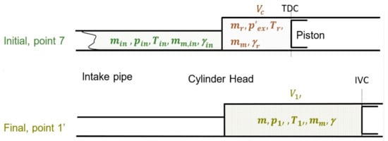
Figure 2.
Initial and final states of the intake process.
Below, Equation (31) shows that the temperature of residuals, Tr, is proportional to T1′; thus, an alternative expression to Equation (8) can be elaborated, as shown with Equation (9).
The cylinder residual gas mass fraction, f, is calculated below as part of the cycle, in Equation (11) or in a more elaborate fashion, in Equation (30). Specific heats cv are for either the mixture, residual, or intake of fresh gases. It can be calculated following Appendix A and Appendix C. Alternatively, the generally low value of f (normally some %) and a moderately low value of the fuel–air ratio make the approximation cv,r = cv = cv,in and γin = γ good enough for using Equations (8) and (9). The general effect of hot residuals is an increase of Tin in the range of 5 to 30 K.
The mass of fuel inside the cylinder mf is determined in Equation (10), considering that a fraction of the intake of fresh gases f is residual gas. The parameter EGR, typically < 0.3, quantifies the external recirculation level. Moreover, 0 ≤ C ≤ 1 is the fraction of the total fuel that is directly injected into the cylinder, assumed at the end of compression. The remaining is injected into the intake manifold or intake port.
Note: (in case is given referred to air mass).
The blowdown and forced exhaust 5-6-7 to a constant external pressure pex in the exhaust collector, upstream of the turbocharging turbine, determines the theoretical exhaust temperature Tex. Using Figure 3, mass and energy balances apply considering Vex as the total volume of the gases in the exhaust manifold, for both EGR and toward the turbine. They allow us to calculate the residual mass that remains in the cylinder mr. In Equation (11), γr ≥ γb is allowed because of lower temperatures, not affecting the cycle calculations.
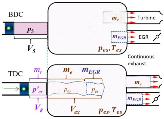
Figure 3.
Control volumes and variables during the exhaust process. Above, initial; below, final.
Equation (12) reduces to what is deduced in Ferguson and Kirkpatrick [5] for υ = 1, γ = γr, and mb = m. Equation (12) formulates a CM energy balance between initial and final states, points 5–7. The mass contained in the cylinder at point 6 is approximately proportional to mr and not to mb (m6 ~ rmr). As the process from 5 to 6 is too fast to be relevant regarding heat transfer, the cooling, due to heat transfer to cylinder walls from state 5 on, is proportional to mr in Equation (12). The empirical value ν takes into account this proportionality.
Equations (12) and (13) allow us to calculate the exhaust temperature, Tex, in Equation (13).
The rightest expression in Equation (13) coincides with the well-known model in Taylor [3]. T5 and p5 are a result of the cycle, and pex depends on the permeability of the turbine. The actual exhaust temperature Tex,ac is a result of both oxidation of unburned gases in the exhaust manifold during blowdown, and heat transfer to the manifold walls. Two combustion efficiencies determine the increase in temperature, because of internal combustion, ηcom,int, excluding dissociation for accuracy, and at the exhaust manifold ηcomb,ext, jointly with an unburned gas heating value LHVun ≅ LHV. The cooling is modeled by a heat transfer Newton equation, using an average wall temperature TW, see Equation (14).
These effects are opposite and normally of the same order of magnitude so that ignoring both processes is acceptable in a simplified analysis. As guidance, the classical reference Taylor [3] gives experimental values. Ferguson [5] gives values of hex coming from the Woschni correlation. Woschni correlations serve also to calculate υ for Equation (12). The value seems suitable in conventional circumstances if a better recommendation is lacking.
3. Cycle Calculation
Once the intake and exhaust processes and the framework of the model are solved, the calculation of the state at the internal points is straight ahead. The cycle relies on the basic parameters r, re, α, β, rin, p′in, EGR, Tin, and the non-dimensional parameter LHVvηcom,int,vJcom/(RgT1′) that Equation (28) introduces. As it is shown below, α and β are dependent on Fr through the fuel compatibility equation, Equation (28), so that Fr could substitute one of them plus data on the fuel and air to determine Fs (Appendix D). Fr jointly with pmax can substitute both, α and β parameters. Equation (11) or, in a more elaborate fashion, Equation (30) links the residual mass fraction, f, to the basic parameters. Equation (8) links T1′ to the temperature of intake fresh gases supplied to the engine Tin and the basic parameters. Numerical data from fuel and air, Appendix C, must be added for γ, γb, Rg, and Rg,b, which are also dependent on the basic parameters.
As composition change happens only in transformation 2-2b the sub-index “T” will not be used any longer in the energy balances when following Equation (2).
Compression
Constant Volume Combustion
Constant Pressure Combustion
The maximum temperature of the cycle is T4, which could be a limit for re in combination with fuel–air ratio (e.g., see Ozsoysal [9]).
Expansion
The isentropic exponent for expansion is again γb. Accepting a different average temperature for γb than during combustion, a higher accuracy could be gained.
Exhaust Blowdown
The process inside the cylinder is an isentropic expansion with γb, at constant volume and with mass outflow. Outside the cylinder, the expansion is irreversible, but this is irrelevant for cycle calculations. Choosing a higher value γr > γb because of the lower temperature would increase accuracy.
Exhaust Stroke
The process inside the cylinder is a volume displacement at constant pressure with mass outflow. υ considers heat losses.
The residual gases are at temperature Tr, as shown in Equation (12).
TDC Mixing
As the intake valve opens, the cylinder pressure equals the intake pressure with a mass interchange with the intake manifold. T8 would correspond to an isentropic expansion if rin > 1 and would correspond to a compression with some irreversibility at the intake valve if rin < 1. It is not modeled as it is not needed for calculating the cycle.
Intake Stroke
The cylinder pressure is constant up to IVC where a jump in pressure, πu, can happen, due to intake manifold tuning for positive action of acoustic pressure waves and non-steady ram effect.
Cycle Performances
Collecting all the contributions to work and with the help of Equation (23), we arrive at an expression either including the low-pressure loop (net work) or not (gross work). rin = 1.0 will be considered for gross work, which is indicated as the alternative option with brackets as subindex, as in Equation (22).
The definition of the mean effective pressure, mep, following Heywood [2], incorporates two alternatives, net and gross (see Equation (24)).
Considering Equation (23) mep results proportional to p1′, thus justifying supercharging, as well as intake wave action. In conventional spark-ignition engines, such as petrol engines, throttling reduces p′in, which implies reducing rin. This produces partial load, meaning a lower mep without needing to reduce F. In Equation (23), the influence of Tin is not explicit on the obtained expression for mep. Its influence comes through T1′, which is explicit in Equation (28).
Collecting heat released in 2b-3 and 3–4 processes gives the total heat released in the cycle, as in Equation (25).
Compatibility with the Fuel
In internal combustion engines, the fuel causes the internal heat release, as in Equation (26).
LHVv is the lower heating value of the fuel at constant volume, in the range of 40 to 55 MJ/kg for hydrocarbons, Taylor [3] and Heywood [2]. For many fuels, LHVv is close to the corresponding value at constant pressure LHV, as explained in Appendix B; but for future synthetic fuels, there can be a sensible difference. LHV is the common value used as a reference. For lean combustion and hot engine, normally the combustion efficiency ηcom,int,v < 1 can be close to 1.0, especially for compact combustion chambers and even more for stratified combustion. It falls for near rich lean mixtures and rich mixtures, as there is not enough oxygen for complete combustion (e.g., see Heywood [2] and Zerom and Gonca [19]).
Jcom considers the heat losses to the walls during the 2b-3 and 3–4 processes. In these processes, the losses are at the largest rate. During the other processes of the cycle, the heat flux is much lower (e.g., see Heywood [2] and Hou [12]). Therefore, the present study assumes that a net heat loss through the cylinder walls occurs only during combustion, excepting when n ≠ γ and/or nb ≠ γb are considered, as this implies heat transfer and/or heat release. The value of Jcom depends on the operating parameters of the engine, mainly it depends on the difference between gas and wall average temperatures and turbulence intensity, besides engine speed as a time scale for heat transfer. Representative values can be in the range of 0.8 to 0.9, although some authors indicate lower values, such as for Otto cycle in Mozurkewich and Berry [29,30], reported in Zhao and Chen [27], although this time for a Diesel cycle. These recommended values for Jcom could be judged as surprisingly high at a first sight, as heat rejection to coolant amounts typically from 0.2 to 0.4 of LHV. However, one must consider that a significant part of heat rejection to cylinder walls occurs during the exhaust blow-down and forced exhaust processes. Moreover, this loss includes external walls, such as exhaust valves, ports, and manifold, thus not affecting cycle calculations, which deals with internal processes, but contributing to heat rejection to the cooling circuit.
Numerous studies on cycles that are based on finite-time thermodynamics consider for Jcom something like what is considered here: an empirical temperature increase during combustion as a net result of heat release and heat loss to walls so that a linear relationship is accepted; for examples, see Klein [31] and Chen et al. [21,22], which offer, for an Otto cycle, the following relation, Equation (26), and Osman [32] for both cycles.
Hou [12] offers an equivalent expression for Dual cycles. This kind of relation accepts a heat loss proportional to average temperature during combustion, allowing for a variety of optimization procedures, e.g., Hou [11], Chen et al. [21,22], and Lin et al. [33]. The present model could incorporate this refinement, offering more accurate models, although the optimization analyses are beyond the scope of this paper.
Alternatively, other studies consider that during combustion, a fraction of LHV is lost by heat transfer to the walls Osman and Ozsoysal [32]. This fraction tends to be higher than the values for Jcom here recommended. The reason is that, in those studies, the compatibility between the increase in gas temperature during combustion and LHV is performed without considering combustion efficiency or composition change, as Equation (26) shows, with both reducing the end of combustion temperature.
Qcycle in Equation (24) must coincide with the net heat released by the fuel burning, Equation (26). From this, a compatibility condition arises, as seen in Equation (28).
Equation (28) indicates that both α and β increase with fuel-air ratio F, which is the independent variable. It also indicates that both decrease when T1′ increases, which is coherent.
For the Dual cycle, this equation allows us to explicitly solve for β imposing α = αmax, which is an input parameter equivalent to pmax/p2. The correct answer will be with β ≥ 1.0. If the solution yields β < 1.0 this means that all the combustion can be fully developed with V = const., without reaching pmax. For this case β = 1.0 should be imposed and Equation (28) explicitly solved for α. In a real engine, pmax is a result of the combustion development and because of that, it must be specified, using external information.
Net or gross fuel conversion efficiency takes into consideration the fuel delivered, according to Heywood [2]. Besides this, still, there are two possibilities (see Equation (29)).
This efficiency expression, using Equation (26), results in being only dependent on the basic parameters of the cycle, namely , and evantually . According to Appendix C, the properties dependency is and , where and depend again on the cycle basic parameters plus the inlet and exhaust thermodynamic states. can be considered an independent variable or depend the same way. is an external parameter. This results in a model that allows for more accurate, but simple, optimization studies.
To calculate the efficiency of the cycle alone, effective heat is the energy supplied to it. Thus the actual values of ηcom,vJcom have to be used to obtain Qcycle delivered to the cycle. If the engine efficiency is searched for, all the heat contained in the fuel is considered as supply, so that LHV has to be accounted for, as the energy delivered to the engine. Substitution of Equations (23) and (25) into Equation (29) results in an explicit expression for efficiency that is only dependent on the basic non-dimensional parameters r, re, rin, α, β, γ, and γb (and, eventually, n and nb if polytrophic evolutions are used, instead of isentropic, respectively, in the compression and expansion strokes.
T1′ in Equation (28) and elsewhere requires knowing the residual mass fraction f. Equation (11) can be elaborated into Equation (30).
This provides f as an explicit function if α and β are used as parameters for the cycle. If instead, the parameters are F and pmax/p2, Equation (28) has to be used, and obtaining f becomes implicit. A preliminarily estimated value for f allows us to start the cycle, providing an estimated T1′ through Equations (7) or (8), as the sensitivity to this parameter is low because f is in the order of 10−2 up to 10−1 for low rin. A better iterative approximation after cycle calculation can be obtained, as accurate as desired through subsequent iterations.
Taking into account the relations obtained in Section 3, it is possible to develop a compact expression for T5, and p5, by collecting the results of the cycle analysis; and from them, Tr for γb = γr, Equation (31). Equation (A7) allows us to calculate Rg/Rg,b.
These expressions, with approximate parameters, can also be used to start the cycle. As an example of procedure starting with a given value of F, we have the following: (i) Equation (30) can be used to estimate f, good enough to start iterating; (ii) with this value, Equation (7) or (8) provides T1′ and Equation (13) provides Tex for a given pex; (iii) α and β can be estimated from Equation (28) and a given pmax. For initial iterations, T1′ ≅ Tin + 30 K in a conventional engine operating normally, γ ≅ 1.38, γb ≅ γr ≅ 1.3, and (Rg/Rg,b) ≅ 1. In this example p′ex and Tin are considered data, but also can be iterated if matching of a turbocharger with the ICE is pursued, in case it is present.
4. Results
This section performs a parametric study, for illustrating the model performance predictions, at first simplifying to compare with simpler models, and then continuing to show full model results.
4.1. Constant Properties
This subsection considers γ and γb as constants; thus, they do not change with the basic parameters. This simplification allows for a fruitful, although limited, analysis and allows for non-iterative calculations.
Effect of Compression Ratio and Combustion Pressure Ratio
Figure 4 shows the effect of the variation of the compression ratio, r, when keeping constant all the other basic parameters for the case of constant volume heat release cycles; thus, β = 1. For cycles with γ = γb, one gets the well-known effect of a drop in efficiency for lower γ, bringing this figure of merit nearer to real values of ICEs. For these cases of γ = γb and β = 1.0, in Figure 4, the effect of pressure ratio α on the efficiency is negligible. For them, Equation (32) can be obtained, combining Equations (23), (25), and (29). The term correcting the Otto air standard cycle is small for rin ≈ 1.0 and re/r ≈ 1.0, and additionally, α being not too close to 1.0.
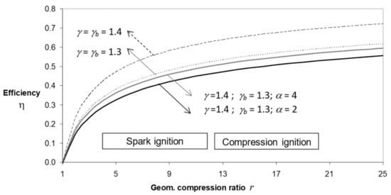
Figure 4.
Effect of compression ratio and γ on cycles with constant γ and γb, β = 1.0 (constant volume heat release) and rin = 1.0. re = 0.85r. Dashed lines correspond to cycles with γ = γb, valid for α = 2 to 4. Typical ranges for r are shown for both types of engines.
The scenario changes for γ ≠ γb. Figure 4. shows an example with γ = 1.4, grossly representative for unburned fuel–air mixtures. With γb = 1.3, grossly representative of burned gases, a drop in η is noticeable for lower values of α Although this drop is not too large, now the effect of α on the efficiency becomes substantial. The drop in efficiency becomes higher for lower α. This does not match reality. On the contrary, in a real engine, a lower α corresponds to a lower F, Equation (28), which results in higher efficiency. The reason for this discrepancy can be found in the lower temperatures of lean mixture combustion jointly with the resulting lower concentrations of CO2 and H2O, leading both separately to higher values for γb. Section 4.2 of this work shows that linking γb to F recovers all the physics of the problem and gives a higher efficiency for lower F. This highlights the capabilities of the proposed cycle model.
Effect of Cutoff Ratio β
The classical effect of β on efficiency can be easily revealed if again we assume γ = γb and for simplifying purposes we add the condition of r = re, rin = 1.0 and α = 1.0 so that the air-standard Diesel cycle is obtained. Then, from Equations (23), (25), and (29), we have Equation (33).
This equation for Diesel cycle efficiency differs from the one for the Otto cycle, Equation (1) by the factor indicated with *. This factor is >1.0 for normal values of β > 1.0 so that a lower efficiency is the result, and the difference is larger as β increases, with this meaning a higher load in a Diesel cycle. Equation (33) also indicates that pure constant pressure combustion is less efficient than pure constant volume combustion, but with the advantage of lower pressures and temperatures. The full equations, Equations (23), (25), and (29), also show this well-known phenomenon. They add the fact that decreasing β increases γb because of a lower F and lower temperature, which yields a higher increase in η.
Effect of Partial Load
In compression ignition engines (Diesel) reducing Fr reduces mep, thus reducing work per cycle or equivalently, torque; namely load, resulting in a two-fold increase in cycle efficiency. Firstly because of a reduction in β and secondly because of an increase in γb, predominant even when β = 1 and further Fr reductions diminish the value of α. Section 4.2 of this work shows this in detail. Unfortunately, homogeneous lean mixtures are difficult to ignite and burn completely, so that advanced spark-ignition engines (petrol) currently use alternative methods such as stratified combustion, HCCI (Homogeneous Charge Compression Ignition), or prechamber torch ignition.
When throttling is used to reduce load, rin diminishes, and a negative area low-pressure loop results in the cycle, as Figure 1 shows. This is because p′in < p′ex, leading to a drop in the cycle net efficiency η. A better practice uses a late intake valve closing (LIVC), using rin = 1.0, but r staying constant. This configures an Atkinson cycle, Benajes et al. [20], but more appropriately a Miller cycle, originally Miller [17] if turbocharging and intercooling is implemented. Figure 5 depicts the effect of diminishing load on both alternatives. The LIVC alternative yields a higher net efficiency at smaller than full load mep. Figure 6 depicts the ratio of both efficiencies, showing that the gain is higher when reducing mep and for low values of α and β. Non-constant gas properties further refine the results, but this does not modify the essentials.
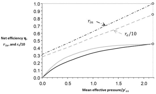
Figure 5.
Effect on efficiency of alternative methods of partializing load for cycles with constant γ and γb. Conventional throttling (reducing rin but r and re = cnt.), indicated with black lines, and LIVC (reducing re but r and rin = cnt.) indicated with gray lines. Full load corresponds to both rin = 1.0 and re = 8.5, yielding mep/p′ex = 2.18, as indicated. ηcom,int,v = 0.95; Jcom = 0.9; r = 10.0; α = 1.5; β = 1.0; γ = 1.4; γb = 1.3.

Figure 6.
The ratio of net efficiency for partial load cycles reducing re ≤ r = 8.5 over reducing rin ≤ 1.0, for the same mean effective pressure and cycles with constant γ and γb. Continuous lines are for α = 1.5, and dash lines for α = 3.0. Black lines are for β = 1.0, and gray lines for β = 2.0. The remaining parameters are of the same value as in Figure 5.
Optimum Expansion Ratio, rop
The commonly named geometric compression ratio r is the expansion ratio by which work is obtained. In an Atkinson/Miller cycle, re ≤ r. When r increases, keeping constant re, efficiency increases up to the optimum point, r = rop, when gas pressure at the end of expansion equals exhaust pressure, p5 = p′ex. Equation (34) allows us to calculate this optimum condition directly, using Equations (23), (25), and (29), and with γb corresponding to a lower average temperature because of the further expansion, if accuracy is pursued.
An engine with rop follows a full expansion Atkinson cycle. Unfortunately, rop depends on F through α and β, and it depends also on rin. As a result, it is dependent on the operating parameters. This implies that choosing it as a constant by an innovative kinematic crank mechanism of an enlarged expansion stroke seems not flexible enough. Moreover, what is more limiting, it can be up to around three times re, what makes that an Atkinson engine running with an effective compression ratio re not reduced by LIVC resulting too large and heavy for the same specific work obtained. Moreover, the piston friction of such a large expansion stroke will reduce the otherwise work gain. Using a turbine for completing the expansion externally seems a wise alternative, nowadays used for turbocharging.
The values of r given by current reciprocating engine designs can be near rop if re is small enough. These low values can be reached because of using LIVC for load reduction in a Miller cycle. Besides NOx considerations, this is one of the reasons that drive this strategy, jointly with variable IVC, on the present market for automotive engines.
4.2. Variable Properties
Both γ and γb are dependent on the respective average temperatures, as Section 2 indicates. Using data of Appendix C, and including equations for f and T1′ in a system of simultaneous equations (or by an iterative procedure), where cycle temperatures are calculated, higher accuracy is reached. Limitations up to now found because γ and γb being independent of basic parameters are no longer applying. Figure 7 shows the result of computing the efficiency against the geometric compression ratio r. Two fuel–air ratios are meaningful. Fr = 0.4 is representative of partial load. Fr = 0.9 is representative of full-load operation. This is so for engines that burn globally lean mixtures, such as the Diesel ones, and for lean mixture spark-ignition engines. Equation (28) gives the relation of α and β with Fr and through .
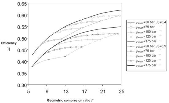
Figure 7.
The efficiency of the Dual Miller cycle vs. compression ratio for two fuel–air ratios (determining α and/or β) and five maximum pressures. , p′in = 2 bar, Tin = 300 K, EGR = 10%, rin = 1, ηcom,int,v = 0.95, Jcom = 0.9, re = 0.85r; γ and γb are dependent on temperature following the appendices. Both continuous lines with no markers show β = 1.0, for pressures below 175 bar (zone of intersection with symbol lines). Right side common boundary discontinuous lines show α = 1.0 and thus correspond to a pure Diesel cycle.
The results indicate that a leaner mixture yields higher efficiencies, which is coherent with reality, supporting the rationale of the preceding section. This removes the main limitation of air-standard cycles. Five maximum pressures were considered, covering representative values for both spark ignition (petrol) and compression ignition (Diesel) engines.
An increase in r results in higher efficiency, but with a pace that diminishes beyond the point where maximum cycle pressure pmax is reached, curves with symbols in Figure 7. This is the result of an increased fraction of constant pressure combustion, , beyond this point, in congruence with the comments made in the preceding section. The discontinuous lines defining the rightmost boundary limit of the curves with marks in Figure 7, correspond to , developing all the combustion at constant pressure (i.e., corresponding to a pure Diesel cycle). The continuous thick lines correspond to (pure Otto cycle) up to the point where the maximum pressure reaches the prescribed 175 bar limit. They show different efficiencies for the same compression ratio, showing the strong effect of Fr through , captured by the proposed model.
5. Conclusions
This study proposes a model of a Dual cycle with a single-step composition change, owing to internal combustion, and also includes gas exchange. It allows for the consideration of the effects of fuel with a simple and straightforward procedure. It includes advanced ICE features, such as EGR, residuals from the previous cycle, fuel composition, overexpansion, load reduction, Miller configuration, turbocharging, inlet inertial effect, and valves pressure losses. Large simplifications are obtained by considering an average temperature for the working gas properties at the cycle processes and the fuel–air ratio through a fuel compatibility condition, as seen in Equation (28). More specifically, we have the following:
- The composition change is performed at constant volume, just before combustion heat release. Thus, the change in mole number is included analytically through changes in γ and Rg. This way, the prediction of cycle performance is more realistic than with air-standard cycles. This is less cumbersome than with high-end computation tools and fuel-air cycles, but approaching its accuracy. In addition, the physics is retained within analytical expressions. These allow for easier predesign studies than those performed by means of computational tools.
- The obtained explicit performance formulae for the Dual Miller cycle are highly flexible and allow for the application of more accurate optimization procedures more simply than with fuel-air cycles. As an example, the analysis of partial load efficiency shows the advantages of including in the cycle model open processes for intake and exhaust.
- An explicit equation for the maximum cycle temperature yields the possibility to establish limiting conditions in optimization studies.
- A substantial effect on cycle performance of the change in γ to γb was found. The result is a more realistic figure for efficiency and a correct dependency on the fuel–air ratio. Appendix C of this paper offers unburned and burned gas thermal properties for variable fuel–air ratio cycle calculation, using simple correlations on the grounds of data given in the open literature.
- According to Figure 7, the effect of geometric compression ratio, r, with a constant fraction of heat losses, Jcom, shows that, after reaching the structurally acceptable maximum pressure, pmax, a further increase of compression ratio increases efficiency, but at a slower pace, as the combustion is displaced to the constant pressure zone that increases β, confirming classical results. The figure shows the ability of the proposed model to capture the strong effect of variations on γb due to Fr changes.
- The paper offers a straightforward explicit expression for the inlet temperature to the engine and to the turbocharging turbine, offering a more realistic background for further studies.
As for further works, a more detailed correlation for will be searched for. Including blow-by mass loss in a simple way could enhance the accuracy of the model. Data for renewable fuels and modified air (oxygen-enriched and/or N2 substituted by CO2) would extend the range of application of the model through simple correlations for the specific heat ratios.
Author Contributions
Conceptualization, A.L.; methodology, J.I.N., and A.F.; writing—original draft preparation, A.L.; writing—review and editing, A.L., J.I.N., and A.F. All authors have read and agreed to the published version of the manuscript.
Funding
This research received no external funding.
Institutional Review Board Statement
Not applicable.
Informed Consent Statement
Not applicable.
Data Availability Statement
No new data were created or analyzed in this study. Data sharing is not applicable to this article.
Conflicts of Interest
The authors declare no conflict of interest.
Abbreviations
| Symbol list | |
| bottom dead center | |
| constant | |
| Fuel-injected after compression/Total fuel = 1.0 for only in-cylinder fuel injection, 1 > C ≥ 0 otherwise | |
| number of carbon atoms in fuel molecule | |
| constant pressure and constant-volume specific heats [J kg−1 K−1) | |
| mass fraction of externally recirculated residuals | |
| mass fuel–air ratio | |
| relative fuel–air ratio = F/Fs | |
| mass fraction of residual gases from the previous cycle | |
| lower heat value of fuel at constant pressure (J kg−1) | |
| specific enthalpy (J kg−1) | |
| number of hydrogen atoms in fuel molecule | |
| heat transfer coefficient at the exhaust | |
| enthalpy of formation (J kg−1) | |
| fraction of lower heat value lost to walls | |
| Lower heating value | |
| mass (kg) | |
| mean effective pressure (Pa) | |
| molar mass (kg mol−1) | |
| number of moles | |
| polytrophic exponent | |
| pressure (Pa) | |
| maximum allowable pressure (Pa) | |
| heat (J) | |
| universal gas constant [8.314 J mol−1 K−1)] | |
| gas constant = R/mm [m2 s−2 K−1)] | |
| geometric compression ratio, expansion ratio: (Vc + VD)/Vc | |
| effective compression ratio: Vc/V1′ | |
| intake ratio: p′in/p′ex | |
| specific entropy [J kg−1 K−1)] | |
| temperature (K) | |
| internal energy (J) | |
| internal thermal energy (J) | |
| volume (m3) | |
| TDC volume (m3) | |
| displacement volume (m3) | |
| mechanical work, positive out of CM (J) | |
| mass fraction | |
| Greek | |
| α | pressure ratio during combustion = p4/p2 |
| β | cutoff ratio during combustion: V4/Vc |
| Δm | trapped mass increment due to intake pulse |
| γ | specific heats ratio |
| ηcom | combustion efficiency |
| η∞ | polytrophic efficiency |
| ν | ratio of residual to start of exhaust temperatures |
| σ | standard deviation |
| π | pressure ratio |
| Subscripts | |
| 0 | standard state |
| a | referred to air |
| ac | actual |
| atm | atmospheric |
| b | burned gases |
| c | charging compressor |
| c | number of carbon atoms |
| EGR | EGR |
| e | exhaust turbine |
| ex | exhaust burned gases |
| ev | fuel evaporation |
| f | fuel |
| fa | mixture of fuel and air |
| fv | fuel evaporation |
| Gross | no pumping losses |
| h | number of hydrogen atoms |
| ht | heat transfer |
| in | intake fresh gases |
| int | intercooling |
| o | number of oxygen atoms |
| r | residual burned gases |
| Net | Including pumping losses |
| q | chemical fraction of internal energy |
| s | stoichiometric fuel–air ratio |
| T | thermal fraction of internal energy |
| u | intake ram effect at tuning speed. |
| un | unburned. |
| v | constant volume |
| w | Exhaust manifold |
| Acronyms | |
| BDC | Bottom Dead Centre |
| CFD | Computational Fluid Dynamics |
| CM | Control Mass |
| CV | Control Volume |
| cnt. | constant |
| EGR | Exhaust Gas Recirculation |
| EGT | Exhaust Gas Temperature |
| EIVC | Early Intake Valve Closing |
| HCCI | Homogeneous Charge Compression Ignition |
| ICE | Internal Combustion Engine |
| IVC | Intake Valve Closing |
| LIVC | Late Intake valve Closing |
| TDC | Top Dead Center |
| ≐ | definition |
Appendix A
For an ideal mixture of I components of ideal gases, the specific heats follow Equation (A1).
Appendix B
Lower heat value at constant pressure and volume follow Equation (A2).
is the standard state temperature corresponding to , typically 298 K.
Appendix C
The effect of the specific heat ratio was determined as being important by Al-Saskhi et al. [25]; however, the precise values for the wide operating range in ICEs are challenging, as determined by Jarungthammachote [14]. Some authors have delivered correlations for both and against by using species chemical equilibrium, or frozen composition, for the latter, with as a parameter, as different formulations. Pressure effect is frequently not included for burned gas (e.g., see Ceviz and Kaymaz [34]), which is referred to in Wu et al. [35] as a simplified form. Pressure reduces dissociation for , which induces a change in , Heywood [2], which includes data for . Shehata [36] is a recent study on obtaining the polytropic exponent n. It shows a comparison of the experimentally obtained values with different correlations for and , such as Brunt et al. [37] Gatowski et al. [38], and Klein [39]. The following simple correlations offer a tool in concordance with these recently published data.
Unburned Gases
Considering that EGR and residuals have the same composition, a linear fit to data in Heywood [2] for air and petrol vapor yields Equation (A3).
Considering an ideal mixture for reactants, we obtain Equation (A4).
Burned Gases, Residuals, and EGR
A linear fit to data available in Heywood [2] for 300 K < T < 3000 K, isooctane and equilibrium species, are Equations (A5) and (A6). For hydrocarbons down to H2 and usual alcohols, they deviate less than 1%, so that a separate correlation is not necessary.
Gatowski et al. [38], Feng et al. [40] offer a correlation with a joint temperature and fuel–air ratio dependency coherent with Equations (A5) and (A6).
With Equations (A5) and (A6), at Fr = 1.0 (stoichiometry), there is a jump in γb < 2.5%. It should not be surprising that, for lean mixtures, the sensitivity of γ and γb to temperature is similar, as the main constituent of the mixture is N2.
Considering the effect of h/c through product from composition for lean mixtures and considering the data offered in Heywood [2] for rich mixtures, the molar mass of burned hydrocarbon/air gases can be approximated by Equation (A7).
For H2, the h/c = 4 can be used with no appreciable loss of the model accuracy.
Appendix D
For a fuel composition of CcHhOo and air molar composition of O2 + 3.714N2 + 0.047Ar, the stoichiometric fuel–air ratio is given by Equation (A8).
References
- Moran, M.J.; Shapiro, H.N.; Boettner, D.D.; Bailey, M.B. Fundamentals of Engineering Thermodynamics, 9th ed.; Wiley: New York, NY, USA, 2018; ISBN 9781119391388. [Google Scholar]
- Heywood, J. Internal Combustion Engine Fundamentals; McGraw-Hill: New York, NY, USA, 1988; ISBN 007028637-X. [Google Scholar]
- Taylor, C.F.; Glaister, E. The Internal Combustion Engine in Theory and Practice. J. Appl. Mech. 1961, 28, 316–317. [Google Scholar] [CrossRef][Green Version]
- Stone, R.S. Introduction to Internal Combustion Engines, 3rd ed.; SAE International: Warrendale, PA, USA, 1999; ISBN 0768004950. [Google Scholar]
- Ferguson, C.; Kirkpatrick, A.T. Internal Combustion Engines Applied Thermosciences, 2nd ed.; John Wiley & Sons, Inc.: Hoboken, NJ, USA, 2001; ISBN 978-0471356172. [Google Scholar]
- Ebrahimi, R. Effect of specific heat ratio on heat release analysis in a spark ignition engine. Sci. Iran. 2011, 18, 1231–1236. [Google Scholar] [CrossRef][Green Version]
- Zhao, Y.; Chen, J. Performance analysis of an irreversible Miller heat engine and its optimum criteria. Appl. Therm. Eng. 2007, 27, 2051–2058. [Google Scholar] [CrossRef]
- Ge, Y.; Chen, L.; Sun, F. Finite-time thermodynamic modelling and analysis for an irreversible Dual cycle. Math. Comput. Model 2009, 50, 101–108. [Google Scholar] [CrossRef]
- Ozsoysal, O.A. Effects of combustion efficiency on a Dual cycle. Energy Convers. Manag. 2009, 50, 2400–2406. [Google Scholar] [CrossRef]
- Wu, Z.; Chen, L.; Ge, Y.; Sun, F. Thermodynamic optimization for an air-standard irreversible Dual-Miller cycle with linearly variable specific heat ratio of working fluid. Int. J. Heat Mass Transf. 2018, 124, 46–57. [Google Scholar] [CrossRef]
- Hou, S.-S. Comparison of performances of air standard Atkinson and Otto cycles with heat transfer considerations. Energy Convers. Manag. 2007, 48, 1683–1690. [Google Scholar] [CrossRef]
- Hou, S.-S. Heat transfer effects on the performance of an air standard Dual cycle. Energy Convers. Manag. 2004, 45, 3003–3015. [Google Scholar] [CrossRef]
- Gordon, S.; Mcbride, B.J. Computer Program for Calculation of Complex Chemical Equilibrium Compositions and Applications. Part 1: Analysis; NASA Reference Publication (RP) 19950013764; NASA: Palo Alto, CA, USA, 1994.
- Jarungthammachote, S. Simplified model for estimations of combustion products, adiabatic flame temperature and properties of burned gas. Therm. Sci. Eng. Prog. 2020, 17, 100393. [Google Scholar] [CrossRef]
- Glassman, I. Combustion, 2nd ed.; Academic Press: Waltham, MA, USA, 1987; ISBN 0122858514. [Google Scholar]
- NASA. Chemical Equilibrium with Applications, NASA; 2002. Available online: https://www1.grc.nasa.gov/research-and-engineering/ceaweb/ (accessed on 2 May 2021).
- Miller, R.H. Supercharging and Internal Cooling Cycle for High Output; Trans ASME: San Francisco, CA, USA, 1947; Volume 69, pp. 453–457. [Google Scholar]
- Gonca, G. An Optimization Study on an Eco-Friendly Engine Cycle Named as Dual-Miller Cycle (DMC) for Marine Vehicles. Pol. Marit. Res. 2017, 24, 86–98. [Google Scholar] [CrossRef]
- Zerom, M.S.; Gonca, G. Multi-criteria performance analysis of dual miller cycle—Organic rankine cycle combined power plant. Energy Convers. Manag. 2020, 221, 113121. [Google Scholar] [CrossRef]
- Benajes, J.; Serrano, J.; Molina, S.; Novella, R. Potential of Atkinson cycle combined with EGR for pollutant control in a HD diesel engine. Energy Convers. Manag. 2009, 50, 174–183. [Google Scholar] [CrossRef]
- Chen, L.; Wu, C.; Sun, F.; Cao, S. Heat transfer effects on the net work output and efficiency characteristics for an air-standard Otto cycle. Energy Convers. Manag. 1998, 39, 643–648. [Google Scholar] [CrossRef]
- Chen, L.; Zeng, F.; Sun, F.; Wu, C. Heat-transfer effects on net work and/or power as functions of efficiency for air-standard diesel cycles. Energy 1996, 21, 1201–1205. [Google Scholar] [CrossRef]
- Luo, Q.-H.; Sun, B.-G. Effect of the Miller cycle on the performance of turbocharged hydrogen internal combustion engines. Energy Convers. Manag. 2016, 123, 209–217. [Google Scholar] [CrossRef]
- Wilson, D.G.; Korakianitis, T. The Design of High-Efficiency Turbomachinery and Gas Turbines, 2nd ed.; The MIT Press: Cambridge, MA, USA, 2014. [Google Scholar]
- Al-Sarkhi, A.; Al-Hinti, I.; Abu-Nada, E.; Akash, B. Performance evaluation of irreversible Miller engine under various specific heat models. Int. Commun. Heat Mass Transf. 2007, 34, 897–906. [Google Scholar] [CrossRef]
- Al-Sarkhi, A.; Jaber, J.; Abu-Qudais, M.; Probert, S. Effects of friction and temperature-dependent specific-heat of the working fluid on the performance of a Diesel-engine. Appl. Energy 2006, 83, 153–165. [Google Scholar] [CrossRef]
- Zhao, Y.; Chen, J. Optimum performance analysis of an irreversible Diesel heat engine affected by variable heat capacities of working fluid. Energy Conversion and Management. Energ. Convers. Manag. 2007, 48, 2595–2603. [Google Scholar] [CrossRef]
- Ge, Y.; Chen, L.; Sun, F.; Wu, C. Thermodynamic simulation of performance of an Otto cycle with heat transfer and variable specific heats of working fluid. Int. J. Therm. Sci. 2005, 44, 506–511. [Google Scholar] [CrossRef]
- Mozurkewich, M.; Berry, R.S. Optimal paths for thermodynamic systems: The ideal Otto cycle. J. Appl. Phys. 1982, 53, 34–42. [Google Scholar] [CrossRef]
- Mozurkewich, M.; Berry, R.S. Finite-time thermodynamics: Engine performance improved by optimized piston motion. Proc. Natl. Acad. Sci. USA 1981, 78, 1986–1988. [Google Scholar] [CrossRef] [PubMed]
- Klein, S.A. An Explanation for Observed Compression Ratios in Internal Combustion Engines. J. Eng. Gas. Turbines Power 1991, 113, 511–513. [Google Scholar] [CrossRef]
- Ozsoysal, O.A. Heat loss as a percentage of fuel’s energy in air standard Otto and Diesel cycles. Energy Convers. Manag. 2006, 47, 1051–1062. [Google Scholar] [CrossRef]
- Ge, Y.; Chen, L.; Sun, F. Finite-time thermodynamic performance of a Dual cycle. Int. J. Energ. Res. 1999, 23, 765–772. [Google Scholar] [CrossRef]
- Ceviz, M.; Kaymaz, I. Temperature and air–fuel ratio dependent specific heat ratio functions for lean burned and unburned mixture. Energy Convers. Manag. 2005, 46, 2387–2404. [Google Scholar] [CrossRef]
- Wu, Y.-Y.; Wang, J.H.; Mir, F.M. Improving the Thermal Efficiency of the Homogeneous Charge Compression Ignition Engine by Using Various Combustion Patterns. Energies 2018, 11, 3002. [Google Scholar] [CrossRef]
- Shehata, M.S. Cylinder pressure, performance parameters, heat release, specific heats ratio and duration of combustion for spark ignition engine. Energy 2010, 35, 4710–4725. [Google Scholar] [CrossRef]
- Brunt, M.F.; Rai, H.; Emtage, A.L. The Calculation of Heat Release Energy from Engine Cylinder Pressure Data; SAE Technical Paper 981052; Society of Automotive Engineering: Warrendale, PA, USA, 1998. [Google Scholar] [CrossRef]
- Gatowski, J.A.; Balles, E.N.; Chun, K.M.; Nelson, E.F.; Ekchian, J.A.; Heywood, J.B. Heat Release Analysis of Engine Pressure Data; SAE Technical Paper 841359; Society of Automotive Engineering: Warrendale, PA, USA, 1984. [Google Scholar] [CrossRef]
- Klein, M.A. Specific Heats Ratio Model and Compression Ratio Estimation. Thesis No. 1104, Linköping University, Linköping, Sweden, 2004. Available online: https://www.vehicular.isy.liu.se/Publications/Lic/04_LIC_1104_MK.pdf (accessed on 2 May 2021).
- Feng, Y.; Wang, H.; Gao, R.; Zhu, Y. A Zero-Dimensional Mixing Controlled Combustion Model for Real Time Performance Simulation of Marine Two-Stroke Diesel Engines. Energies 2019, 12, 2000. [Google Scholar] [CrossRef]
Publisher’s Note: MDPI stays neutral with regard to jurisdictional claims in published maps and institutional affiliations. |
© 2021 by the authors. Licensee MDPI, Basel, Switzerland. This article is an open access article distributed under the terms and conditions of the Creative Commons Attribution (CC BY) license (https://creativecommons.org/licenses/by/4.0/).