Article

Impact of Hydropower on Air Pollution and Economic Growth in China

1
School of Big Data Application and Economics, Guizhou University of Finance and Economics, Guiyang 550025, Guizhou, China
2
Green Development Strategy Research Institute (First Batch of New Characteristic Think Tanks in Guizhou), Guizhou University of Finance and Economics, Guiyang 550025, Guizhou, China
3
Department of Geography, The University of Hong Kong, Hong Kong 999077, China
*
Author to whom correspondence should be addressed.
Energies 2021, 14(10), 2812; https://doi.org/10.3390/en14102812
Submission received: 22 March 2021 / Revised: 30 April 2021 / Accepted: 7 May 2021 / Published: 13 May 2021

Abstract

:
The development of renewable clean energy such as hydropower can not only ensure energy security, but also help achieve the United Nation’s Sustainable Development Goals. This paper uses the annual data of 30 provinces in China from 2000 to 2017, and constructs a dynamic spatial Durbin model and a geographically weighted regression model to empirically test the dynamic impact of hydropower on haze pollution and economic growth at the national and provincial levels. The empirical results show that the promoting effect of hydropower on economic growth in Western China is less than that in Eastern China, which further aggravates the economic development gap between the eastern and western regions. In addition, the suppression effect of hydropower on the haze pollution in the western region is greater than that in the eastern region, where the haze pollution is serious. From the national level, hydropower can promote regional economic growth and inhibit haze pollution, and the spatial spillover effects of these two effects are greater than the local effects, and the long-term impact is greater than the short-term impact. The research conclusions of this paper will help China realize the sustainable development goals of energy saving and emission reduction.

1. Introduction

Since the Industrial Revolution, the rapid growth of the industrial economy has become the main driving force for the sustained growth of the world economy (Xu et al., 2019 [1]). However, industry belongs to high energy consumption and high pollution sector. Long-term economic growth driven by industrial economy will inevitably increase the consumption of fossil energy, which will promote the continuous increase in the emissions of carbon dioxide, sulfur dioxide and nitrogen oxides (Shao et al., 2017 [2]). This eventually leads to a series of problems such as air pollution and global warming. In order to ensure universal access to modern energy services and improve the efficiency and use of renewable energy, the UN proposed energy sustainability goals in 2015.
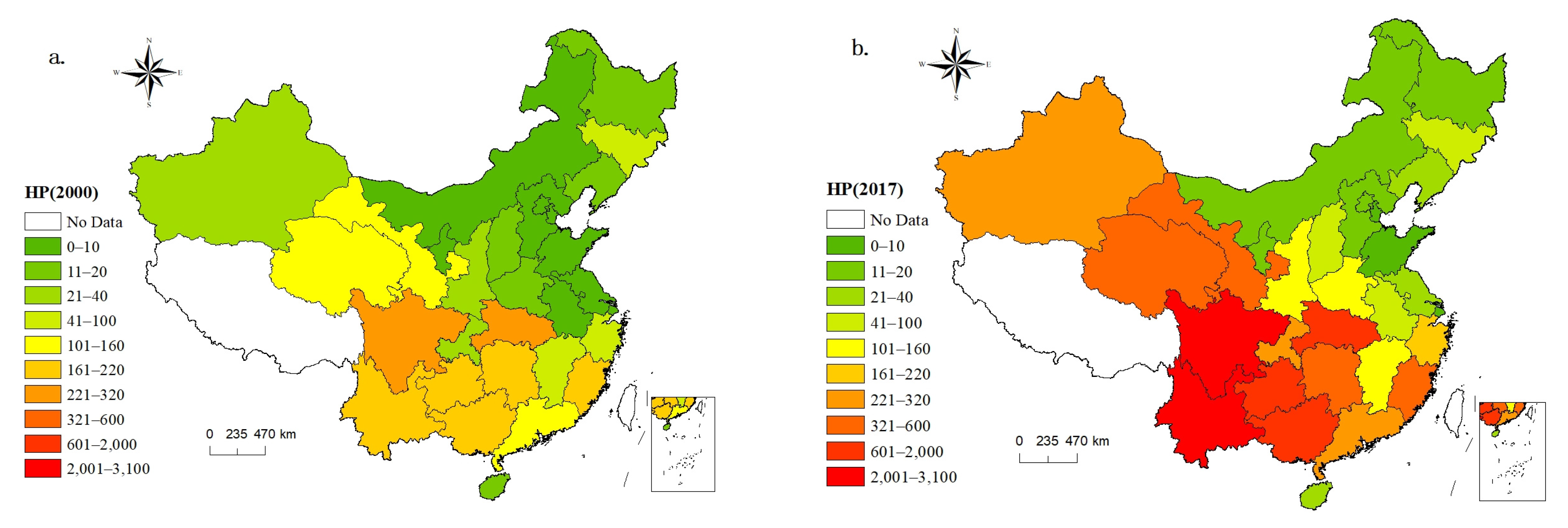
Energy sustainability is an important part of the UN’s Sustainable Development Goals. Since reforming and opening up, China’s economy has maintained a medium-to-high speed growth, and economic growth will inevitably lead to a large demand for resources. China’s energy structure is dominated by fossil energy. According to data from the Resset database, raw coal and crude oil accounted for 75.5% of total energy output in 2019. However, clean energy such as hydropower, nuclear power and wind power only accounted for 18.8% of total energy output. In recent years, the air pollution problem dominated by haze has seriously affected the quality of China’s economic growth, public health and government image (Chen and Chen, 2018 [3]; Yang et al., 2020 [4]; Anser et al., 2020 [5]). China’s haze pollution is increasing, and high-polluting areas gradually show the characteristics of spatial agglomeration, mainly concentrated in the Beijing-Tianjin-Hebei region, the Yangtze River Delta region and its adjacent central region, as well as three provinces in the northwestern region (Figure 1).
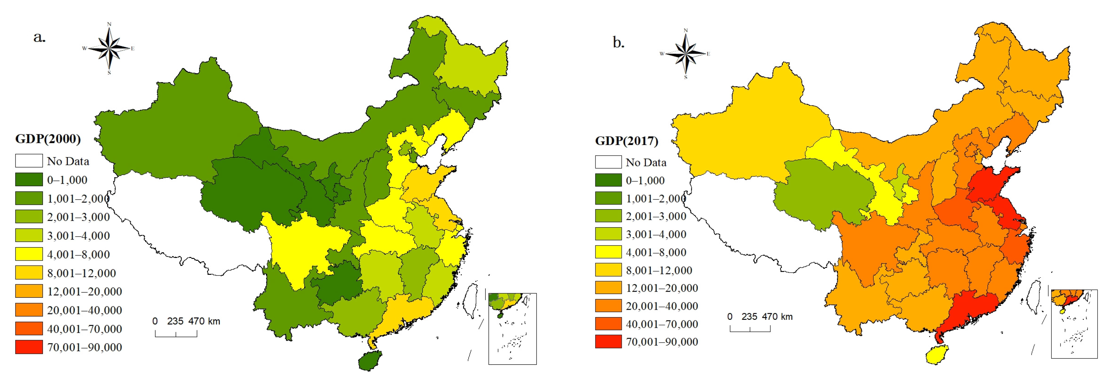
According to data from the China Energy Statistical Yearbook, China’s hydropower generation in 2017 was 1.188 billion kilowatt-hours (except Tibet, Hong Kong, Macau and Taiwan), which is 1.86 times that of nuclear, wind and solar power. The terrain of China is high in the west and low in the east, showing a three-step ladder distribution. The western region, especially the southwest region, is dominated by mountainous areas with a large topographic drop, which contains abundant hydropower resources. However, the eastern region is dominated by plains and hills, with little topographic fluctuation, which is not suitable for the development of hydropower resources. China’s hydropower generation has been increasing year by year, and it is mainly concentrated in southwest China and Hubei Province in central China (Figure 2). However, China’s economic distribution shows a pattern of high in the east and low in the west (Figure 3). The economic scale in the eastern region is large and the demand for power resources is large, while the economic scale in the western region is relatively small and the power resources are abundant. China’s energy resources and load centers are generally in a reverse distribution trend. In addition, China’s provincial hydropower, haze pollution and economic growth have the characteristics of spatial agglomeration, and there may be spatial spillover effect, that is, the regional hydropower has an impact on the haze pollution and economic growth of neighboring regions.
In order to promote the coordinated economic development of Eastern and Western China, realizing the optimal allocation of energy resources across China, China put forward the concept of the “West-to-East Power Transmission” project in the 1980s and began to implement it in the 1990s. The aim of the “West-to-East Power Transmission” is mainly to transform the abundant hydropower resources in the western region into power resources and transmit them to the eastern coastal areas where power is scarce. Due to the clean electricity substitution provided by hydropower, the consumption of standard coal in the China Southern Power Grid alone has been reduced by more than 100 million tons, and the emissions of carbon dioxide, sulfur dioxide, nitrogen oxides and other gases have been effectively reduced, providing important support for the realization of China’s energy conservation and emission reduction targets (Hu and He, 2014 [6]; Yu, 2020 [7]).
In the context of sustainable global energy development, the development of renewable clean energy can not only ensure energy security, but also achieve green and sustainable development. Hydropower resources account for most of China’s clean energy. Exploring the impact of hydropower resources on air pollution and economic development will help China achieve its sustainable development goals for energy conservation and emission reduction and promote its ecological civilization construction.
The marginal contribution of this paper is reflected in the following two aspects: (1) Based on the spatial perspective, the spatial econometric model is constructed to empirically test the spatial spillover effect of hydropower on haze pollution and economic growth; (2) Due to the inverse distribution of China’s economic scale and hydropower resources, this paper constructs a geographically weighted regression (GWR) model to test the spatial heterogeneity of the impact of hydropower on haze pollution and economic growth at regional and provincial scales.

2. Literature Review

Actively developing clean energy can not only meet the growing energy demand of economic growth and people’s lives, reduce carbon dioxide, sulfur dioxide and nitrogen oxide emissions, but also promote the transformation and upgrading of industrial structures and achieve high-quality economic development. Therefore, more and more scholars are beginning to pay attention to the development of clean energy, and to study whether clean energy can reduce polluting gas emissions and promote economic growth.
Research on the impact of developing clean energy on air quality. Based on the spatial perspective, some scholars believe that an effective way to reduce the PM2.5 concentration in areas with high concentration of haze pollution is to change the energy structure and increase the development and utilization of clean energy (Ma and Zhang, 2014 [8]; Li et al., 2020 [9]). Wei and Zhao (2017) [10] used the computable general equilibrium model to quantitatively study the positive effect of renewable energy price subsidy policies on improving air quality in China from the perspective of total volume and industry, and the results showed that renewable energy price subsidies reduced the total emissions of greenhouse gases and polluting gases. Xu (2018) [11] built a dynamic computable general equilibrium model to simulate that China’s clean energy subsidy policy can effectively improve the total output of energy, industry and other related industries, change the elasticity of substitution between fossil fuels and clean energy, and reduce the emission intensity of major pollutants. Xie et al. (2021) [12] found that the new energy subsidy policy can significantly reduce the current air pollution by using the Propensity Score Matching-Difference in Difference (PSM-DID) method. As for the effect of clean energy on carbon dioxide emission reduction, some scholars believe that there is a two-way causality between clean energy and carbon dioxide, and the active development of clean energy can effectively reduce carbon dioxide emission (Dogan and Seker, 2016 [13]; Zoundi, 2017 [14]; Razmjoo et al., 2020 [15]).
Research on the impact of developing clean energy on economic growth. Zhang and Liu (2015) [16] built a dynamic Overlapping Generation-Computable General Equilibrium (OLG-CGE) model and found that the development of clean energy could inhibit and promote economic growth through different mechanisms in the short and long term. Some scholars have found that clean energy development can effectively promote sustainable economic growth by empirical analysis (Inglesi-Lotz, 2016 [17]; Bhattacharya et al., 2016 [18]; Lin, 2017 [19]; Pilatowska et al., 2021 [20]). Kahia et al. (2017) [21] used Granger test and panel error correction model to conduct empirical research, and concluded that there was a two-way long-term and short-term causal relationship between economic growth and clean energy. Destek and Aslan (2017) [22] argued that when using the same model to examine the relationship between clean energy development and economic growth in different countries, the results were also significantly different. Keček et al. (2019) [23] used an input-output model to study the economic impact of the deployment and operation of renewable energy plants in Croatia, and the results showed that the deployment and operation of renewable energy plants have a positive product effect on economic growth. Xu et al. (2019) [1] used a non-parametric additive regression model to study the impact of clean energy development in China on regional economic growth. They found that, from a non-linear perspective, the impact of clean energy development on economic growth in the eastern, central and western regions is at different stages.
The existing literature provides useful references for the research of this article, but there are still areas for improvement. Firstly, China’s provincial hydropower generation, haze pollution and regional economic growth have spatial agglomeration characteristics and may have spatial spillover effects. If this spatial spillover effect is not considered, estimation bias may exist. In addition, the “West-to-East Power Transmission” project will transfer hydropower resources from the western region to the eastern region, which will undoubtedly enhance the spatial spillover effect of hydropower on the economic growth and haze pollution in the eastern region. Although Ma and Zhang (2014) [8] used spatial econometric models to empirically analyze the impact of energy structure on haze pollution from the overall level, they failed to fully analyze the impact of hydropower on haze pollution and economic growth. Secondly, the existing literature mostly studies the impact of clean energy on haze pollution and economic growth from the national level. China has a vast territory with a large span from east to west, and the distribution of hydropower resources in various regions is uneven. Due to historical reasons, the industrial structure, environmental pollution and economic development level of China’s eastern, central and western regions also differ greatly. If we ignore the regional differences in China, the conclusions obtained from research at the national level cannot be applied to the actual needs of various regions.
To address the above drawbacks, this paper selects the annual data of 30 provinces in China (except Tibet, Hong Kong, Macao and Taiwan) to build a spatial econometric model to empirically analyze the spatial spillover effect and local effect of hydropower on regional economic growth and haze pollution, and uses GWR Model to explore the spatial heterogeneity characteristics of the impact of hydropower on economic growth and haze pollution.

3. Methodology and Data

3.1. Spatial Correlation Analysis

The global Moran index I is used to test the global spatial auto-correlation of hydropower, economic growth and haze pollution in China’s provinces. The calculation formula is as follows:
I = i = 1 n j = 1 n w i j ( x i x ¯ ) ( x j x ¯ ) S 2 i = 1 n j = 1 n w i j
Among them, S 2 = 1 n i = 1 n ( x i x ¯ ) 2 is the sample variance. x ¯ = 1 n i = 1 n x i , x i is the amount of hydropower generation in province i or the actual GDP per capita or the value of haze concentration in province i . w i j is the spatial weight matrix. The Moran’s I index ranges from −1 to 1. When the index is greater than 0, it indicates that hydropower, economic growth or haze pollution in one province has a positive spatial auto-correlation; when the index is less than 0, it indicates that the provincial hydropower, economic growth or haze pollution has negative spatial auto-correlation; when the index is equal to 0, it indicates that there is no spatial auto-correlation, and its distribution is random.

3.2. Model Construction

3.2.1. Economic Growth Model

Most existing studies use the Solow growth model to analyze the factors that affect economic growth. Based on the Solow growth model and drawing on the research results of Lin and Sun (2011) [24], Xu et al. (2019) [1], this article sets the equation as:
Y t = A t K t α L t β
where Y is the output level, K is capital investment, L is labor input, α is the contribution ratio of capital input to output, β is the contribution ratio of labor input to output, the constant A is technological progress and t is the year. In addition, clean energy can not only optimize the energy structure, but also promote the optimization and upgrading of the industrial structure, thereby promoting green economic growth. Based on Equation (2), we introduce hydropower and other control variables, and take the logarithm to obtain Equation (3):
ln E G i t = β 0 + β 1 ln H P i t + β 2 ln R D i t + β 3 ln C S i t + β 4 ln E P i t + β 5 ln U R i t + β 6 W S i t + μ i t
where E G i t is regional economic growth, measured with real GDP per capita, H P i t is the amount of hydropower generation, R D i t is the internal expenditure of R&D funds, which measures technological progress from the perspective of R&D investment, C S i t is capital stock, E P i t is the number of employees, U R i t is urbanization, W S is water scarcity, β i is the coefficient of the explanatory variable and μ i t is the random error term.
We further explore whether there is spatial spillover effect between the development of clean energy and other social and economic activities, thus exerting an impact on the economic growth of surrounding areas; this paper constructs a spatial econometric model based on Equation (3):
ln E G i t = ρ W i j ln E G i t + β 1 ln H P i t + β 2 ln R D i t + β 3 ln C S i t + β 4 ln E P i t + β 5 ln U R i t + β 6 W S i t       + θ 1 W i j ln H P i t + θ 2 W i j ln R D i t + θ 3 W i j ln C S i t + θ 4 W i j ln E P i t + θ 5 W i j ln U R i t + θ 6 W i j W S i t       + α i + φ i + μ i t μ i t = δ W i j μ i t + ε i t
where ε i t N ( 0 , σ 2 I n ) , ρ is the spatial lag coefficient of economic growth, θ i is the spatial lag coefficient of the explanatory variable, W i j is the spatial weight matrix, δ is the spatial error coefficient and α i and φ i represent the space fixed effect and time fixed effect, respectively. The meaning of the remaining variables is the same as described above.

3.2.2. Haze Pollution Model

The STIRPAT (Stochastic Impacts by Regression on Population, Affluence and Technology) equation (Dietz and Rosa, 1997 [25]) was used to study the impact of population economic activities on environmental changes in most of the previous literature. Its expression is:
I i = a P i b A i c T i f e i
where I i is environmental pollution, P i is population size, A i is wealth per capita, T i is technology level and e i is random error term. In addition, Lin (2017) [19] confirmed that the energy structure significantly impacts haze pollution, and the development of clean energy can effectively reduce exhaust emissions, thereby improving air quality. In order to investigate the inhibitory effect of clean energy development on haze pollution, this paper uses the haze concentration (lnPM) to express the air pollution in the model. At the same time, drawing lessons from the research framework of the Environment Kuznets Curve (EKC) hypothesis, the primary and secondary terms of per capita regional GDP are included in the explanatory variables as the output level to measure whether there is an inverted “U” relationship between economic development and environmental pollution. Based on Equation (5), this article introduces industrial structure variables and takes the logarithm of both sides to obtain (Cheng, 2019 [26]; Gong, 2020 [27]):
ln P M i t = β 0 + β 1 ln H P i t + β 2 P D i t + β 3 ln E G i t + β 4 ( ln E G i t ) 2 + β 5 ln R D i t      + β 6 I S i t + β 7 W S i t + μ i t
where P D i t is the population density and ln E G i t and ( ln E G i t ) 2 are the primary and secondary terms of per capita output, respectively, used to measure the nonlinear relationship between economic growth and haze pollution. I S i t is the industrial structure. The meaning of the remaining variables is the same as previously described.
Haze pollution has a significant positive spatial auto-correlation, and social economic activities have spatial spillover effects on haze pollution (Shao, 2016) [28]. Therefore, based on Equation (6), we construct the following spatial econometric model to explore the spatial spillover effects of clean energy development and other variables on haze pollution:
ln P M i t = ρ W i j ln P M i t + β 1 ln H P i t + β 2 P D i t + β 3 ln E G i t + β 4 ( ln E G i t ) 2 + β 5 ln R D i t      + β 6 I S i t + β 7 W S i t + θ 1 W i j ln H P i t + θ 2 W i j P D i t + θ 3 W i j ln E G + θ 4 W i j ( ln E G i t ) 2      + θ 5 W i j ln R D i t + θ 6 W i j I S i t + θ 7 W i j W S i t + φ i + μ i t μ i t = δ W i j μ i t + ε i t
In Equation (7), the meaning of each variable is the same as above.

3.2.3. GWR Model Construction

The GWR model embeds the geographic location information of the sample points into the regression parameters, which can indicate that the results of the parameter estimation will vary along with the changes of geographic location. It can reflect the spatial non-stationarity of the research object (Brunsdon et al., 1996 [29]). The GWR model is constructed to explore the impact of spatial heterogeneity of hydroelectric power generation on regional haze pollution and economic growth. In this paper, the Gaussian function and the Akaike Information Criterion method are used to determine the optimal bandwidth (Xu and Lin, 2020 [30]).
Y i = α 0 ( u i , v i ) + k α k ( u i , v i ) X i k + ε i
where Y i is haze pollution or economic growth, ( u i , v i ) is the spatial coordinate of the i-th sample point, α k ( u i , v i ) is the regression coefficient of variable k on the i-th spatial unit, X i k is the k-th explanatory variable on the i-th spatial unit and ε i is the random error term.

3.3. Direct and Indirect Effects

The use of point estimation to test whether there is a spatial spillover effect on the regression coefficients of the spatial panel model may be biased. It is necessary to use partial differential methods to decompose the parameter vector in the spatial panel model into direct effects and indirect effects (LeSage and Pace, 2010 [31]). The vector form of spatial Durbin model (SDM) can be expressed as:
Y t = ( I n ρ W ) 1 ( X t β + W X t θ ) + ( I n ρ W ) 1 ε t *
In the above SDM, the error term ε t * includes random error term μ i t , spatial effect α i and time effect φ i . The partial differential matrix of the explained variable Y relative to the k-th explanatory variable ( x i k , i = 1, 2, …, N) in different spatial units at a specific time point is:
[ Y X 1 k , Y X 2 k Y X N k ] t = [ y 1 X 1 k y 1 X 2 k y 1 X N k y 2 X 1 k y 2 X 2 k y 2 X N k y N X 1 k y N X 2 k y N X N k ] = ( I n ρ W ) [ β k w 12 θ k w 1 N θ k w 21 θ k β k w 2 N θ k w N 1 θ k w N 2 β k β k ]
In the above equation, the direct effect is the mean value of the diagonal elements of the matrix on the right side of the partial differential matrix, and the indirect effect is the mean value of the corresponding rows or columns of the non-diagonal elements of this matrix.

3.4. Variable Selection and Data Sources

3.4.1. Variable Selection of Economic Growth Model

The explained variable of the model is economic growth (lnEG). This study uses 2000 as the base period and uses the per capita regional GDP deflator to convert the per capita regional GDP of each province into actual values in order to eliminate the influence of price factors. The core explanatory variable is hydropower. The annual hydropower generation of each province is used to measure the regional hydropower level. In addition, this paper selects five control variables of technological progress, capital stock, labor input, urbanization level and water scarcity (Zafar et al., 2019 [32]; Saidi et al., 2020 [33]; Li and Long, 2019 [34]).

3.4.2. Variable Selection of Haze Pollution Model

The explained variable of the model is haze pollution (lnPM). The atmospheric composition analysis group of Dalhousie University used the calculation idea of Donkelaar et al. (2016) [35], combined the aerosol optical depth obtained by the satellite equipment with the GEOS-Chem chemical migration model, estimated the regional air composition quality, and processed the grid data as PM2.5 and published it on its official website (Data source of PM2.5 concentration: http://fizz.phys.dal.ca/~atmos/martin/?page_id=140 (accessed on 29 April 2020)). This paper uses ArcGIS software to analyze the raster data into the average PM2.5 concentration data of 30 provinces in China from 2000 to 2017. The core explanatory variable is hydroelectric power, as defined above. In addition, this paper selects five control variables of economic growth, population density, technological progress, industrial structure and water scarcity (Liu and Lin, 2019 [36]; Li et al., 2019 [37]).

3.4.3. Data Sources

The data used in this article are the annual panel data of 30 provinces in China (excluding Tibet, Hong Kong, Macau and Taiwan) from 2000 to 2017. The observations, mean, standard deviation, maximum and minimum values in Table 1 are all statistical descriptions of the total sample size of each variable. Descriptive statistical results of each variable are shown in Table 1.

3.5. Spatial Weight Matrix Construction

Haze pollution and economic growth will be affected by geographical distance factors and other socio-economic factors. Therefore, this paper constructs a 0–1 adjacency space weight matrix and an economic distance space weight matrix based on the geographic dimension and the socio-economic dimension, respectively. Firstly, the 0–1 adjacent space weight matrix (W1). The basic idea is that if two regions are adjacent, there is spatial correlation, and vice versa, there is no spatial correlation. The calculation equation is:
W 1 , i j = { 1 When   area   i   is   adjacent   to   area   j 0 When   area   i   and   area   j   are   not   adjacent 0 When   i = j
Secondly, the spatial weight matrix of economic distance. Areas with similar levels of social and economic development have similarities in their industrial structure and energy consumption composition. Therefore, there is a certain similarity between haze diffusion and economic growth trend in regions with similar socio-economic development levels. Drawing on the research of Yu and Zhang (2017) [38], this paper incorporates economic factors into the geographical distance spatial weight matrix to construct the economic distance spatial weight matrix:
W 3 , i j = { W 2 , i j d i a g ( Y ¯ 1 / Y ¯ , Y ¯ 2 / Y ¯ , Y ¯ n / Y ¯ ) i j 0                  i = j
Among them, Y ¯ i = 1 t 1 t 0 + 1 t 0 t 1 Y i t is the average annual GDP of province i during the observation period, Y ¯ = 1 n ( t 1 t 0 + 1 ) i = 1 n t 0 t 1 Y i t is the annual average GDP of all provinces in the observation and W 2 , i j is the reciprocal of the straight-line Euclidean distance between provincial capitals.

3.6. The Applicability Test of the Spatial Panel Model

In this paper, the applicability test method of the spatial panel model of Elhorst (2014) [39] is used to test Equations (4) and (7). The test results are shown in Table 2. Firstly, it can be seen from the LM test results that both Equation (4) and Equation (7) reject the null hypothesis at the 1% significance level. Therefore, this paper chooses spatial lag model (SLM) and spatial error model (SEM) as more general forms of the SDM model. Furthermore, from the LR test and Wald test, it can be seen from the null hypothesis that the SDM model can be degenerated into the SLM model and the SEM model is rejected at a significance level of 1%. Secondly, from the results of the Hausman test and joint significance test, we should choose the SDM model with dual fixed time and space. In this paper, the maximum likelihood estimation method (MLE) was used to estimate the static SDM model, and the quasi-maximum likelihood estimation method (QMLE) proposed by Lee and Yu (2010) [40] was used to estimate the dynamic SDM model. This effectively reduces the endogeneity problem caused by natural factors.

4. Empirical Results and Analysis

4.1. Spatial Autocorrelation Test Result

Under the two spatial weight matrices, regional economic growth and haze pollution are both positive at the 1% significance level, and hydropower generation is positive at the 5% significance level (Table 3), indicating that hydropower, haze pollution and regional economy growth has a positive spatial autocorrelation. This validates that spatial effects should be incorporated into the model so as to reduce estimation bias.

4.2. The Impact of Hydropower on Regional Economic Growth

Spillover effects of regional economic growth. Firstly, we analyze from the spatial dimension. The spatial lag (W*lnEG) coefficients of regional economic growth in columns (1) to (6) of Table 4 are significantly positive at the level of 5%, indicating that the economic development of neighboring areas plays a significant role in driving the local economic growth regardless of the geographical dimension or the socio-economic dimension. Secondly, we analyze from the time dimension. Column (3) and column (6) are regression results of dynamic SDM model. It can be seen that based on the two spatial weight matrices, the temporal lag (lnEGt−1) coefficients of economic growth are significantly positive at the level of 1%, which indicates that due to the stable growth of production activities, residents’ consumption and foreign trade, the economic development of the previous period has a positive impact on the economic growth of the current period. In addition, the temporal lag coefficient of economic growth (0.9683 and 0.9866) is significantly larger than the spatial spillover coefficient (0.1987 and 0.1549). It shows that local governments should focus on policy continuity when formulating economic development policies. Finally, we consider the two dimensions of time and space at the same time. The spatial and temporal lag (W*lnEGt−1) coefficient of regional economic growth in column (3) and column (6) is significantly positive at the level of 5%. Therefore, we can conclude that economic activities in neighboring areas in the last period have a significant positive impact on the local economic growth in the current period.
Hydropower has a significant promotion effect on the economic growth of the local and neighboring regions, and the spatial spillover effect of hydropower on economic growth is greater than the local effect. Under the two spatial weight matrices, the influence coefficient of hydropower on economic growth is significantly positive at the 1% level, and the influence coefficient of the hydropower spatial weighting term (W*lnHP) on economic growth is both significant at the 10% level is positive (Columns (2), (3), (5) and (6) of Table 4). Furthermore, the spatial feedback effects of factors such as economic growth and hydropower are comprehensively considered. The direct, indirect and total effects of hydropower on regional economic growth are all significantly positive (Table 5). Specifically, the indirect effects of hydropower are greater than the direct effects, and the long-term effects are greater than the short-term effects. Hydropower is the source of resource development, and the impact of resources on project investment exceeds 60%. The cascade development sequence of the basin is arranged according to technical and economic indicators. The development of the cascade with better conditions is given priority. The remaining cascades with poor conditions directly lead to the increase in investment costs (Yu, 2020 [7]). In the short term, due to the relatively large investment in the construction of hydropower infrastructure projects, the cascade development makes the economic benefits of hydropower generation slower. In the long run, hydropower infrastructure is complete, without a large amount of new costs, and the scale effect of hydropower is beginning to appear.
In addition, the impact coefficient of water scarcity has passed the significance test. The shortage of water resources greatly restricts local production and domestic water consumption, which is not conducive to the sustainable development of the economy. However, the impact of water scarcity on economic growth does not have a spatial spillover effect. The possible explanation is that, except for a few areas such as the Beijing-Tianjin-Hebei region, Shanghai, Jiangsu and Ningxia, the water supply of other provinces mainly depends on their own province. Therefore, the spatial spillover effect of water scarcity on economic growth is not significant.

4.3. The Impact of Hydropower on Haze Pollution

Spillover effects of haze pollution. Firstly, we analyze from the spatial dimension. The spatial lag (W*lnPM) coefficients of haze pollution are all positive at the significance level of 1% (Columns (1) to (6) of Table 6), indicating that the haze pollution in adjacent areas or economically close areas presents a “spillover effect” on the local area. Secondly, we analyze from the time dimension. The temporal lag (lnPMt−1) coefficients of haze pollution in columns (3) and (6) are both positive at the significance level of 1%, indicating that haze pollution has a temporal “superposition effect”, that is, the level of haze pollution in the previous period will have a positive impact on the current period. In addition, the spatial lag coefficients of haze pollution in columns (3) and (6) are greater than the time lag coefficients, indicating that the “spillover effect” of haze pollution in affected regions is greater than the “superposition effect”, and the spatial spillover effect of haze pollution between regions should be strictly prevented during haze control. Finally, we consider both time and space dimensions. The spatial and temporal lag (W*lnPMt−1) coefficient of columns (3) and (6) is negative at the significance level of 5%, which indicate that the haze pollution in the neighboring region in the last period has an inhibiting effect on the local region in the current period. This inhibiting effect can be attributed to the “warning effect” of environmental pollution in neighboring areas (Shao et al., 2016 [28]).
Hydropower can significantly suppress the haze pollution in the local and neighboring areas. Moreover, the spatial spillover effect of hydropower on haze pollution is greater than the local effect. Based on two spatial weight matrices, the influence coefficients of hydropower (lnHP) and hydropower’s spatial weighting term (W*lnHP) on haze pollution are both negative at the 10% significance level (Table 6). Furthermore, the spatial feedback effects of factors such as economic growth and hydropower are comprehensively considered. The indirect and total effects of hydropower on haze pollution are both negative at a significance level of 10%, and the direct effects are negative but not significant in the short term (Table 7). In the short term, in the western region with abundant hydropower resources, the construction of hydropower infrastructure will promote local economic development, which negatively impacts on the local ecological environment, and inhibits the mitigation effect of hydropower on local haze pollution. However, it helps save energy and reduce emissions in the central and eastern regions where clean energy is relatively scarce, so as to give play to the spatial spillover effect of hydropower to suppress haze pollution.

4.4. Robustness Analysis

The installed capacity of hydropower generation in each province is used to replace the hydropower generation for robustness test. Only the value of influence coefficient has a small change, but it does not affect the previous analysis results (Table 8). In the same way, the regression results of the impact of hydropower on haze pollution in the previous article are also robust (Table 9).

4.5. Analysis of Heterogeneity

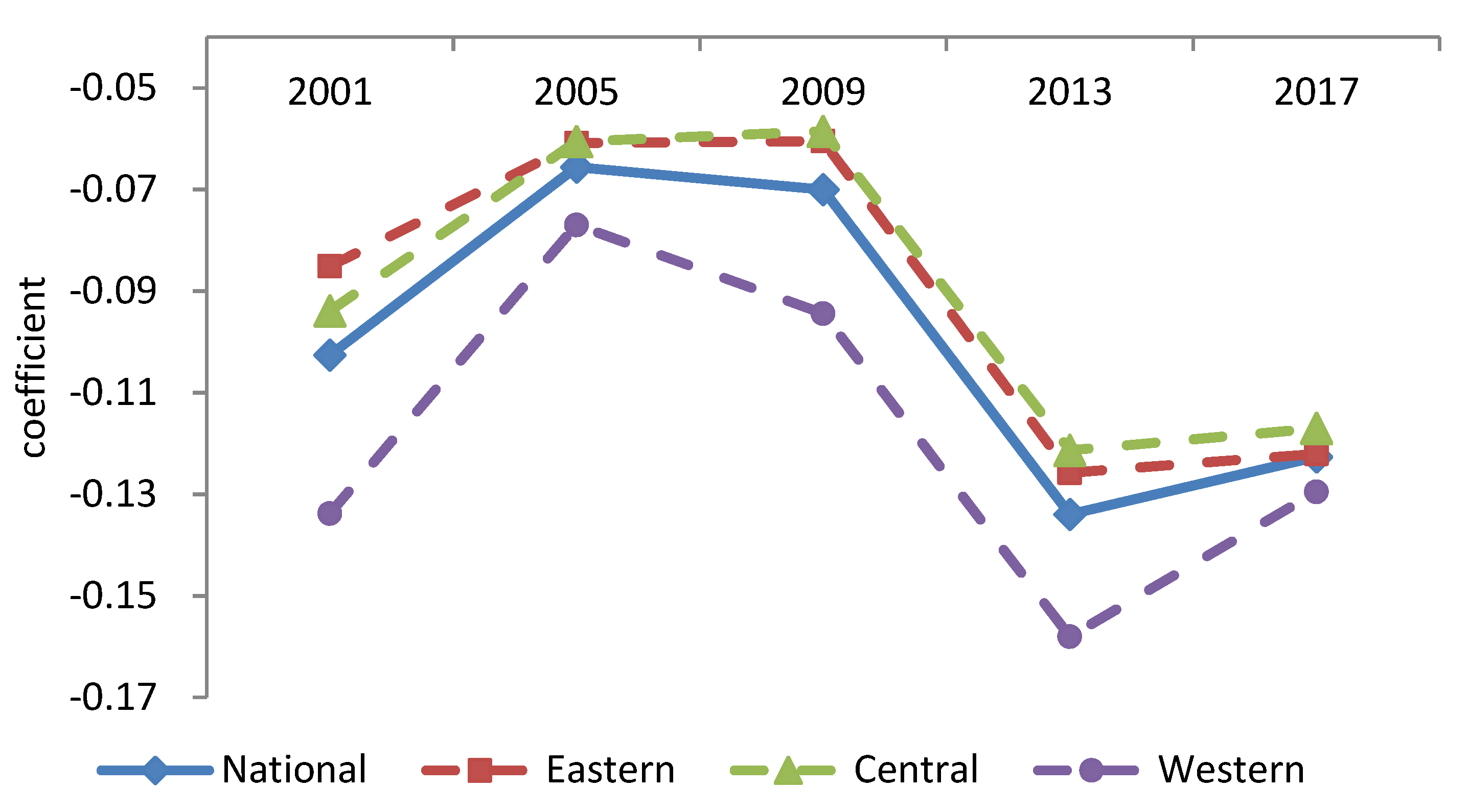
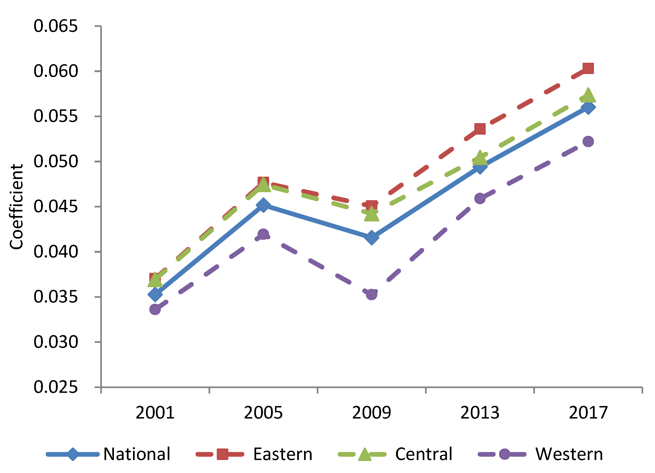
From the regional level, the influence coefficient of hydropower on haze pollution in Western China is the largest, which is much higher than the national average level. However, the influence coefficient of hydropower on economic growth in the eastern region is the largest, which is larger than that in the central and western regions in turn. The development of hydropower resources in the western region can effectively reduce the local haze pollution, but the suppression effect on the haze pollution in the eastern region is relatively small. The influence of hydropower on haze pollution declined first, reached the minimum value around 2005, and then showed an upward trend (Figure 4). Although the western region, which is rich in hydropower resources, is the main producing area of hydropower energy, the effect of hydropower on the economic growth of the western region is less than that of the eastern region, which is poor in hydropower resources. The “West-to-East Power Transmission” project mainly transfers the abundant hydropower in the west and a small amount of hydropower in the central region to the eastern region where power resources are relatively scarce, greatly promoting the rapid economic growth of the eastern region. Moreover, the promoting effect of hydropower on regional economic growth shows a fluctuating upward trend (Figure 5).
From 2000 to 2005, the installed capacity of hydropower generation in China increased by 52.82%, of which the western region grew fastest, reaching 57.78%. During this period, the construction of hydropower station produces more smoke and dust, and has a certain negative impact on the local ecological environment, which leads to the reduction of the inhibitory effect of hydropower on haze pollution. After that, the hydropower station began to operate normally, and the cleaning effect of hydropower generation offset the negative effect of hydropower station construction. From 2005 to 2009, the promotion effect of hydropower on economic growth decreased slightly. The reason may be that China’s GDP increased by 122.71%, while the hydropower generation increased by 55.15%. The hydropower generation failed to meet the energy demands brought by rapid economic growth, leading to increased consumption of fossil energy.
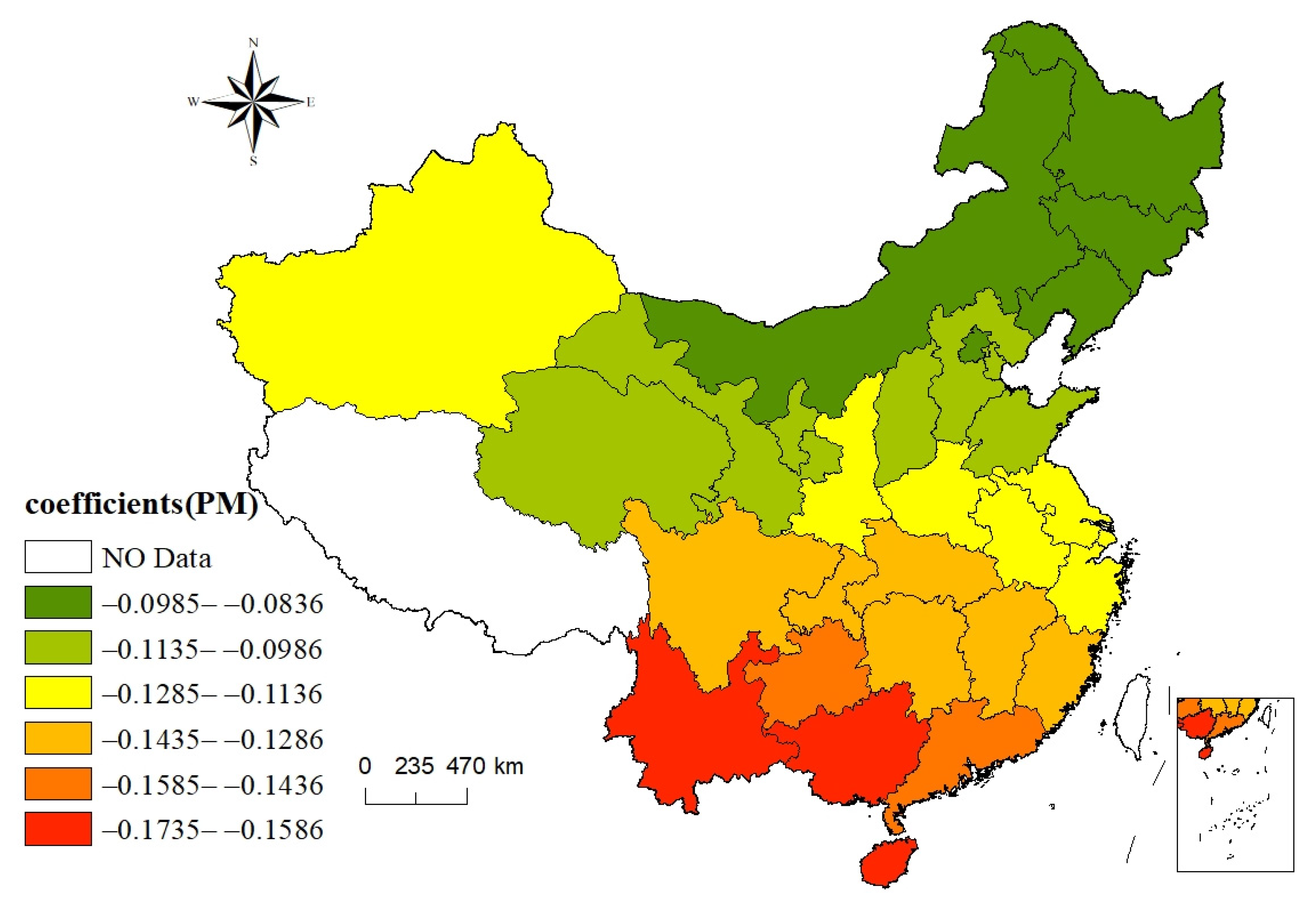
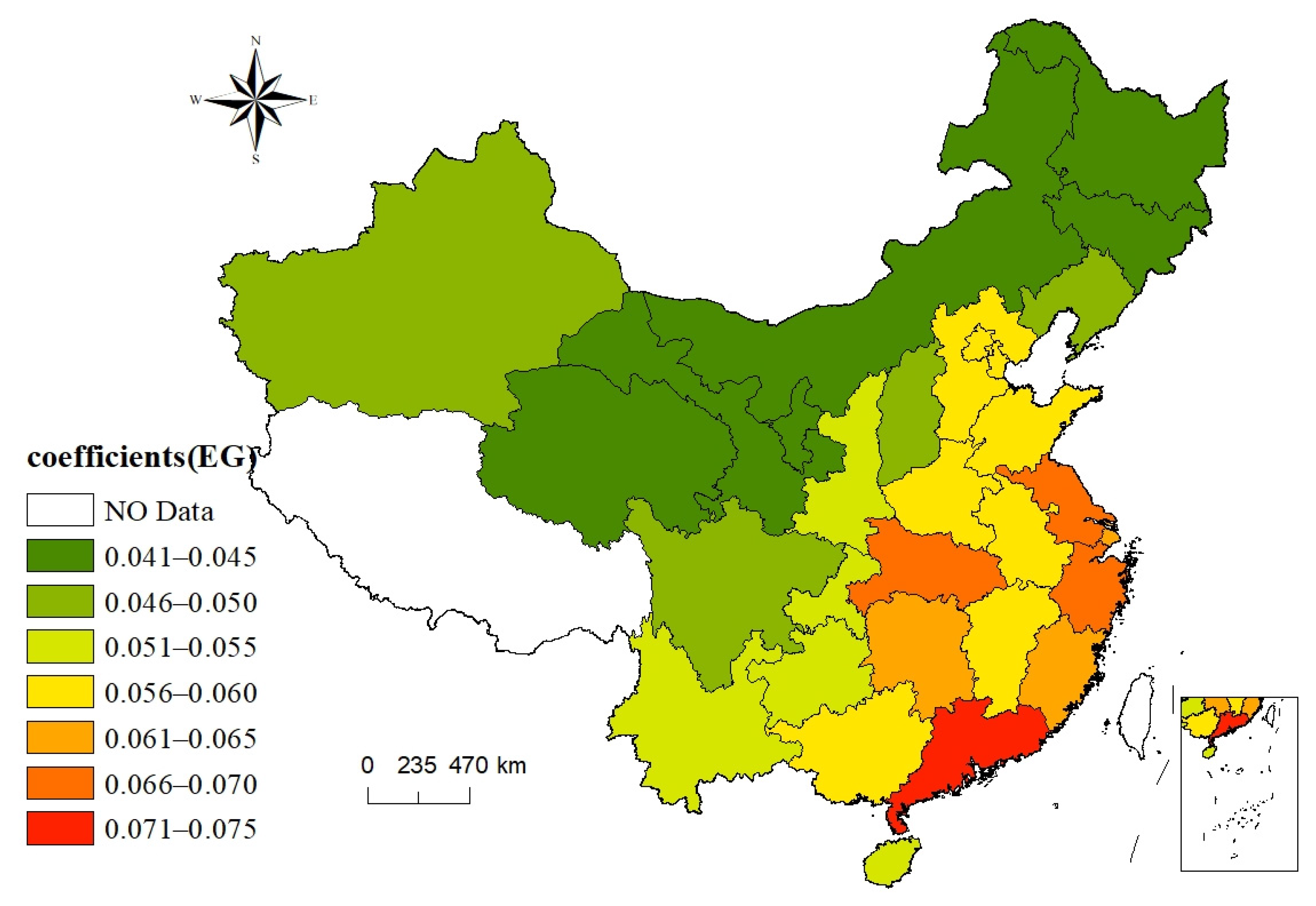
At the provincial level, hydropower has a greater effect on reducing haze reduction in energy production areas than in energy input areas, but hydroelectric power has less of an economic promotion effect on energy production areas than energy input areas. Provinces with better effect of hydroelectric generation on haze emission reduction are mainly concentrated in southwest China, where hydroelectric generation is large, and Guangdong Province, the main input of “West-to-East Power Transmission” of the southern route, including Yunnan (−0.169), Guangxi (−0.168), Hainan (−0.164), Guangdong (−0.154) and Guizhou (−0.152). The provinces with weaker effects of hydropower on haze reduction are mainly concentrated in the three provinces of the northeast and Inner Mongolia (Figure 6). The provinces where hydropower has a greater effect on economic growth are Guangdong (0.0732), Zhejiang (0.0677), Hubei (0.0671), Jiangsu (0.0661) and Shanghai (0.0648). The provinces where hydropower has a lesser effect on economic growth are mainly concentrated in the northeast and northwest regions (Figure 7).

5. Conclusions and Policy Implications

5.1. Conclusions

Based on a Solow growth model, an SDM model was constructed to study the impact of hydropower on regional economic growth. Meanwhile, based on STIRPAT model and EKC hypothesis, an SDM model was built to research the impact of hydropower on haze pollution. The adjacency spatial weight matrix and economic distance space weight matrix are introduced to carry out regression analysis from geographical dimension and social economic dimension, respectively. The GWR model was used to test the spatial heterogeneity of hydropower to regional economic growth and haze pollution. The annual data of hydropower generation, economic growth and haze pollution in 30 provinces in China from 2000 to 2017 were used to study the impact of hydropower on regional economic growth and haze pollution. The main results are as follows.
(1)
Hydropower generation, haze pollution and economic growth in China’s provinces all have significant positive spatial auto-correlation, which is manifested as high-high type and low-low type clustering. Both the positive spatial auto-correlation of haze pollution and economic growth are manifested as spatial “spillover effects” and temporal “superimposed effects”. The difference is that the spatial “spillover effect” of haze pollution is greater than the temporal “superimposition effect”, while the temporal “superimposition effect” of economic growth is greater than the spatial “spillover effect”. When considering both the time and space dimensions, the spatial and temporal lag coefficient of haze pollution is significantly negative, while the spatial and temporal lag coefficient of economic growth is significantly positive;
(2)
Hydropower can significantly promote economic growth. Moreover, the spatial spillover effect of hydropower on economic growth is greater than the local effect, indicating that hydropower has a greater neighboring effect in promoting economic growth in the eastern region through the “West-to-East Power Transmission”. The long-term impact of hydropower on economic growth is greater than the short-term impact;
(3)
Hydropower can significantly inhibit haze pollution. Moreover, the spatial spillover effect of hydropower on haze pollution is greater than the local effect. However, as a transitional stage in the short term, hydropower has not been able to effectively inhibit the haze pollution in the region. In the long term, hydropower can effectively inhibit local and neighboring haze pollution;
(4)
The promotion effect of hydropower on economic growth in the western region is less than that in the eastern region, which further aggravates the economic development gap between the eastern and western regions. The inhibition effect of hydropower on haze pollution in the western region is greater than that in the eastern region.

5.2. Policy Implications

(1)
The regional distribution of China’s hydropower resources is uneven. The western region, especially the southwest region, is rich in hydropower resources and has potential for development. Therefore, the construction of hydropower infrastructure should be strengthened, and the energy structure of the eastern region should be improved with the help of the “West-to-East power transmission” project to reduce haze pollution. In addition, scientific planning for hydropower construction in the western region can effectively transform the resource advantages of the western region into economic advantages and boost the economic development of the western region;
(2)
From a regional perspective, the contribution of hydropower resources to the economic growth of the western region of the main production area is much smaller than that of the eastern region of the importing area, which further exacerbates the economic development gap between the west and the east. The western region should use the “West-to-East Power Transmission” and other large-scale development projects in the western region to transform energy advantages into economic advantages, attract the transfer of eastern and international industries with abundant and cheap clean energy, vigorously develop advantageous characteristic industries, and promote economic development in the western region;
(3)
Regional economic growth has a significant spatial spillover effect, which helps to alleviate regional uneven development. When formulating economic development policies at the national level, we should vigorously guide inter-regional cooperation, especially the cooperation between the east and the west, optimize the cross-regional allocation of resources, and give full play to the spatial spillover effects of economic growth;
(4)
China’s provincial haze pollution has significant spatial spillover effects and temporal superposition effects, which requires haze governance to adopt “joint prevention and control” policy and strengthen long-term regional cooperation. Any unilateral governance activities will be difficult to achieve more significant results due to the spatial spillover effect of haze pollution, and the lax governance in any period will aggravate the haze pollution level in the next period. This requires that haze management adopt a “joint prevention and control” policy and strengthen long-term cooperation among different regions.

Author Contributions

Conceptualization, Z.X., C.L. and T.L.; methodology, C.L. and T.L.; software, T.L.; validation, C.L., and Z.X.; formal analysis, T.L.; investigation, T.L.; resources, C.L., Z.X. and T.L.; data curation, T.L.; writing—original draft preparation, T.L.; writing—review and editing, Z.X. and C.L.; visualization, T.L.; supervision, Z.X. and C.L.; project administration, C.L.; funding acquisition, C.L. All authors have read and agreed to the published version of the manuscript.

Funding

This research was funded by the National Social Science Foundation of China, grant number 17BJY076.

Institutional Review Board Statement

Not applicable.

Informed Consent Statement

Not applicable.

Data Availability Statement

Not applicable.

Acknowledgments

We would like to express our sincere appreciation to anonymous reviewers for valuable suggestions and corrections.

Conflicts of Interest

The authors declare no conflict of interest.

References

  1. Xu, B.; Chen, Y.F.; Shen, X.B. Clean energy development, carbon dioxide emission reduction and regional economic growth. Econ. Res. J. 2019, 54, 188–202. [Google Scholar]
  2. Shao, S.; Zhang, X.; Zhao, X.R. Empirical decomposition and peaking pathway of carbon dioxide emissions of China’s manufacturing sector-generalized divisia index method and dynamic scenario analysis. China Ind. Econ. 2017, 3, 44–63. [Google Scholar]
  3. Chen, S.Y.; Chen, D.K. Air pollution, government regulations and high-quality economic development. Econ. Res. J. 2018, 53, 20–34. [Google Scholar]
  4. Yang, S.Y.; Wang, F.; Liu, N. Assessment of the air pollution prevention and control action plan in China: A difference-in-difference analysis. China Popul. Resour. Environ. 2020, 30, 110–117. [Google Scholar]
  5. Anser, M.K.; Hanif, I.; Vo, X.V.; Alharthi, M. The long-run and short-run influence of environmental pollution, energy consumption, and economic activities on health quality in emerging countries. Environ. Sci. Pollut. Res. 2020, 27, 32518–32532. [Google Scholar] [CrossRef]
  6. Hu, F.X.; He, G.C. Energy-saving and emission reduction benefit analysis on west-to-east transmission project of China southern power grid. Autom. Electr. Power Syst. 2014, 38, 20–24. [Google Scholar]
  7. Yu, Q.Q. Analysis on the competitiveness of trans-provincial and trans-regional hydropower transmission in power market. Water Power 2020, 46, 95–98. [Google Scholar]
  8. Ma, L.M.; Zhang, X. The spatial effect of China’s haze pollution and the impact from economic change and energy structure. China Ind. Econ. 2014, 4, 19–31. [Google Scholar]
  9. Li, L.; Hong, X.; Wang, J. Evaluating the impact of clean energy consumption and factor allocation on China’s air pollution: A spatial econometric approach. Energy 2020, 195, 116842. [Google Scholar] [CrossRef]
  10. Wei, W.X.; Zhao, Y.R. Analysis of feed-in tariff on atmospheric environmental benefits. China Popul. Resour. Environ. 2017, 27, 209–216. [Google Scholar]
  11. Xu, X.L. Impacts of the clean energy subsidy reform on industry development and environment pollution: An analysis based on a dynamic CGE model. J. Shanghai Univ. Financ. Econ. 2018, 20, 44–57. [Google Scholar]
  12. Xie, Y.; Wu, D.; Zhu, S. Can new energy vehicles subsidy curb the urban air pollution? empirical evidence from pilot cities in China. Sci. Total Environ. 2021, 754, 142232. [Google Scholar] [CrossRef]
  13. Dogan, E.; Seker, F. Determinants of CO2 emissions in the European Union: The role of renewable and non-renewable energy. Renew. Energy 2016, 94, 429–439. [Google Scholar] [CrossRef]
  14. Zoundi, Z. CO2 emissions, renewable energy and the Environmental Kuznets Curve, a panel cointegration approach. Renew. Sustain. Energy Rev. 2017, 72, 1067–1075. [Google Scholar] [CrossRef]
  15. Razmjoo, A.; Kaigutha, L.G.; Rad, M.A.V.; Marzband, M.; Davarpanah, A.; Denai, M. A technical analysis investigating energy sustainability utilizing reliable renewable energy sources to reduce emissions in a high potential area. Renew. Energy 2021, 164, 46–57. [Google Scholar] [CrossRef]
  16. Zhang, X.D.; Liu, X.Y. Study on carbon taxation and developing renewable energy—Growth and welfare effects analyses based on OLG-CGE model. China Ind. Econ. 2015, 3, 18–30. [Google Scholar]
  17. Inglesi-Lotz, R. The impact of renewable energy consumption to economic growth: A panel data application. Energy Econ. 2016, 53, 58–63. [Google Scholar] [CrossRef] [Green Version]
  18. Bhattacharya, M.; Paramati, S.R.; Ozturk, I.; Bhattacharya, S. The effect of renewable energy consumption on economic growth: Evidence from top 38 countries. Appl. Energy 2016, 162, 733–741. [Google Scholar] [CrossRef]
  19. Lin, M.S. The clean energy consumption, environment governance and the sustainable economic growth in China. J. Quant. Tech. Econ. 2017, 34, 3–21. [Google Scholar]
  20. Pilatowska, M.; Geise, A. Impact of clean energy on CO2 emissions and economic growth within the phases of renewables diffusion in selected european countries. Energies 2021, 14, 812. [Google Scholar] [CrossRef]
  21. Kahia, M.; Aissa, M.B.; Lanouar, C. Renewable and non-renewable energy use-economic growth nexus: The case of MENA Net oil importing countries. Renew. Sustain. Energy Rev. 2017, 71, 127–140. [Google Scholar] [CrossRef]
  22. Destek, M.A.; Aslan, A. Renewable and non-renewable energy consumption and economic growth in emerging economies: Evidence from bootstrap panel causality. Renew. Energy 2017, 111, 757–763. [Google Scholar] [CrossRef]
  23. Keček, D.; Mikulić, D.; Lovrinčević, Ž. Deployment of renewable energy: Economic effects on the Croatian economy. Energy Policy 2019, 126, 402–410. [Google Scholar] [CrossRef]
  24. Lin, B.Q.; Sun, C.W. How can China achieve its carbon emission reduction target while sustaining economic growth? Soc. Sci. China 2011, 1, 64–76. [Google Scholar]
  25. Dietz, T.; Rosa, E.A. Effects of population and affluence on CO2 emissions. Proc. Natl. Acad. Sci. USA 1997, 94, 175–179. [Google Scholar] [CrossRef] [Green Version]
  26. Cheng, Z.H.; Liu, J.; Li, L.S. Research on the Effects of Industrial Structure Adjustment and Technical Progress on Haze Reduction. China Soft Sci. 2019, 1, 146–154. [Google Scholar]
  27. Gong, M.Q.; Liu, H.Y. The influence of two-way FDI coordinated development and industrial structure evolution on environmental pollution in China. J. Int. Trade 2020, 2, 110–124. [Google Scholar]
  28. Shao, S.; Li, X.; Cao, J.H.; Yang, L.L. China’s economic policy choices for governing smog pollution based on spatial spillover effects. Econ. Res. J. 2016, 51, 73–88. [Google Scholar]
  29. Brunsdon, C.; Fotheringham, A.S.; Charlton, M. Geographically weighted regression: A method for exploring spatial nonstationary. Geogr. Anal. 1996, 28, 281–298. [Google Scholar] [CrossRef]
  30. Xu, B.; Lin, B. Investigating spatial variability of CO2 emissions in heavy industry: Evidence from a geographically weighted regression model. Energy Policy 2020, 149, 112011. [Google Scholar] [CrossRef]
  31. LeSage, J.P.; Pace, R.K. Introduction to Spatial Econometrics; CRC Press: Boca Raton, FL, USA, 2010; pp. 24–53. [Google Scholar]
  32. Zafar, M.W.; Shahbaz, M.; Hou, F.; Sinha, A. From nonrenewable to renewable energy and its impact on economic growth: The role of research & development expenditures in Asia-Pacific Economic Cooperation countries. J. Clean. Prod. 2019, 212, 1166–1178. [Google Scholar]
  33. Saidi, K.; Omri, A. The impact of renewable energy on carbon emissions and economic growth in 15 major renewable energy-consuming countries. Environ. Res. 2020, 186, 109567. [Google Scholar] [CrossRef] [PubMed]
  34. Li, M.; Long, K. Direct or spillover effect: The impact of pure technical and scale efficiencies of water use on water scarcity in china. Int. J. Environ. Res. Public Health 2019, 16, 3401. [Google Scholar] [CrossRef] [Green Version]
  35. van Donkelaar, A.; Martin, R.V.; Brauer, M.; Hsu, N.C.; Kahn, R.A.; Levy, R.C.; Lyapustin, A.; Sayer, A.M.; Winker, D.M. Global estimates of fine particulate matter using a combined geophysical-statistical method with information from satellites. Environ. Sci. Technol. 2016, 50, 3762–3772. [Google Scholar] [CrossRef] [PubMed]
  36. Liu, K.; Lin, B. Research on influencing factors of environmental pollution in China: A spatial econometric analysis. J. Clean. Prod. 2019, 206, 356–364. [Google Scholar] [CrossRef]
  37. Li, K.; Fang, L.; He, L. How population and energy price affect China’s environmental pollution? Energy Policy 2019, 129, 386–396. [Google Scholar] [CrossRef]
  38. Yu, Y.Z.; Zhang, S.H. Urban housing prices, purchase restriction policy and technological innovation. China Ind. Econ. 2017, 6, 98–116. [Google Scholar]
  39. Elhorst, J.P. Matlab software for spatial panels. Int. Reg. Sci. Rev. 2014, 37, 389–405. [Google Scholar] [CrossRef] [Green Version]
  40. Lee, L.; Yu, J. A spatial dynamic panel data model with both time and individual fixed effects. Econom. Theory 2010, 26, 564–597. [Google Scholar] [CrossRef] [Green Version]
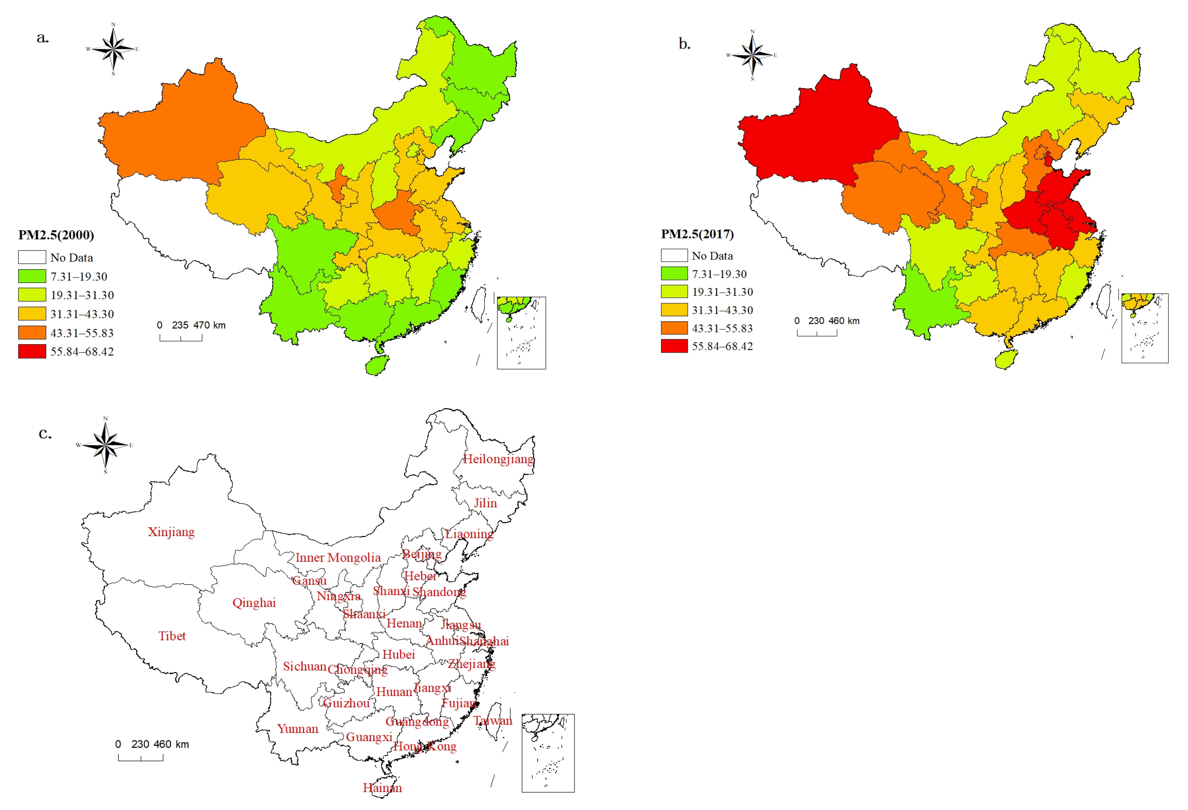
Figure 1. The temporal and spatial distribution of haze pollution (PM2.5 (μg/m3)) in China’s provinces: (a) spatial distribution of haze pollution in 2000; (b) spatial distribution of haze pollution in 2017; (c) a map of China’s provincial administrative districts.
Energies 14 02812 g001
Figure 2. The temporal and spatial distribution of hydropower generation (100 million kWh) in China’s provinces: (a) spatial distribution of hydropower generation in 2000; (b) spatial distribution of hydropower generation in 2017.
Energies 14 02812 g002
Figure 3. The temporal and spatial distribution of economic scale (100 million yuan) in China’s provinces: (a) spatial distribution of economic scale in 2000; (b) spatial distribution of economic scale in 2017.
Energies 14 02812 g003
Figure 4. The impact of hydropower on haze pollution in various regions.
Energies 14 02812 g004
Figure 5. The impact of hydropower on economic growth in various regions.
Energies 14 02812 g005
Figure 6. The impact of hydropower on provincial haze pollution in 2017.
Energies 14 02812 g006
Figure 7. The impact of hydropower on provincial economic growth in 2017.
Energies 14 02812 g007
Table 1. Descriptive statistics of variables.
VariableSymbolDefinitionObservationsMeanS. D.MinMaxSource
Economic growthlnEGReal GDP per capita (ten thousand yuan)5409.7690.7507.88711.718China Statistical Yearbook
Haze pollutionlnPMHaze concentration (μg/m3)5403.5710.4631.9914.437See footnote 1
HydropowerlnHPHydropower generation (100 million kWh)5403.9431.97208.020Almanac of China’s Water Power
Capital stocklnCSPerpetual inventory calculation method (100 million yuan)5409.8310.9607.35911.93China Statistical Yearbook
Labor inputlnEPSum of employed persons (10 thousand people)5407.5510.8205.6198.820China Statistical Yearbook
Technological innovationlnRDInternal expenditure of R&D expenditure (100 million yuan)5404.3721.635−0.1867.759China Statistical Yearbook on Science and Technology
UrbanizationlnURProportion of urban population in total population (%)5403.8550.2983.1444.495China Statistical Yearbook
Population densitylnPDNumber of people per unit area (person/square kilometers)5405.4181.2622.0038.249China Statistical Yearbook
Industrial structureISCalculated according to Petty–Clark theorem5402.2890.1302.0282.801China Statistical Yearbook
Water scarcityWSRatio of water consumption to renewable water resources5400.8491.5100.0319.187China Statistical Yearbook on Environment
Table 2. Results of the applicability test of the spatial panel model.
Test StatisticsModel (4)Model (7)
Chi-Square Valuep ValueChi-Square Valuep Value
LM-lag28.7160.00029.9170.000
R-LM-lag13.1920.00111.9390.001
LM-error547.2620.0001059.8390.000
R-LM-error548.7120.0001049.0140.000
LR test for SLM19.870.00334.060.000
Wald test for SLM21.500.00233.920.000
LR test for SEM16.890.01040.150.000
Wald test for SEM18.190.00638.640.000
Hausman test24.010.00848.010.000
Table 3. 2000–2017 Moran’s I index of China’s provincial hydropower, haze pollution and economic growth.
YearEconomic Dimension Spatial Weight Matrix (W3)Geographical Dimension Spatial Weight Matrix (W1)
Hydropower (HP)Haze Pollution (lnPM)Economic Growth (lnPGDP)Hydropower (HP)Haze Pollution (lnPM)Economic Growth (lnPGDP)
Moran’s IZMoran’s IZMoran’s IZMoran’s IZMoran’s IZMoran’s IZ
20000.100 ***3.9310.089 ***3.5780.091 ***3.6640.380 ***3.4210.452 ***3.9490.457 ***4.065
20010.102 ***4.0080.095 ***3.7350.092 ***3.6810.344 ***3.1620.498 ***4.3040.456 ***4.059
20020.090 ***3.6640.094 ***3.7270.092 ***3.6960.366 ***3.3720.468 ***4.0930.457 ***4.067
20030.086 ***3.5640.112 ***4.2530.093 ***3.7180.307 ***2.9030.470 ***4.1400.460 ***4.085
20040.031 **1.9820.071 ***3.0740.095 ***3.7690.163 **1.8350.420 ***3.7200.464 ***4.107
20050.039 **2.2060.070 ***3.0270.096 ***3.7980.148 **1.6670.423 ***3.7320.466 ***4.114
20060.053 ***2.6200.094 ***3.7310.097 ***3.8190.187 **1.9620.453 ***3.9790.469 ***4.127
20070.055 ***2.6830.082 ***3.3970.096 ***3.8050.219 **2.2570.444 ***3.9020.467 ***4.109
20080.065 ***2.9830.070 ***3.0310.097 ***3.8170.244 ***2.4830.406 ***3.5920.463 ***4.073
20090.063 ***2.9010.065 ***2.9070.096 ***3.8060.264 ***2.6470.365 ***3.2710.459 ***4.029
20100.067 ***3.0260.074 ***3.1490.096 ***3.7990.272 ***2.6600.396 ***3.5250.458 ***4.017
20110.066 ***3.0080.085 ***3.4720.094 ***3.7180.295 ***2.8970.469 ***4.0880.446 ***3.919
20120.076 ***3.2870.071 ***3.0790.092 ***3.6840.338 ***3.2140.394 ***3.5150.438 ***3.847
20130.063 ***2.9330.101 ***3.9210.091 ***3.6410.321 ***3.2280.472 ***4.1040.430 ***3.782
20140.062 ***2.9080.081 ***3.3530.089 ***3.5930.338 ***3.4150.388 ***3.4710.423 ***3.719
20150.066 ***3.0580.103 ***4.0020.088 ***3.5530.360 ***3.6430.434 ***3.8290.418 ***3.682
20160.061 ***2.9090.111 ***4.2140.087 ***3.5290.316 ***3.2630.474 ***4.1370.419 ***3.688
20170.051 ***2.6090.093 ***3.7010.087 ***3.5410.314 ***3.2880.451 ***3.9440.421 ***3.706
Note: **, *** mean significant at the levels of 5%, and 1%, respectively.
Table 4. Empirical results of the impact of hydropower on regional economic growth.
VariableEconomic Dimension Spatial Weight Matrix (W3)Geographical Dimension Spatial Weight Matrix (W1)
(1) SDM(2) SDM(3) DSDM(4) SDM(5) SDM(6) DSDM
W*lnEG0.2535 ***
(4.757)
0.2441 ***
(4.677)
0.8016 ***
(5.007)
0.3148 ***
(5.227)
0.3116 ***
(5.108)
0.3964 **
(2.460)
lnEGt−1 1.0035 ***
(82.151)
0.9666 ***
(74.948)
W*lnEGt−1 0.5248 ***
(2.755)
0.1395 **
(2.235)
lnHP 0.0323 ***
(4.171)
0.0075 ***
(3.330)
0.0369 ***
(4.691)
0.0094 ***
(4.031)
lnCS0.3416 ***
(16.343)
0.3564 ***
(16.924)
0.0137 **
(2.255)
0.3739 ***
(17.541)
0.3905 ***
(18.284)
0.0179 **
(2.438)
lnEP−0.0015
(−0.459)
0.0012
(0.355)
0.0002
(0.174)
0.0063 **
(2.171)
−0.0034
(−1.159)
−0.0001
(−0.128)
lnRD0.0448 ***
(3.198)
0.0348 **
(2.496)
0.0028
(0.683)
0.0429 ***
(3.084)
0.0334 **
(2.393)
−0.0057
(−1.376)
lnUR0.2800 ***
(6.762)
0.2267 ***
(5.186)
−0.0088
(−0.637)
0.2356 ***
(5.428)
0.1952 ***
(4.414)
0.0254 *
(1.797)
WS−0.0077 *
(−1.896)
−0.0041 *
(−1.844)
−0.0036 **
(−2.330)
−0.0020 **
(−2.412)
−0.0019 **
(−2.387)
−0.0040 **
(−2.535)
W*lnHP 0.0391 *
(1.857)
0.0303 **
(2.324)
0.0113 *
(1.862)
0.0151 ***
(3.549)
W*lnCS−0.5598 ***
(−3.869)
−0.5979 ***
(−3.960)
−0.3247 ***
(−6.239)
−0.1586 ***
(−4.023)
−0.1565 ***
(−3.852)
−0.0510 ***
(−3.109)
W*lnEP0.0539 **
(2.268)
0.0480 **
(2.052)
0.0223 ***
(3.368)
0.0024
(0.372)
0.0038
(0.592)
0.0019
(1.009)
W*lnRD−0.1835 **
(−2.165)
−0.1366
(−1.623)
−0.1032 ***
(−3.897)
0.0378
(1.502)
0.0524 **
(2.088)
0.0071
(0.934)
W*lnUR0.5323 *
(1.832)
0.4049
(1.329)
−0.0179
(−0.182)
−0.0657
(−0.866)
−0.1539 **
(−1.967)
−0.0294
(−1.138)
W*WS−0.0031
(0.103)
−0.0040
(−0.135)
0.0185
(1.055)
−0.0259 **
(−2.444)
−0.0191
(−1.282)
−0.0095 ***
(−2.731)
R20.81980.82340.98560.98050.98060.9985
Log-Likelihood851.3698860.7785−2.303 × 10⁵−2.303 × 10⁵−2.303 × 10⁵−835.4572
Observations540540510540540510
Note: *, **, *** mean significant at the levels of 10%, 5%, and 1%, respectively. The values in parentheses are t statistics.
Table 5. Decomposition results of the impact of hydropower on regional economic growth.
VariableShort-Term ImpactLong-Term Impact
Direct EffectIndirect EffectTotal EffectDirect EffectIndirect EffectTotal Effect
Economic dimension spatial weight matrix (W3)
lnHP0.0147 ***
(2.717)
0.0273 ***
(2.807)
0.0420 ***
(3.004)
0.1123 ***
(2.811)
0.1824 ***
(2.809)
0.2947 ***
(2.919)
Geographical dimension spatial weight matrix (W1)
lnHP0.0100 ***
(4.504)
0.0178 ***
(4.046)
0.0278 ***
(5.766)
0.0217 **
(2.316)
0.0471 ***
(3.734)
0.0688 **
(2.370)
Note: **, *** mean significant at the levels of 5%, and 1%, respectively. The values in parentheses are t statistics.
Table 6. Empirical results of the impact of hydropower on haze pollution.
VariableEconomic Dimension Spatial Weight Matrix (W3)Geographical Dimension Spatial Weight Matrix (W1)
(1) SDM(2) SDM(3) DSDM(4) SDM(5) SDM(6) DSDM
W*lnPM0.5045 ***
(4.857)
0.5055 ***
(4.878)
0.6389 ***
(7.992)
0.6845 ***
(18.305)
0.6806 ***
(18.064)
0.6740 ***
(17.221)
lnPMt−1 0.4045 ***
(9.903)
0.3105 ***
(7.179)
W*lnPMt−1 −0.6500 **
(−2.359)
−0.1715 **
(−2.446)
lnHP −0.0100 *
(−1.661)
−0.0044 *
(−1.711)
−0.0057 **
(−2.314)
−0.0047 *
(−1.801)
lnEG−1.1150 ***
(−3.694)
−0.9763 ***
(−3.195)
−0.3498
(−1.289)
−0.0881
(−0.352)
−0.0379
(−0.150)
−0.0600
(−0.248)
(lnEG)20.0513 ***
(3.572)
0.0434 ***
(2.970)
0.0131
(1.003)
0.0040
(0.337)
0.0008
(0.064)
0.0021
(0.181)
lnPD−0.5272 ***
(−3.452)
−0.5136 ***
(−3.337)
−0.3765 ***
(−2.809)
−0.1233
(−0.887)
−0.1242
(−0.889)
−0.2241 *
(−1.674)
lnRD−0.0713 **
(−2.543)
−0.0627 **
(−2.197)
−0.0287 **
(−2.170)
−0.0701 ***
(−3.278)
−0.0704 ***
(−3.261)
−0.0432 **
(−2.179)
IS0.0339
(0.201)
0.0576
(0.339)
0.0077
(0.052)
−0.2530 **
(−2.019)
−0.2578 **
(−2.055)
−0.0755
(−0.646)
WS−0.0010
(−0.103)
0.0006
(0.062)
−0.0090
(−0.964)
0.0076
(0.949)
0.0079
(0.990)
0.0009
(0.115)
W*lnHP −0.2146 **
(−2.425)
−0.1542 **
(−2.053)
−0.0410 *
(−1.797)
−0.0439 **
(−2.091)
W*lnEG−6.3202 ***
(−3.962)
−6.5048 ***
(−4.007)
−3.7250 **
(−2.557)
−2.2495 ***
(−5.553)
−2.2356 ***
(−5.427)
−0.9907 **
(−2.486)
W*(lnEG)20.2775 ***
(3.716)
0.2729 ***
(3.576)
0.1494 **
(2.145)
0.1025 ***
(5.148)
0.0992 ***
(4.810)
0.0401 **
(2.008)
W*lnPD−0.9865
(−0.869)
−1.7886
(−1.522)
−0.4225
(−0.414)
−1.0321 ***
(−4.138)
−1.1132 ***
(−4.387)
−0.5429 **
(−2.253)
W*lnRD−0.4353 **
(−2.452)
−0.2799
(−1.490)
−0.4485 ***
(−2.576)
−0.0255
(−0.584)
−0.0030
(−0.066)
−0.0281
(−0.671)
W*IS−1.7738
(−1.125)
−1.0813
(−0.679)
−2.7553 **
(−1.976)
0.1697
(0.604)
0.1674
(0.597)
−0.1962
(−0.747)
W*WS0.1241 **
(2.000)
0.1328 **
(2.145)
0.0979 *
(1.748)
−0.0136
(−0.770)
−0.0127
(−0.719)
−0.0150
(−0.834)
R20.22850.22710.12890.22150.21770.0968
Log-Likelihood−2.303 × 10⁵−2.303 × 10⁵−5.222 × 10⁴−5.222 × 10⁴−5.222 × 10⁴−2784.1154
Observations540540510540540510
Note: *, **, *** mean significant at the levels of 10%, 5%, and 1%, respectively. The values in parentheses are t statistics.
Table 7. Decomposition results of the impact of hydropower on haze pollution.
VariableShort-Term ImpactLong-Term Impact
Direct EffectIndirect EffectTotal EffectDirect EffectIndirect EffectTotal Effect
Economic dimension spatial weight matrix (W3)
lnHP−0.0150
(−0.954)
−0.4489 *
(−1.670)
−0.4639 *
(−1.663)
−0.0053 **
(−2.255)
−0.2553 *
(−1.933)
−0.2606 *
(−1.926)
Geographical dimension spatial weight matrix (W1)
lnHP−0.0062
(−0.474)
−0.1152 *
(−1.845)
−0.1214 *
(−1.708)
−0.0124 **
(−2.294)
−0.2085 *
(−1.654)
−0.2209 **
(−2.366)
Note: *, ** mean significant at the levels of 10% and 5%, respectively. The values in parentheses are t statistics.
Table 8. Robustness test results of the impact of hydropower on regional economic growth.
VariableEconomic Dimension Spatial Weight Matrix (W3)Geographical Dimension Spatial Weight Matrix (W1)
(1) SDM(2) DSDM(3) SDM(4) DSDM
W*lnEG0.3000 ***
(2.883)
0.1998 ***
(2.911)
0.3911 ***
(6.803)
0.3042 ***
(5.383)
lnEGt−1 0.9718 ***
(77.158)
1.0850 ***
(79.572)
W*lnEGt−1 1.2800 ***
(6.365)
0.1055 ***
(2.948)
lnHIC0.0383 ***
(4.757)
0.0064 ***
(2.711)
0.0411 ***
(5.782)
0.0060 ***
(2.626)
W*lnHIC0.0492 **
(2.217)
0.0833 ***
(6.186)
0.0716 *
(1.801)
0.0253 ***
(4.856)
Control variableYESYESYESYES
R20.70990.99500.97890.9984
Log-Likelihood−2784.1154−2.030 × 10⁵−2.030 × 10⁵−7057.0562
Note: *, **, *** mean significant at the levels of 10%, 5%, and 1%, respectively. The values in parentheses are t statistics.
Table 9. Robustness test results of the impact of hydropower on haze pollution.
VariableEconomic Dimension Spatial Weight Matrix (W3)Geographical Dimension Spatial Weight Matrix (W1)
(1) SDM(2) DSDM(3) SDM(4) DSDM
W*lnPM0.5100 ***
(4.954)
0.6376 ***
(7.971)
0.6829 ***
(18.263)
0.6805 ***
(17.608)
lnPMt−1 0.4026 ***
(9.800)
0.3079 ***
(7.099)
W*lnPMt−1 −0.6798 **
(−2.485)
−0.1667 **
(−2.382)
lnHIC−0.0140 ***
(−3.115)
−0.0074 **
(−2.240)
−0.0066 **
(−2.217)
−0.0105 *
(−1.713)
W*lnHIC−0.1017 **
(−2.231)
−0.1547 **
(−2.100)
−0.0401 **
(−2.209)
−0.0509 *
(−1.895)
Control variableYESYESYESYES
R20.23070.12560.22590.0950
Log-Likelihood−7057.0562−6.668 × 10⁴−6.668 × 10⁴−1635.2995
Note: *, **, *** mean significant at the levels of 10%, 5%, and 1%, respectively. The values in parentheses are t statistics.
Publisher’s Note: MDPI stays neutral with regard to jurisdictional claims in published maps and institutional affiliations.