Extended Exergy Analysis (EEA) of Italy, 2013–2017

Abstract

In recent years, many studies have been published on the applications of exergy analyses to complex systems, including entire countries. Oddly, the results, although consistent, appear to lead to divergent conclusions. The underlying problem is that in a “pure” thermodynamic analysis, the so-called “externalities”, i.e., labor, capital, and environmental costs, are often neglected or only approximately included in the picture. In 1998, an extension of the theory that included the exergy content of the externalities was introduced, called “extended exergy accounting” (EEA). Its novelty consisted of the explicit inclusion of the exergy embodied in the externalities. The aim of this work is to use the results of the extended exergy accounting to obtain an indicator that can be used to assess the sustainable development of a country. First, a novel methodological approach to the theory is presented, based on the exploitation of a very large dataset obtained from several national and European statistical institutions. After a brief discussion of the theory, an application to the case of Italy is developed over a 5 years time window (2013–2017). The paper includes a comparison with the concurrent evolution of other sustainability indicators and of the gross domestic product (GDP) indicator. The results show a consistent trend for EE as compared with those of other indicators, and also convincingly proves that this trend is incompatible with that of the GDP. The EE indicator is called the exergy footprint, which also displays a remarkable sensitivity to both environmental and economic factors.

1. Introduction

According to a recent United Nations report [1], the human population is expected to reach 8.5 billion by 2030, 9.7 by 2050, and 10.9 by 2100. Considering the obvious need to grant decent life standards to as many people as possible, the discussion about “sustainable growth” is becoming a priority item for politicians, economists, and the public at large. In 2015, 193 countries endorsed the 2030 Agenda for Sustainable Development, setting several “sustainable goals” to be accomplished no later than 2030 [2]. Within this framework, it is quite clear that it is necessary for analysts to produce an environment indicator (or a set of indicators) suggestive of the actual evolution and state of the environment, which can show whether a country or region is moving in the right direction. On the other hand, the available data sets are too often pre-filtered by barely objective (and at times completely unscientific) considerations, especially because of the enormous political and economic interests involved. In fact, for more than seventy years, gross domestic product (GDP) has been the main tool adopted by economic agencies, political organizations, state institutions, and the media to assess the “health” of a community. Many scientific papers convincingly point to the unsuitability of this choice, since GDP was conceived to evaluate only the “marketable” part of a society to manage war efforts during WW2 [3,4,5]. Referring in particular to the issue of the management of natural resources, the information that one can extract from GDP may lead to misleading conclusions. Let us consider for example the case of deforestation: given that the harvesting of live trees and marketing of their wood are attributed an economic value, their contribution to the GDP will be positive, although this might be a disaster from a sustainability point of view. Against this background, several indicators were developed in the last years, aiming to replace or supplement the GDP [5]: the Index of Sustainable Economic Welfare [6], the Ecological Footprint [7], the Subjective Well-Being [8], the Human Development Index [9], and the Living Planet Report [10] indicators. In spite of these intellectual efforts, the problem is far from being solved: each one of the above indices focuses only on some aspects of the problem, or worse is based on totally subjective issues such as the “happiness of a population”. This may also be the reason why GDP is currently still the main decision-making tool for most countries.

The rationale of the present work is to use the very large amount of data available from several national and private institutions to derive a sustainability index based on the exergy consumption of the streams of materials, energy, labor, and capital involved in the balance of a community (in the case discussed here, of a whole country), considered as a thermodynamic system, and thus “enclosed” within the boundaries set by the analyst. Why consider exergy instead of energy? Currently, national energy balances are available for most countries (e.g., [11,12,13]) and present an accurate and sufficiently disaggregated balance of all of the material and energy streams throughout a country; however, since these national energy budgets make use only with of the first law of thermodynamics and neglect the “quality” of the streams involved, it is difficult to derive useful second law insights.

The term exergy is ascribed to the Slovenian Zoran Rant [14] and quite literally means “externally available technical work”, i.e., the net amount of energy that can be used for real technical purposes, neglecting the amount degraded (and becoming unavailable) in the inevitably non-reversible processes that compose any conversion chain and are evidenced by an increase in entropy. The method of exergy analysis was developed in the 1970s by Gaggioli, Moran, Fratzscher, Bayer, Szargut, and many others [15]. Plenty of published studies have testified to the application of the method of exergy analysis (herein referred to as “EA”) as a basis for studies performed on industrial systems and countries, e.g., [16,17,18,19,20,21,22]. The exergy method undoubtedly represents a welcome improvement towards the assessment of the exploitation of the primary resources that feed the final energy use, although too many factors are still left out of the picture when one considers the exergy balances of a whole community, a country, or in general a complex system. With specific reference to the modeling of the complex flows of information that characterize a modern society, perhaps the main limitation is the neglection of the circulation of financial resources or of the socioeconomic circumstances under which a society operates. The key issues here are the so-called “externalities” (labor, capital, environmental costs); these are not explicitly considered in the context of a simple EA, which represents at once its strength (rigorous rooting in thermodynamics) and its weakness (social systems do not evolve using thermodynamics alone). In light of these considerations, the algorithm of the EA was extended by “internalizing externalities”, which can be done adopting either a second-law-based monetary accounting approach (thermo-economics—TE) or the purely resource-based extended exergy analysis (EEA) approach. The latter method consists of associating the energy carriers for all streams contributing to the supply-and-production chain to labor, capital, and remediation costs and their embodied primary exergy, thus eliminating from the picture a direct recourse to monetary considerations. As a matter of fact, the main difference between TE and EEA is that the former leads to a monetary cost (which is much appreciated by industrial analysts), while the latter to a “capital-less” primary exergy cost. EEA has been successfully applied to different societies [23,24,25,26,27] and has been proven to be a realistic, rigorous, and consistent resource consumption indicator.

The aim of this work is to investigate the feasibility of using the EEA as a sustainability indicator. This study consists of the following steps:

(1)

The introduction of a novel procedure for EEA based on the exploitation of the very disaggregated datasets currently available from national and private institutions in order to improve the accuracy of the model;

(2)

The analysis of Italian society over a 5 yea (2013–2017) window of observation in order to extract new useful insights and to critically assess the trends of exergy destruction and of the extended exergy of Italy vs. that of the GDP within the same time-window;

(3)

A comparison of the trends of the EE of Italy and of other sustainability indicators (HDI, ecological footprint, and biocapacity);

(4)

A discussion of the results and conclusions.

1.1. Exergy-Based Analysis: Thermoeconomics, Cumulative Exergy Content, Extended Exergy Analysis

The first exergy-based method proposed in the literature for the analysis of industrial plants was Thermoeconomics (Exergo-Ökonomie in Germany) [28,29]. Rant 1956 [14] is actually credited with the original proposal of the name (ex-ergy, as in “external useful work”). The aim of TE is to find a compromise between a purely thermodynamic analysis, involving exergy, and a purely economic analysis, involving monetary costs; in TE, the monetary cost of a commodity or a production process is allocated to the exergy content of each stream involved. The method, thus, takes into account capital and labor costs and then converts each exergy flow into its monetary cost. The cost per unit of exergy of a product is obtained by summing the capital (CAPEX) and operation (OPEX) costs of all of the involved components. Even from this simplified description it should be clear that it is difficult to apply TE to the analysis of a country or a system that includes “non-marketable” commodities; for instance, TE cannot satisfactorily deal with what has come to be known as “natural capital”.

A method independent from a monetary approach was developed by Jan Szargut in 1967 [30] and later refined by Szargut himself and Antonio Valero and coworkers [31,32]. The “cost” of a physical asset is expressed only in terms of its exergy content, considering the whole supply chain, from start to finish. The added value within the supply chain is taken into account by adding the exergy cost of the process to the exergy of the raw materials (called CExC, cumulative exergy content).

The EEA method was first presented by Gliwice [33] and further developed in subsequent studies [34,35]; the underlying rationale is to assign equivalent exergy values to the externalities according to the following fundamental assumptions:

• By denoting ${\dot{E}}_{in}$ [W] as the total exergy influx into the system country, it must be considered that a portion of it is necessarily spent to ensure the survival and growth of the population, this portion is called “exergy of labor” ${\dot{EE}}_L$ and is computed as α ${\dot{E}}_{in}$ where α < 1 is an econometric coefficient not specified by the theory, which must be derived from the exergy budget of the country under study [35];
• The monetary circulation M2 is converted into the so-called extended exergy of capital by means of another econometric factor β: ${\dot{EE}}_K=\beta {\dot{EE}}_L=\alpha \beta {\dot{E}}_{in}$. This second econometric parameter β is also external to the theory and must be extracted from monetary circulation data for the country;
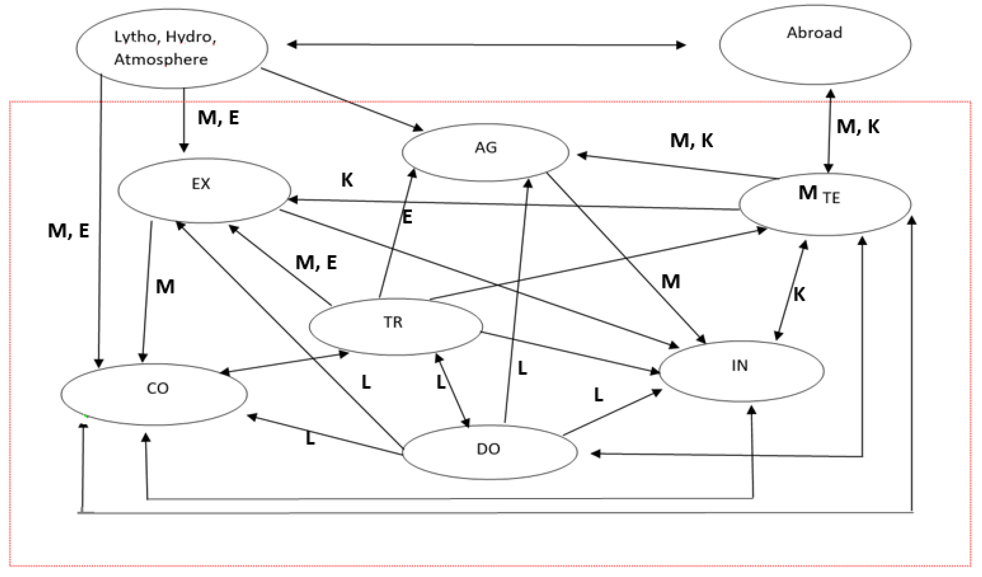
• The system country is subdivided in 7 sectors:
  • Domestic (DO): Power-consuming activities for survival and growth of the human population;
  • Extractive (EX): Involves the processes of mining and quarrying;
  • Conversion (CO): Includes energy conversion, heat and power plants, oil refineries, other refineries and base chemistry industries;
  • Industrial (IN): Includes all of the manufacturing activities that generate added value to raw materials;
  • Transportation (TR): Covers transportation services, both commercial and private;
  • Tertiary (TE): Includes commercial, financial, and service sectors (government, schools, police, etc.);
  • Agricultural (AG): Includes harvesting, forestry, fishing.
• The system exchanges flows of matter and energy with two additional sectors: the environment, from which raw materials are mined, and the other countries or societies collectively grouped into a generic sector called “abroad”.

The extended exergy of a generic commodity “C” is computed as:

$$EEc=CEx{C}_m+CEx{C}_e+E{E}_l+E{E}_k+E{E}_{env}$$

(1)

where EE_c is the extended exergy of the commodity, CExC_m is the cumulative exergy content of materials involved, CExC_e is the cumulative exergy content of the energy involved, EE_l is the extended exergy of labor, EE_k is the extended exergy of capital, and EE_env is the extended exergy associated with the environmental remediation. All of the terms of Equation (1) are homogeneously measured in joules (per unit of product, since EE is a cost function). Different types of exergy streams are exchanged among the different sectors, with each sector “destroying” part of its exergy inflow. The aim of an exergy analysis is in fact the calculation of the rate of exergy destruction and the identification of its causes, so as to gather information useful for the optimization of a single sector or of the whole system. The extended exergy represents instead the amount of primary exergy “embodied” in a material or immaterial commodity and is expressed in J/unit. When considering a complex system such as in this study, a cumulative extended exergy “of the country” can be calculated as the sum of all of the EE values of the goods and services “flowing” through the system.

1.2. The Human Development Index (HDI)

The Human Development Index (HDI) was introduced by the United Nations Development Program (UNDP) in 1990 in their Report HDR-1990 [9]. The rationale behind the HDI is to provide an alternative gauge of the wellness of a country based on a set of socioeconomic parameters: ageing potential, literacy, and pro capite income [36]. The HDI is normalized between 0 and 1: the closer to 1, the higher the standard of living in that specific country. It is the result of the aggregation of three indices [36].

• Long and healthy life. This index is based on life expectancy, defined as “the number of years a newborn could expect to live if prevailing patterns of age-specific mortality rates at the time of birth were to stay the same throughout the child’s life”, considering 20 years and 85 years as limit values. The data are taken from the yearly UN World Population Prospects reports. Once the data for a specific country are available, the dimensional index is computed as:

  $$I_{health}=\frac{actual value-minimum value}{maximum value-minimum value}$$

  (2)
• Knowledge. This index consists of two parameters: (1) average number of years spent on educational activities by adults over 25; (2) expected years of schooling for children of school age. The indicators are normalized by considering a minimum value of 0 and a maximum value of 15 for average school years and 18 for expected years of schooling. The knowledge index is computed from these two parameters by computing for each of them a dimensionless value according to Equation (2) and eventually an arithmetic average in order to obtain the value for the index related to knowledge, I_education. Data are taken from the UNESCO database and from statistical agencies.
• Decent standard of living. This index is based on income; it is measured by the logarithm of the pro capite GNI (gross national income) adjusted by the purchasing power parity (PPP). The minimum PPP value is considered 100$ and the maximum is 75,000$. The index is computed as:

  $$I_{income}=\frac{\ln \left[actual income\right]-\ln \left[minimum income\right]}{\ln \left[actual income\right]-\ln \left[minimum income\right]}$$

  (3)

In Equation (3), the logarithm takes into account the relative spread in the personal income groups within a country. Data are taken from the World Bank and the International Monetary Fund.

The overall HDI is computed by taking the geometric mean of the three-dimensional indices I_k:

$$HDI=\sqrt[3]{I_{Health}+I_{Education}+I_{Income}}$$

(4)

The HDI is widely used in social, economic, and also energy-related fields, which does not imply that the index is free from criticism [36]; over the past 20 years it has received several negative evaluations from the scientific community related to its conception, its methodology, the quality of collected data, the underlying assumptions, and most importantly the fact that it does not contain any reference to the state of the environment.

1.3. Ecological Footprint and Biocapacity

The concept of EF accounting was developed in the 1990s [7]. It is an ecological indicator whose aim is to assess whether a society is consuming renewable resources and disposing of waste at a “sustainable” pace. “Non-renewable” sources are taken into account only for their impact on bioproductive capacity. The EF is defined as the bioproductive area (land and sea) that would be required to maintain sustainable consumption of renewable resources and is computed [37,38] as consumption (kg) multiplied by production efficiency (hectares/kg) according to:

$$E{F}_{Production}=\frac{P}{Y_w}·EQF$$

(5)

where P is the production (or harvest) in tons per year, $Y_w$ is the world average yield in tons per hectare per year, and EQS is an equivalence factor [38].

In essence, the EQF is the ratio of a given land type’s average global productivity divided by the average global productivity of the entire planet’s productive surfaces. The EF of production is computed for each product (e.g., wheat, crops, rice, etc.) using Equation (5) and then the individual contributions are summed up for a specific country. The method also takes into account imports and exports—the algebraic sum of the total EF of import and exports is added to the EF of products to obtain the total EF [7]:

$${EF}_{Consumption}={EF}_{Production}+{EF}_I-{EF}_E$$

(6)

where ${EF}_{Consumption}$ is the net ecological footprint of the country and $E{F}_I-E{F}_E$ is the net amount of EF from imports.

The trend of EF is often associated with that = of another indicator, the biocapacity (BC). BC measures the productivity of the various ecosystems of a region (e.g., arable land, pasture, forest, etc.) [7] and can be measured similarly to EF in hectares:

$$BC=A_n·\frac{Y_n}{Y_w}·EQF$$

(7)

where A_n is the area of country n for a specific product in hectares; $\frac{Y_n}{Y_w}$ is the ratio between the national average yield for a specific product and the world average yield, both measured in tons per hectare per year; and EQF is the same equivalence factor as in Equation (5). All of the considered products are then summed up to obtain the BC parameter of the country.

The algebraic difference between EF and BC is called the “ecological deficit” if it is negative and the “ecological reserve” if positive. In fact, the model includes an exchange (by trade) between countries in “ecological deficit” and countries with an “ecological reserve”, performed via the EF of imports and exports. In spite of its attractiveness and of the simple and very intuitive way in which the results can be represented, the EF method has its own drawbacks, since it includes only the renewable parts of the energy flows, so that the fossil fuel contribution is not taken into account (the BC is also necessary to capture CO₂), which strongly limits its range of application; for example, the disposal of materials with long biodegradation times, such as heavy metals, radioactive waste, and industrial sludge, is beyond the boundaries of the BC model. Additional concerns have been voiced by the scientific community about the rather obscure rationale behind the computation of the equivalence factors, the reliability of the data sources, and the choice of parameters [7,38].

2. Materials and Methods

Here, a method is proposed for collecting data within the context of an EEA. The very extensive and detailed amounts of data made available by governmental authorities, statistical agencies, utility companies, and industries make it possible to implement a structured “data bank”, from which it is possible to derive more realistic results with hitherto unprecedented accuracy. Before proceeding, it is necessary to dispel an objection raised in the late 1980′s by exergy critics, namely that since the system is in a continuous state of non-equilibrium, “instantaneous” balances make little sense, and thus the results are devoid of rigor. This remark is of course correct from a classical thermo viewpoint, in which time is not a relevant parameter, but is surely biased when referring to the macro-scale analysis discussed here for the follow reasons:

• Every thermodynamic analysis of real processes is made under the (explicit or implicit) assumption of quasi-equilibrium transformations. In fact, only rather elementary processes can be approached using a non-equilibrium thermo process, and even then only under somewhat stringent additional assumptions. Thus, exergy analyses of current industrial processes are generally presented in the literature “as design points” and “from a quasi-equilibrium perspective” (often, this second statement is even omitted);
• To consider the evolution in time of a country (or of any other large complex system), a series of arbitrarily frequent energy balances must be considered. In the limit, if Δt- > 0, it is customary to say that we are performing a “transient simulation”. A better description would be “we have a series of infinitely close snapshots of a slightly more complex phenomenon”. This “snapshot” idea and practice is omnipresent; steam and gas turbines, heat exchangers, combustors, and chemical reactors are simulated “in steady state”, meaning that all of the snapshots show the system’s state as being “unvarying” in each considered Δt;
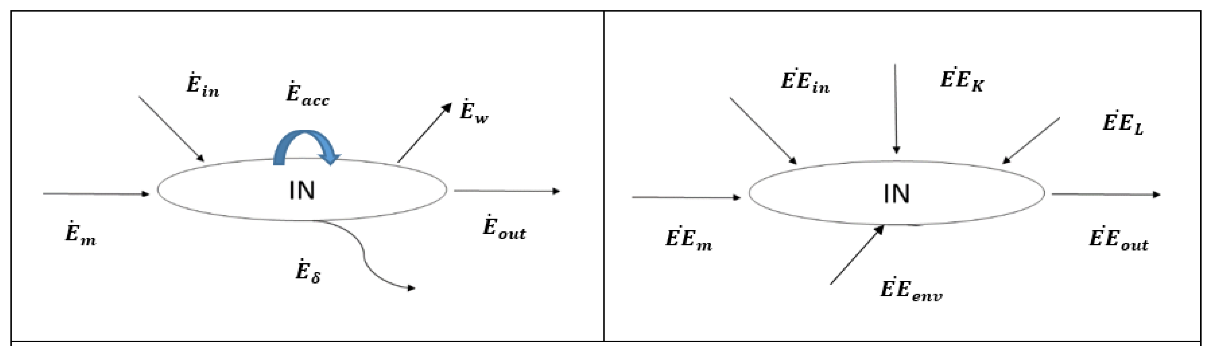
• In processes where the stationary state is not considered a good approximation (internal combustion engines for example, but also more fundamental phenomena such as turbulence), the snapshots are taken at time intervals that are sufficiently close to represent a “continuum” and sufficiently far apart to make changes discernible. From this time-averaged perspective, energy is conserved in each Δt interval. Changes in size or mass of the system are accounted for by including a proper accumulation term;
• Turning now to our “system country”, at each Δt not all of the ${\dot{E}}_{in} - {\dot{E}}_{out}$ difference is destroyed—a portion goes into E_accumulated. However, when we talk about EE (extended exergy), the situation is quite different. EE is essentially a cost, and as with any cost balance, be it instantaneous, discrete, or with or without accumulation, it must as close to zero as allowed by the data disaggregation and accuracy. If we recall that the specific extended exergy ee measures the amount of primary exergy “embodied” in a product, for a given production chain, 1 kg of product j has an “exergy cost” of ee_j kJ. If n_j units are produced in the time fraction Δt of the observation window (here, 1 year), EE_j = ee_j*n_j takes on a single value. The cumulative EE_j over the entire observation window is simply the integral average of the EE_j at each Δt. In fact, the term E_δ does not appear explicitly in the EE balance, however is included in the exergy budget that must be available prior to any EE analysis; since the exergy budget may well include accumulation, so does the EE.

2.1. Sector Classification and EE Fluxes

Once the 7 sectors have been “assembled” by collecting in each one the relevant and pertinent activities, the next step is to properly identify, describe, and quantify their interactions. The proposed model is outlined in Figure 1.

The “system country” is contained within the boundaries defined by the red box; outside the box, two other sectors exist, representing the interaction of the system with the “universe”: the environment, i.e., the lytho-hydro-atmosphere, and other countries, communities, and societies, cumulatively grouped as “abroad”.

Regarding the environment, the society draws raw materials and primary energy, whereas there are commercial exchanges of raw materials, energy carriers, and processed products in the abroad category.

The rationale for the allocation of the exergy fluxes is as follows:

• EX extracts from the environment primary energy carriers and ores as raw materials, thanks to the energy and services supplied by TE, transportation provided by TR, financial investments from TE, and workers from DO. Its outputs are conveyed to CO for processing;
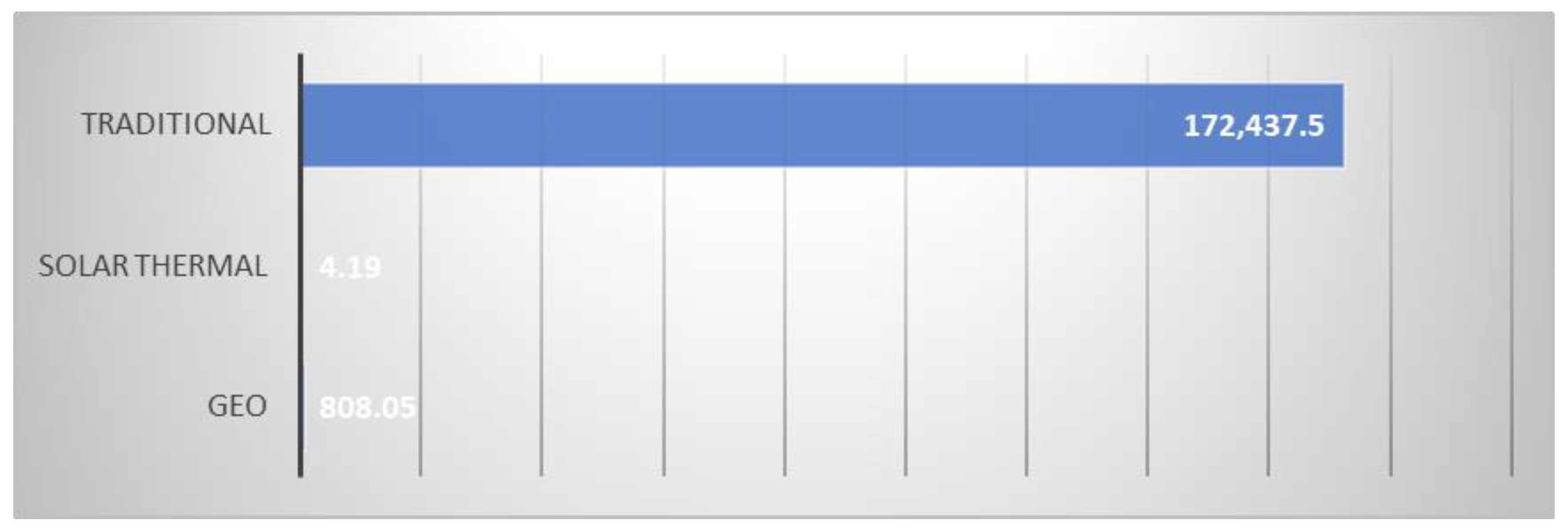
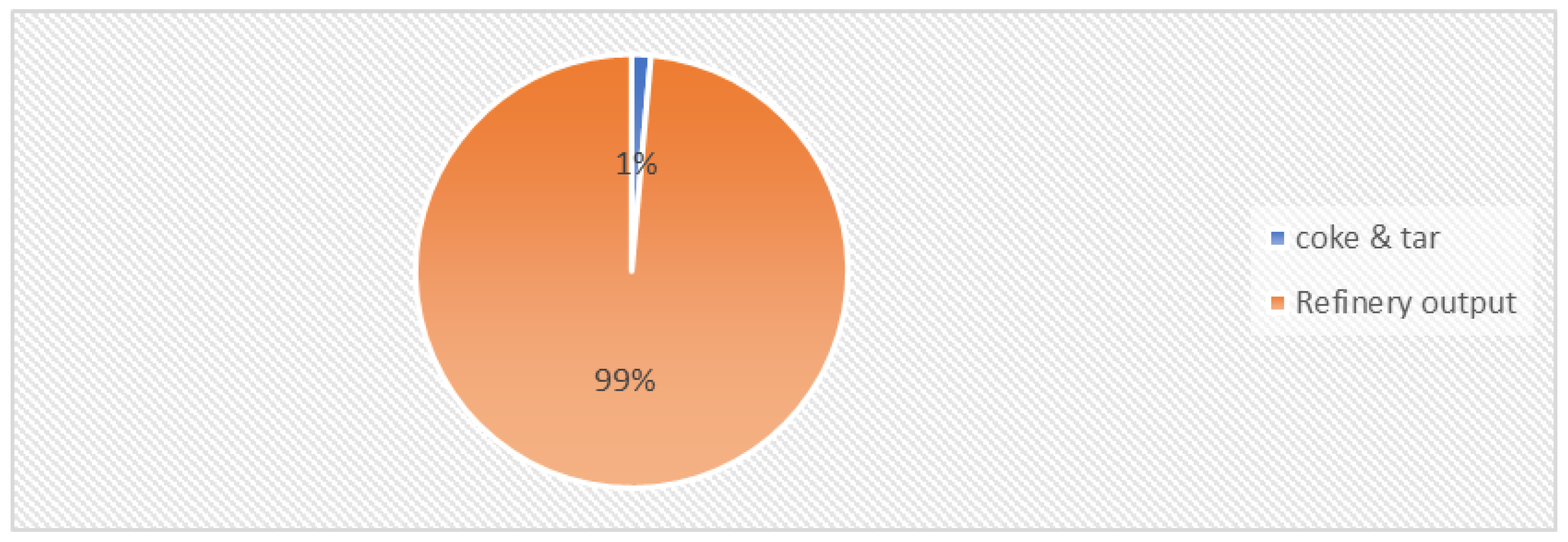
• CO converts the energy carriers from EX into heat and electrical energy with the generation of by-products (e.g., coke and refinery bottoms), thanks to contributions from DO, TR, and TE. Primary renewable energy inputs (solar, wind, geothermal, hydropotential) are “extracted” from the environment. The products are sent to TR, TE, and IN;
• IN generates consumer goods with added value. The products are dispatched to TE to be sold. Its inputs are EE fluxes from DO (workers), TR, and AG; energy from CO (distributed by TE); and raw materials from EX;
• AG receives exergy from DO, TE, TR, and the environment, generating semi-finished products to be sent to IN and in part to DO;
• DO supplies the labor force to all of the sectors, receiving goods and services from TE, TR, and partially from AG;
• TR receives refinery products from CO and labor from DO and supplies all of the sectors;
• TE provides goods and services to all of the sectors, receives the EE of CO and IN commodities, and sells them to DO and all of the other sectors (for example, electricity generated in CO is sold by utilities to all of the sectors, charged with their EE content due to the “production” of such an energy service). The exchanges with the other countries (“abroad”) represent import–export fluxes and are mediated in their entirety by TE.

2.2. Collecting Data

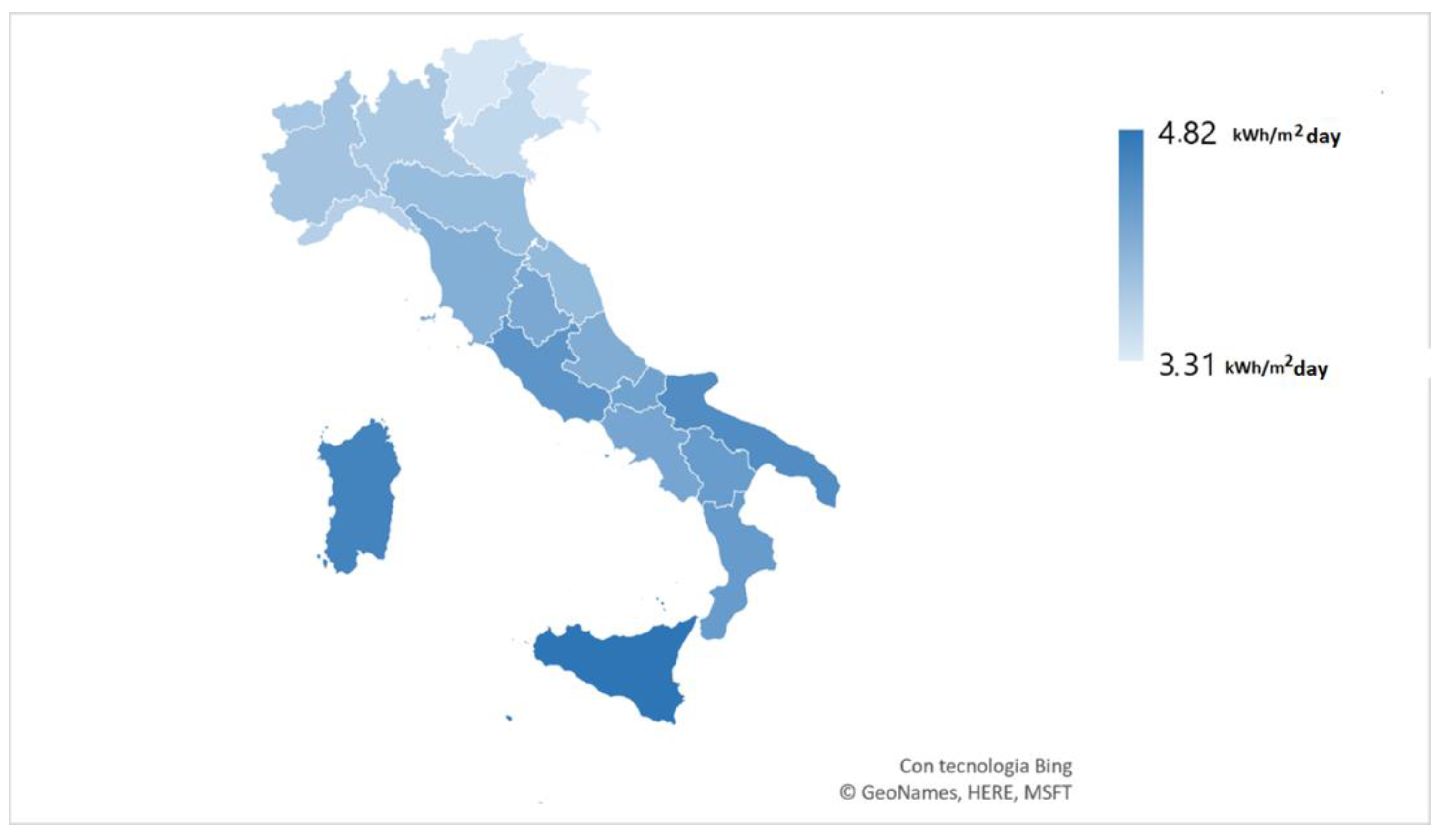
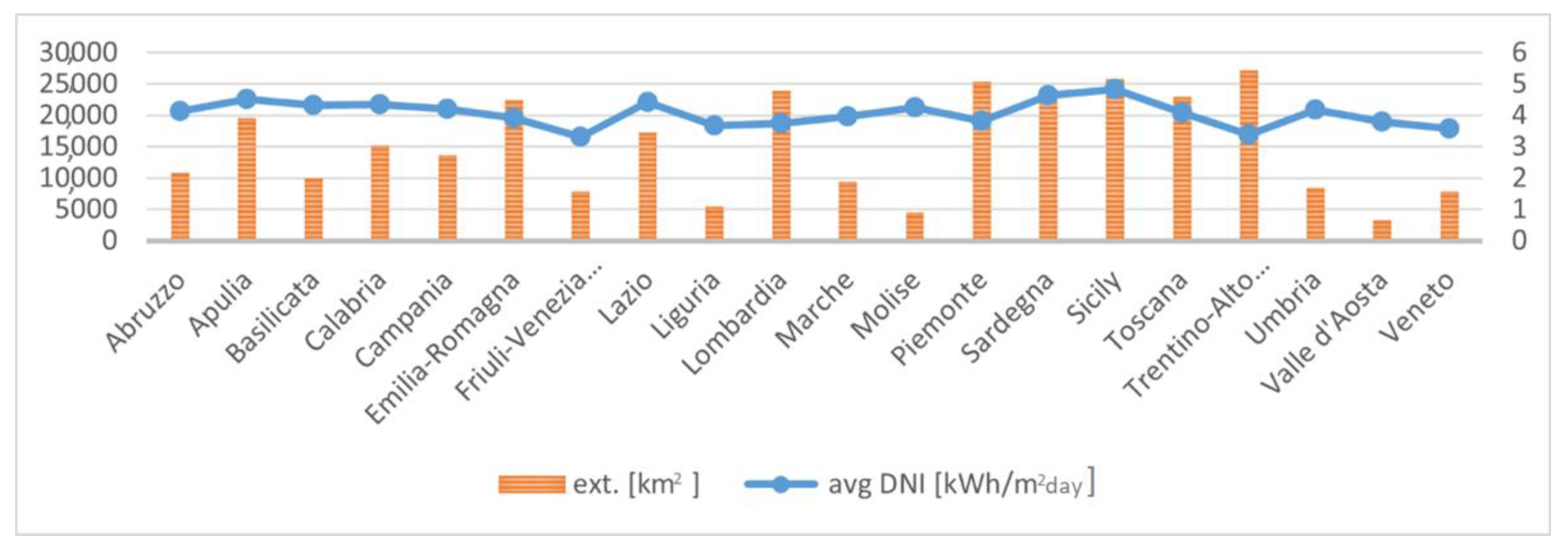
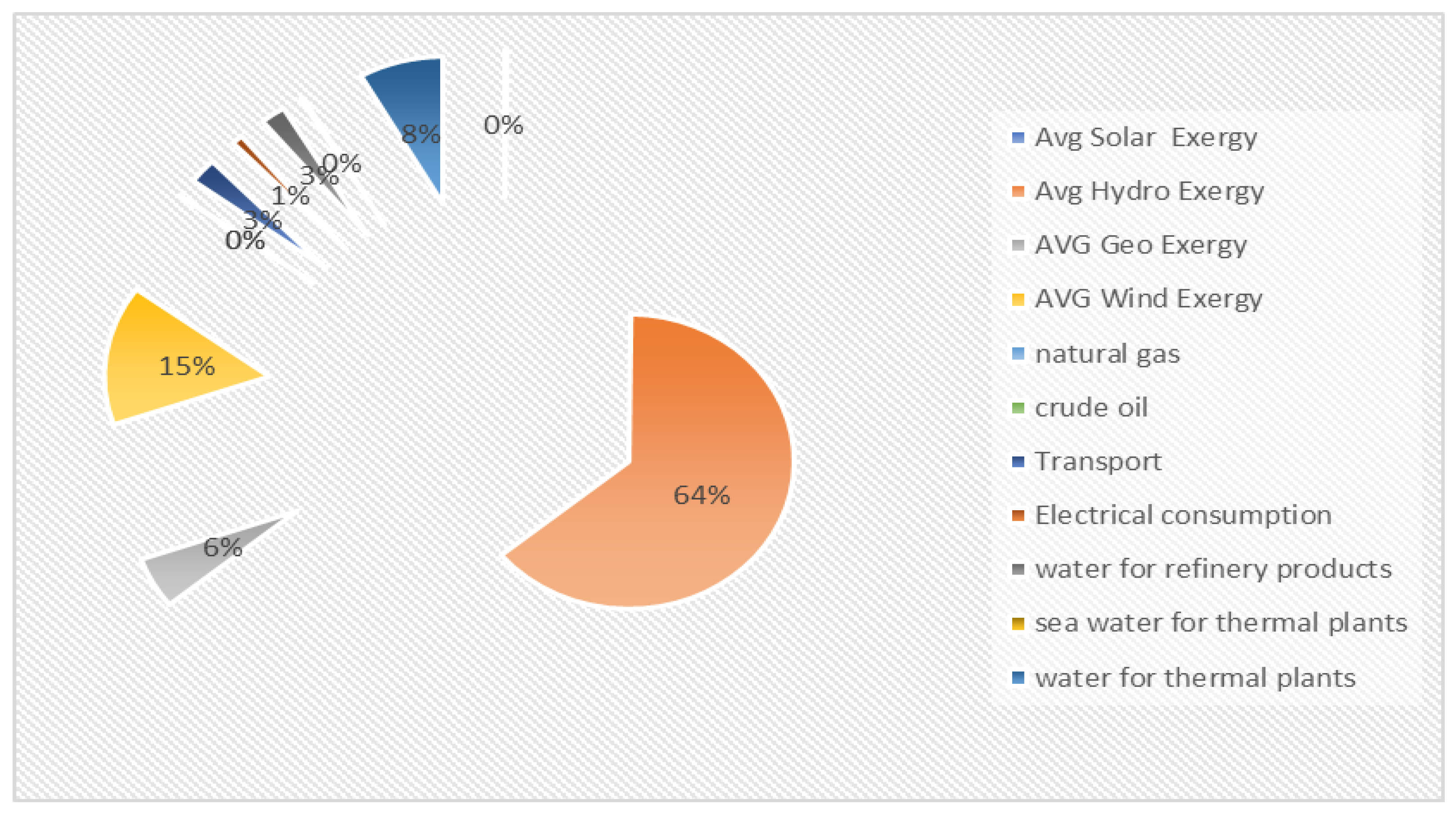
The stage of data collection shall define the detail of the model—the more disaggregated they are, the more credible the results but obviously the more complicated the collection, reconciliation, and organization. Data from different sources are structured in graphs and tables, from which it is possible to get insights that at first glance cannot be derived from their “raw” counterpart. In the future, this task might be left to specifically designed expert systems (knowledge-based methods). Here, we describe below the natural resources available for the Italian system.

2.2.1. Solar Exergy

Solar irradiation is obviously an input into AG. However, a portion of it feeds thermal and photovoltaic commercial and residential installations, so each energy stream associated with solar irradiation is allocated to each sector according to the data related to its consumption. Figure 2 shows the average direct normal irradiance (DNI) value and the surface extension of each region of Italy (data collected from [39,40]).

As illustrated in Figure 3, in Italy, as in most sub-tropical countries, the DNI distribution is not homogeneous, displaying a minimum value of 3.31 kWh/(m²day) in the northeast (Friuli-Venezia Giulia) and a peak of 4.82 kWh/(m²day) in the insular south (Sicily); for the sake of simplicity, a “representative” DNI value was obtained as a weighted mean of the regional values, using as the weight the surface extension of each region. The result is an average DNI for Italy of 4.01 kWh/(m²day) or 1461 kWh/(m²year). Assuming an average yearly temperature of 298 K, the ratio between solar exergy and energy equals 0.95 [29], thus the average exergy solar power value impinging on Italy equals the average DNI multiplied by the surface of the whole country multiplied by 0.95, which equals 1.60 × 10¹⁸ kJ/year.

2.2.2. Hydraulic Exergy Potential

To obtain an estimate of the exergy potentially extractable from the Italian waterways, the following procedure was adopted:

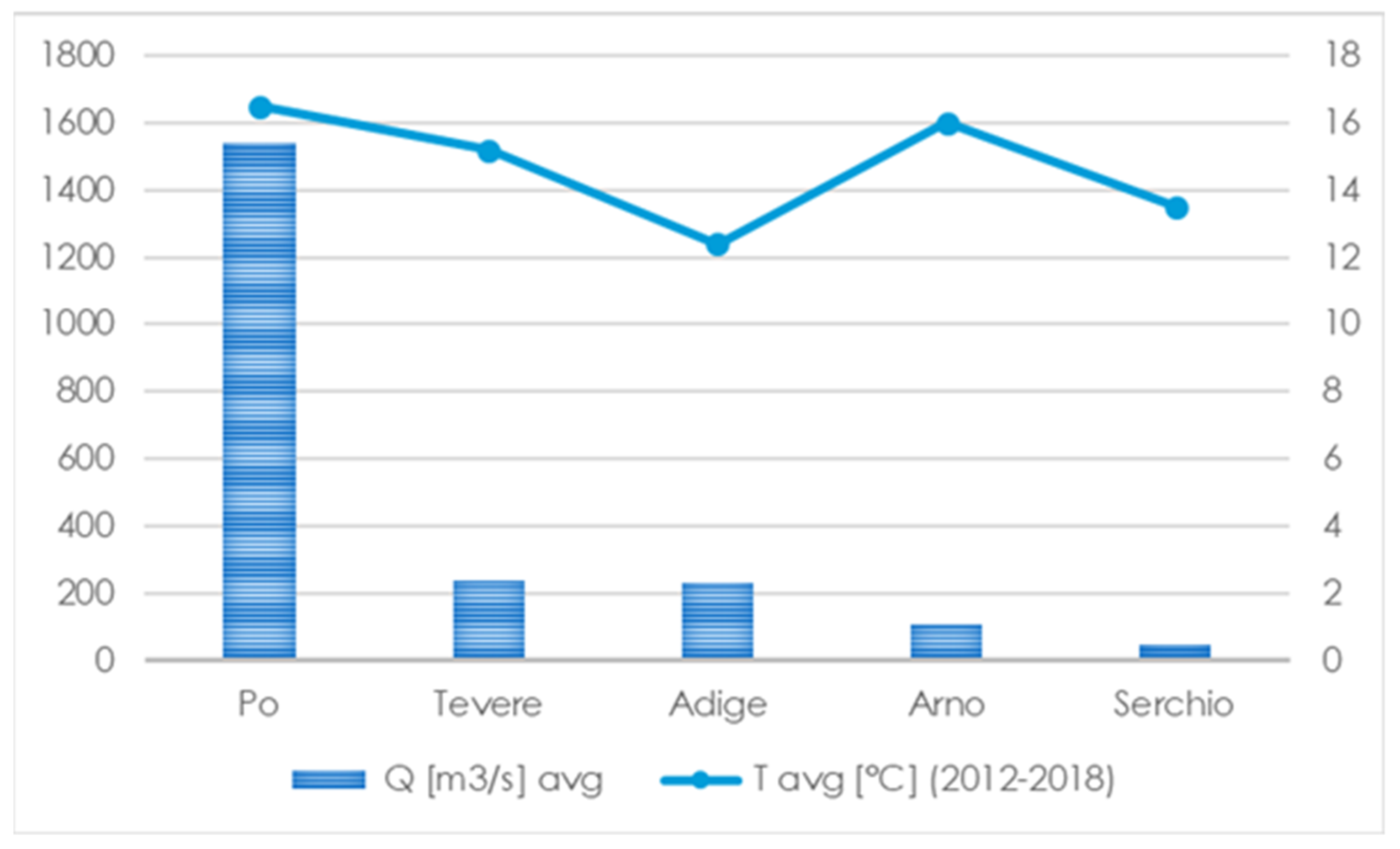
• From an orographic analysis of the Italian territory [41], the altitudes of the respective sources for the most important Italian rivers (Po, Tevere, Adige, Arno, Serchio) were derived;
• The flow rates of the rivers and their mean temperatures were collected (Figure 4) from a database for the period 2012–2018 [41,42,43,44,45,46], leading to a calculation of an average mass flow rate of 484 m³/s, with a mean temperature of 288.45 K;
• A mean temperature for the Italian seas was calculated as the average of the temperatures of the seas that bathe the Italian coasts;
• The equation developed by Valero et al. [47] was then used to compute the hydraulic-specific exergy of each river (neglecting the chemical exergy terms):

  $$e=C_p\left[T_p-T_0-T_{0}ln\frac{T_p}{T_0}\right]+gh [\mathrm{kJ}/\mathrm{kg}]$$

  (8)

  where e is the specific exergy associated with the waterways; c_p is the specific heat of the water at constant pressure, computed as an average value in the temperature range 15 to 20 °C [48]; T_p and T_o are the average temperature of the river and of the sea, respectively; g is the acceleration of gravity; and h is the average height. Equation (8) gives a specific exergy value; for the computation of power as outlined in [47], the following equation is proposed:

  $$E=Q·\rho ·e \left[\mathrm{kW}\right]$$

  (9)

  where Q is the average cumulative flow rate of the major Italian rivers; $\rho$ [48] is the density of water, computed as an average in the temperature range between 15 and 20 °C [48]; and e is the specific exergy computed using Equation (8). To obtain the final result of $2.73\times {10}^{15}$ kJ/year, the contributions resulting from Equation (9) for each river were summed; the results are summarized in

  Table 1. Results of the computation according to Valero’s model for the major Italian rivers [47].

  River	Q [m3/s] avg	T Avg [°C] (2012–2018)	et [kJ/kg]	ez [kJ/kg]	ew [kJ/kg]]	Ew [kJ·1015 Per Year]
  Po	1540	16.50	17.62	19.62	37.24	1.81
  Tevere	240	15.20	25.43	13.80	39.23	0.30
  Adige	235	12.40	42.37	15.21	57.58	0.43
  Arno	110	16.00	20.64	16.23	36.86	0.13
  Serchio	46	13.50	35.72	14.72	50.44	0.07

  . There are two caveats to be made here: first, the result measures the potential exergy, and thus friction losses and other factors are neglected (this makes the result somewhat overestimated); second, the myriad of smaller hydrological basins present in Italy (with potential power levels often lower than 1 MW) are neglected (which leads to an underestimated result). Both problems can be cured by using a more accurate (and costly in terms of human and computational resources) analysis approach.

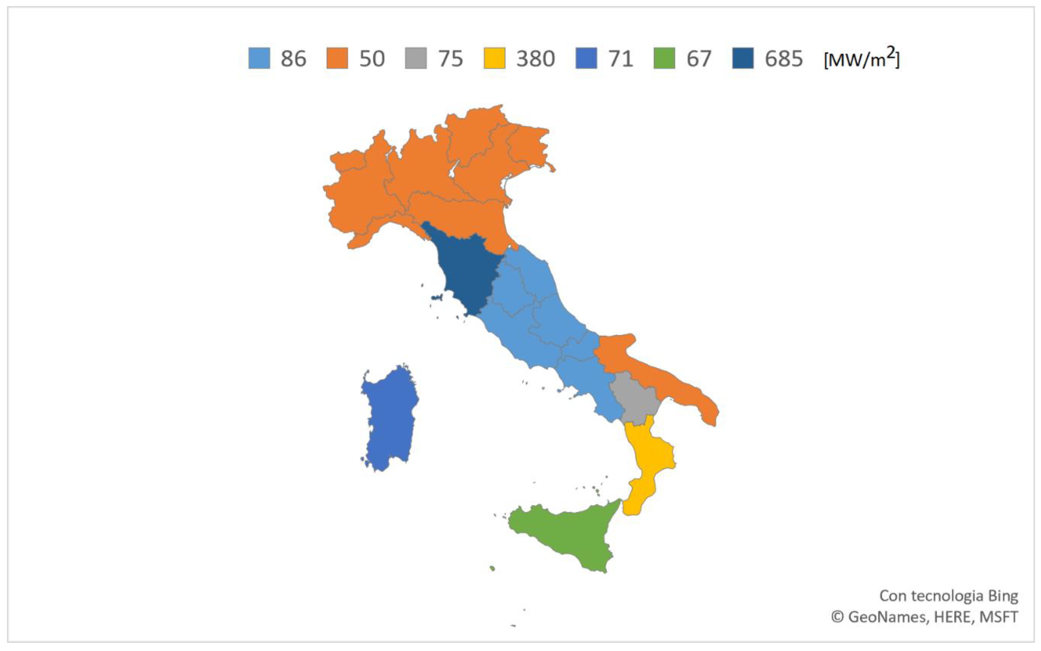
2.2.3. Geothermal Exergy

For the computation of geothermal exergy, the procedure was similar to that described above, using the data collected from [49]; the distribution of geothermal power is shown in Figure 5.

Again, the average geothermal energy is computed as a weighted average, with the weights being the extensions of each region. Considering the typical temperature ranges of the Italian sources (<150 °C), the potential geothermal exergy is computed by multiplying the average value of the corresponding energy by a Carnot factor of 0.25. The cumulative value equals $1.17\times {10}^{22}$ KJ/year.

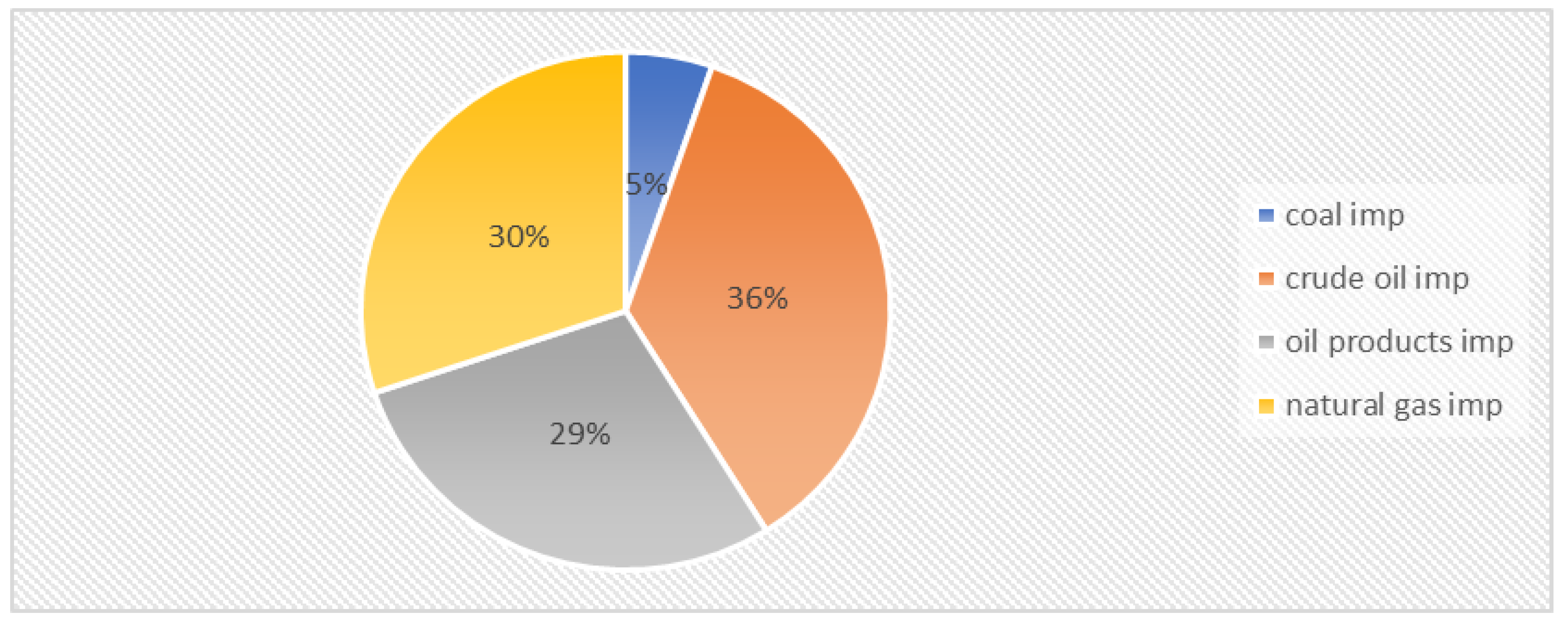
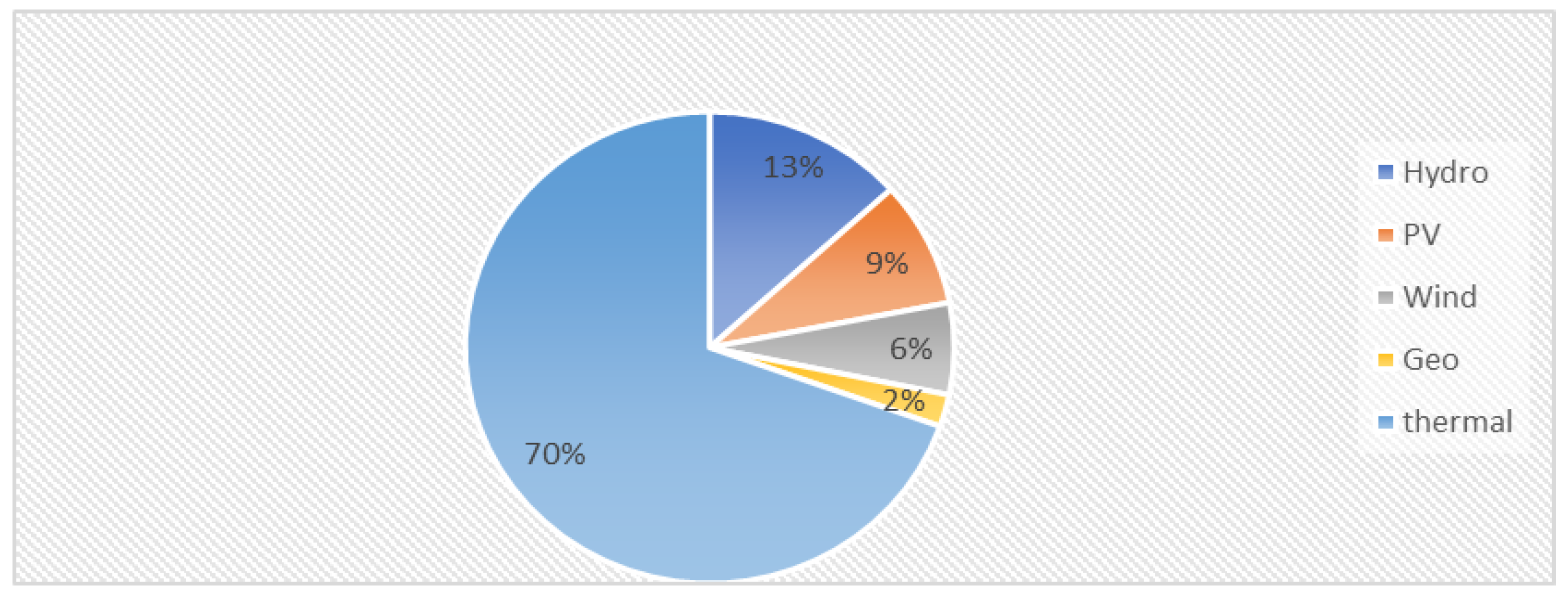
2.2.4. Other Material and Energy Flows

For the detection of the remaining material and energy flows, similar methods were adopted, with the details being omitted here for brevity. For each sector, several sources were consulted, including the national energy balance, material flow balance, clustered data on electricity and heat production as reported by the Italian National Statistics Institute (ISTAT) [50], the European Statistics Institute (EUROSTAT) [5], the national energy provider (TERNA_ [51,52], the national control unit of energy-related services (GSE) [53,54], and the Central Bank of Italy [55] (see reference list).

The window of observation spans 5 years, from 2013 to 2017 ([7,55,56,57,58,59,60,61,62,63]), whereby Δt is equal to 1 year.

2.3. Computation of the Econometric Factors and Specific Exergy of Labor and Capital

The econometric factors α and β were computed as follows [35]:

• The α factor measures the portion of the input exergy necessary for the survival of the population. This is computed as the ratio between the experimentally derived exergy flow into the domestic sector and the country’s total exergy input. Once α is known, the specific extended exergy of labor is computed as ${\mathrm{ee}}_{\mathrm{l}}=\frac{\mathsf{\alpha }•\mathrm{Ein}}{{\mathrm{N}}_{\mathrm{wh}}}$ where N_wh is the number of cumulative workhours per year;
• The second econometric factor, β, is also computed on the basis of experimentally derived data, namely the “money and quasi-money” aggregate M2 and the average salary Z; β is the ratio between M2 and the total average salary of a given year. From this perspective, β is a sort of amplification factor that produces wealth only from financial activities: the higher β is, the more the society is service-based. EEA introduces a systematic correction to this definition to take into account the so-called financial capital (the amount in excess of the global salaries in the country). The extended exergy embodied in one monetary unit is for a given year is computed as ${ee}_k=\frac{\mathsf{\alpha }·\mathsf{\beta }·{\mathrm{E}}_{in}}{\mathrm{M}2-Z}$.

3. Results and Discussion

Once the data were collected, organized, validated, and reconciliated, the extended exergy analysis of the Italian system for the period 2013–2017 was calculated. For simplicity, Figure 6, Figure 7, Figure 8, Figure 9 and Figure 10 show in a graphic form the input and output flows of a single sector, the CO sector. Notice the large number of flows, and therefore of the data involved; considering that other sectors like AG and IN are described by even more disaggregated data, they are not shown here so as not to burden the reading (they are available on www.exergyproject.unicusano.it). An important point is the very large amount of potential exergy available from the hydraulic source in Italy: this may suggest an investigation of this opportunity in more detail from a perspective of sustainable development, especially in view of the current trend of dismissing hydroplants of lower capacities on the ground of their low rate of return on investment (ROI). At the same time, this point reveals how such sources could be more effectively tapped, perhaps by a properly selected incentivizing campaign. The graphs related to the exergy output show an expected trend that might (and arguably must) change in the future; currently, the production of both electricity and thermal energy largely rely on traditional fossil systems, implemented in more or less standard thermal cycles (Rankine and Brayton cycles, often in a combined cycle configuration). Other insights from the analysis of the conversion sector for 2017 showed that production relies on carbon (completely imported) only for about 5% of the total, while (mostly imported) natural gas and (also imported) oil cover almost equal shares of the remaining 95%: unfortunately, this leads to a high dependence on the imports of these non-renewable energy carriers.

One of the aims of this study is to compute the amount of yearly exergy destruction of the Italian system to gain some insight into its correlation with the GDP. During their operation, each one of the 7 sectors destroys exergy, meaning the exergy budget for each sector will be:

$${\mathrm{EE}}_{\mathrm{IN}}{=\mathrm{EE}}_{\mathrm{OUT}}+\mathrm{E}{\delta }_{\delta }$$

(10)

The results of the analysis are shown in

Table 2. Results of the EE Analysis for Italy, 2013–2017. All data are shown in kJ·10¹².

2017	EIN (kJ·1012)	EOUT	Eδ	EEL	EEK	EE
AG	2905.90	1732.44	1173.46	400.45	18,640.86	21,947.21
EX	69.27	28.01	41.26	422.64	2.17	494.09
IN	4211.55	968.28	3243.27	131.01	6148.50	10,491.06
CO	8778.51	4724.16	4054.35	68.21	570,731.75	509,624.53
TE	12,463.94	10,697.22	1766.72	10.12	574,185.86	586,659.92
TR	1512.34	388.39	1123.96	3.47	160,136.96	161,652.77
DO	1649.77	1035.90	613.87	−1035.90	2968.49	3582.36
TOT	28,685.38	17,841.95	10,843.43	0.00	1,332,814.59	1,362,535.86
2016	EIN	EOUT	Eδ	EEL	EEK	EE
AG	2887.09	1779.23	1107.86	384.78	17,040.76	20,312.63
EX	73.33	32.03	41.29	406.11	1.97	481.41
IN	4947.39	939.42	4007.96	125.88	5499.02	10,572.29
CO	8415.80	4555.07	3860.73	65.54	499,290.95	507,772.29
TE	12,418.92	10,608.65	1810.27	9.72	562,765.64	575,194.29
TR	1460.26	401.69	1058.57	3.33	142,758.55	144,222.13
DO	1585.22	995.37	589.85	−995.37	2739.64	3329.49
TOT	31,788.01	19,311.47	12,476.54	0.00	1,230,096.53	1,261,884.53
2015	EIN	EOUT	Eδ	EEL	EEK	EE
AG	2940.42	1790.30	1150.12	458.25	19,907.85	23,306.51
EX	63.19	13.38	49.81	483.64	2.32	549.15
IN	4760.90	879.05	3881.85	149.92	5543.84	10,454.66
CO	8250.33	4693.21	3557.12	78.05	563,169.92	57,1498.30
TE	12,408.44	10,591.63	1816.80	11.58	634,644.77	647,064.79
TR	1484.77	426.98	1057.79	3.97	156,483.97	157,972.72
DO	1886.59	1185.41	701.18	−1185.41	2560.77	3261.95
TOT	31,794.63	19,579.96	12,214.67	0.00	1,382,313.43	1,414,108.07
2014	EIN	EOUT	Eδ	EEL	EEK	EE
AG	2960.82	2047.40	913.42	368.54	18263.90	21593.26
EX	61.95	20.39	41.56	388.96	2.12	453.04
IN	5168.07	862.21	4305.86	120.57	3606.89	8895.54
CO	8268.03	4493.09	3774.94	62.77	491,679.98	500,010.78
TE	12,017.59	10,678.87	133.72	9.31	498,016.78	510,043.68
TR	1512.74	413.24	1099.50	3.19	143,650.22	145,166.15
DO	1515.47	953.35	562.12	−953.35	2829.46	3391.58
TOT	31,504.67	19,468.55	12,036.13	0.00	115,8049.35	1,189,554.02
2013	EIN	EOUT	Eδ	EEL	EEK	EE
AG	2892.36	1991.91	900.44	400,758.53	18,416.43	21,709.55
EX	65.80	22.76	43.04	422964.83	2.30	491.07
IN	5382.00	949.04	4432.96	131,110.36	6703.98	12,217.09
CO	8317.61	4618.96	3698.66	68,260.19	529,971.34	538,357.22
TE	12,365.04	10,607.83	1757.21	10,127.29	597,372.91	609,748.08
TR	1456.88	400.68	1056.20	3469.77	144,359.58	145,819.93
DO	1651.03	1036.69	614.34	−1,036,690.96	2960.19	3574.53
TOT	32,130.72	19,627.87	12,502.85	0.00	1,299,786.73	1,331,917.46

.

The rationale behind the computation is the following: consider the connections between the sectors as described in Section 2.1 and, for the sake of clarity, let us examine in detail (albeit always at a schematic level) the exergy budget of the Industrial Sector IN (Figure 11, left). The sector is modelled as a black box: every exergy inflow represents a physical flow of either energy or matter and has a label expressing the units of specific exergy e_n [J/unit] and its intensity $\dot{m}$ or P [kg/s or kW], so that its total contribution to the IN exergy budget is calculated as $\dot{E}{ }_n$ = e_n*P or $\dot{E}{ }_m$= e_m*$\dot{m}$. By the same procedure, discarded material and energy flows provide the value of $\dot{E}{ }_w$. The accumulated exergy is calculated in the same way, on the basis of the bookkeeping of the tons of material stocked, the new constructions, possible accumulation in energy reservoirs, etc. The exergy budget never closes to zero, because a portion of the incoming exergy flows is unavoidably destroyed by irreversibilites. Since all outputs are also known, the exergy destruction is given (Equation (10) above) by the difference between the total input and the total output. Turning now to the extended exergy (Figure 11, right), it is clear that the cost of the output is necessarily equal to the sum of the cost of the inputs: each physical flow has an associated extended exergy $\dot{EE}$, but here the equivalent primary exergy costs of the externalities appear, calculated as described above. These are the capital flows ($\dot{E{E}_k}$= ee_K*K), labor (${\dot{EE}}_l$= ee_L*workhours) and environmental remediation (${\dot{EE}}_{env}$). The same applies to the remaining sectors: obviously, since the α and β coefficients depend on $\dot{E}{ }_{in}$ and $\dot{E}{ }_{consumed, Do}$, and the labor and capital flows depend in turn on the econometric coefficients, some iteration is necessary to reach convergence.

To use a formulation adopted by industrial economists, the extended exergy of a “stream”, be it material or immaterial, depends on 6 “production factors”: its initial CExC (material or immaterial), its labor content ${\dot{EE}}_l$, its capital content ${\dot{EE}}_{L K}$, its “added material” content ${\dot{EE}}_{L,M}$, its “added energy” content ${\dot{EE}}_{L,En}$ and its equivalent environmental remediation exergy ${\dot{EE}}_{L,ENV}$. This latter term is in practical terms difficult to calculate because it requires knowledge of the biodegradation process adopted: this will be not discussed here, interested readers are referred to [36]. It is therefore clear that the accuracy of an EEA analysis essentially depends on the quality (completeness, congruency) and detail (disaggregation) of the data. The following points summarize the results and the highlight the insights that emerge from the analysis of EE and E_δ and from a comparison with HDI, EF and BC and GDP trends. The EEA analysis shows that:

• The first econometric coefficient α is fairly constant over the time window of observation: it is equal to 4 × 10⁻⁴ and indicates that in spite of its high living standards, Italy is an “exergy sober” Country (values of α for different Countries for year 2005 are reported in [38]);
• The second econometric coefficient also remains fairly constant between 2013 and 2017: its values oscillate around 5.2. This indicates that Italy is a Country dominated by financial capital (K_f/Z = β − 1);
• The extended exergy of labor is a measure of how many joules i1 workhour is equivalent to—a higher ee_L pertains to more energy-intensive societies. The value for Italy did not change much from 2013 to 2017, being around 70 MJ/h;
• The extended exergy of capital is a measure of how many joules it takes to make up one monetary unit (€). A higher ee_K pertains to more affluent societies. The value for Italy did not change much from 2013 to 2017, being around 65 MJ/€;
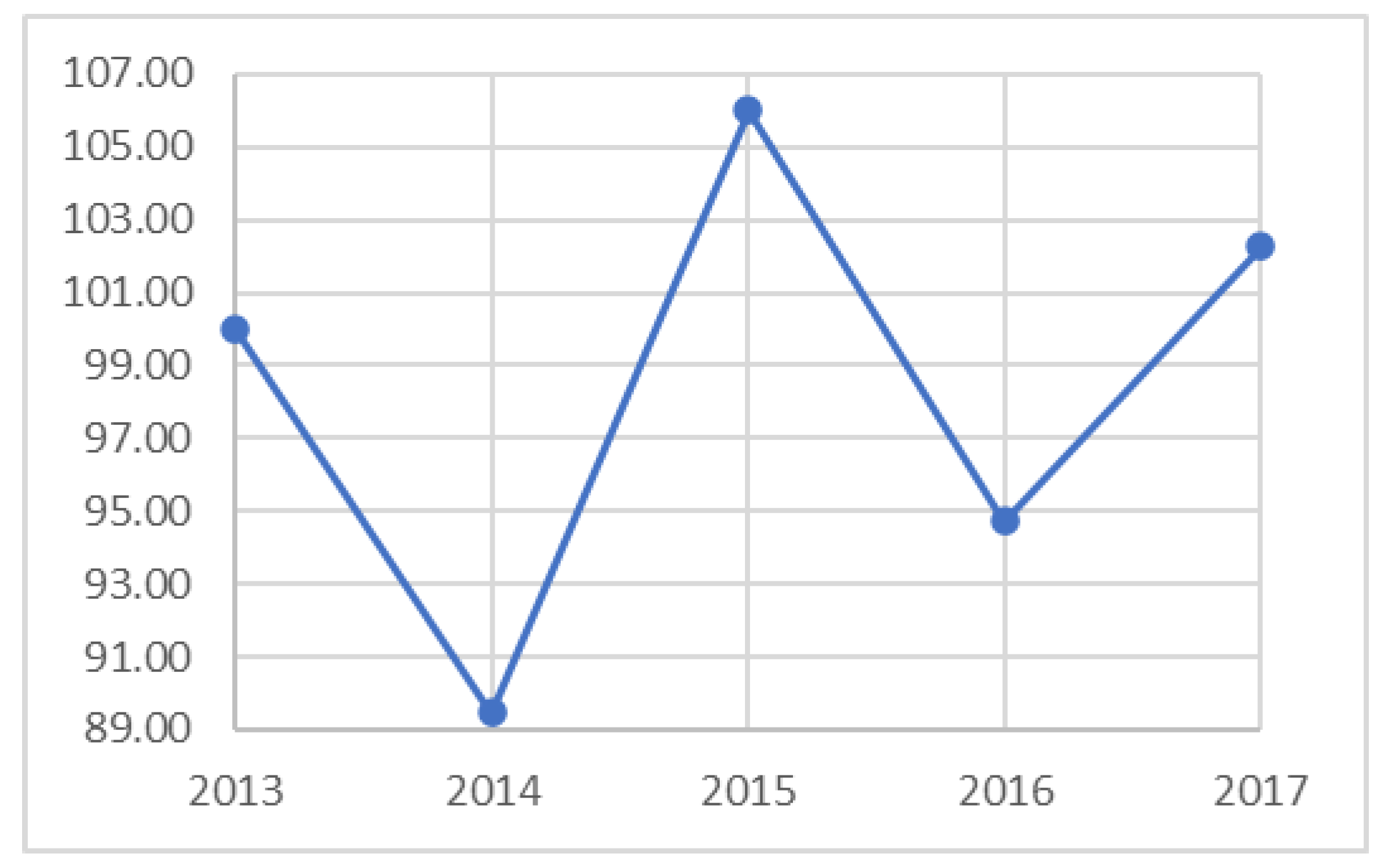
• The E_δ does not correlate with the GDP (Figure 12); considering the plots expressed as percentages of values for 2013, the GDP curve (Figure 13) was convex and growing, while the E_δ curve was fairly constant with variations that are below 5%, except for 2017, in which there was lower destruction (15% less compared to the value for 2013); this is an unexpected result worthy of further investigation;
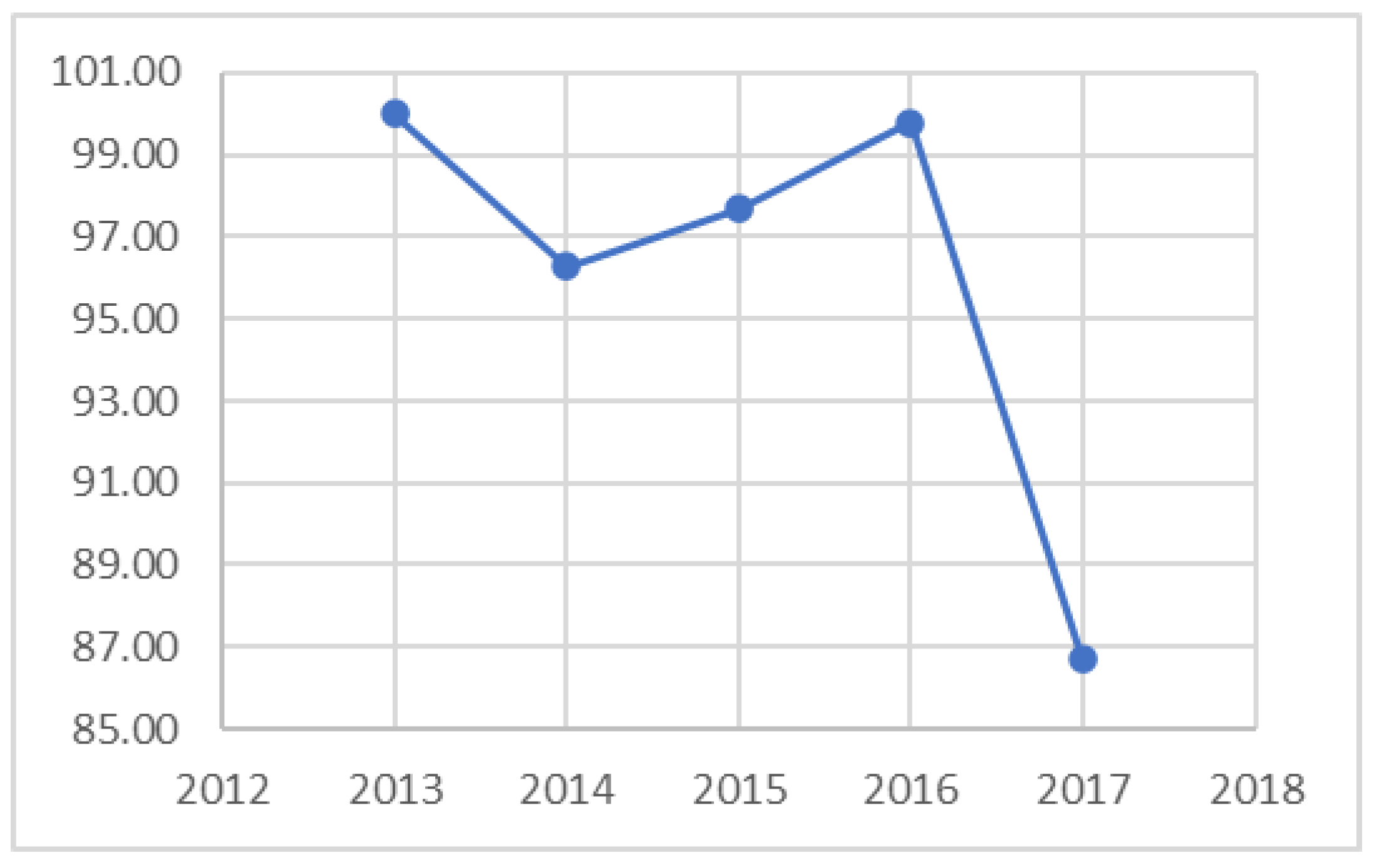
• The extended exergy (Figure 14), which is the “primary cost” of Italian society, is fairly constant, with an average value of around $1.31\times {10}^{18}$ kJ; the variations are with a range of ±10% with respect to the value for 2013. It is helpful to compare this trend with that from the GDP. Historically, we associate development and wellness with a growth of GDP, so considering Figure 14 one could be led to consider that Italian society is growing in “the right way”; the problem is that according to our analysis, the extended exergy of the country reached a plateau (Figure 14) with a maximum deviation w.r.t. the year 2013 of about 9% in 2014.This means that the “cost” of the economic and social growth remained constant throughout the years, highlighting the absence of progress with more rational exploitation of the available resources. In fact, this result suggests that the sustainability of the Italian society did not improve throughout the window of observation.

The possible insights that emerge from the analysis of EE and E_δ trends compared to those of the GDP, HDI, EF, BX, and Italian population for the period 2013–2017 are as follows:

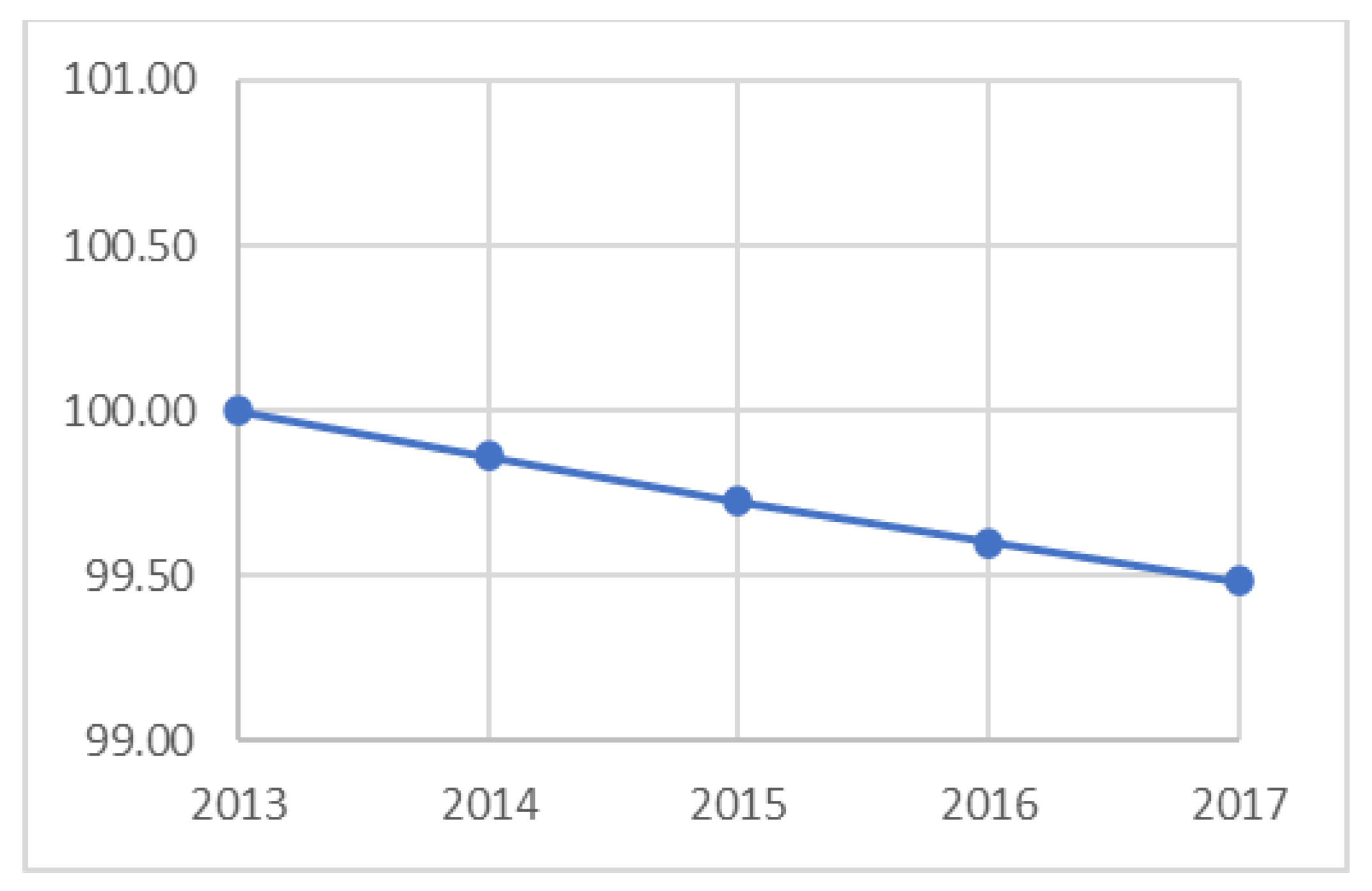
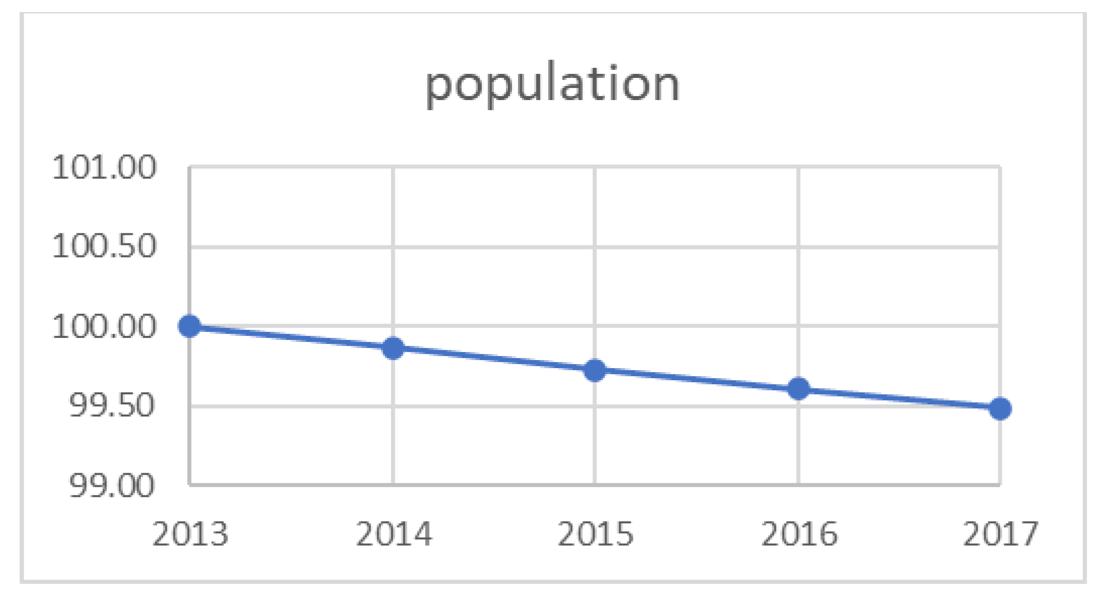
• The GDP grew exponentially from 2013 in the time frame considered, contrary to the trends for the HDI (Figure 15) and Italian population (Figure 16), whose variations compared to 2013 are hardly noticeable. This implies an increase in “wealth” but not in “wellness” (higher GDP pro capite but about the same HDI);
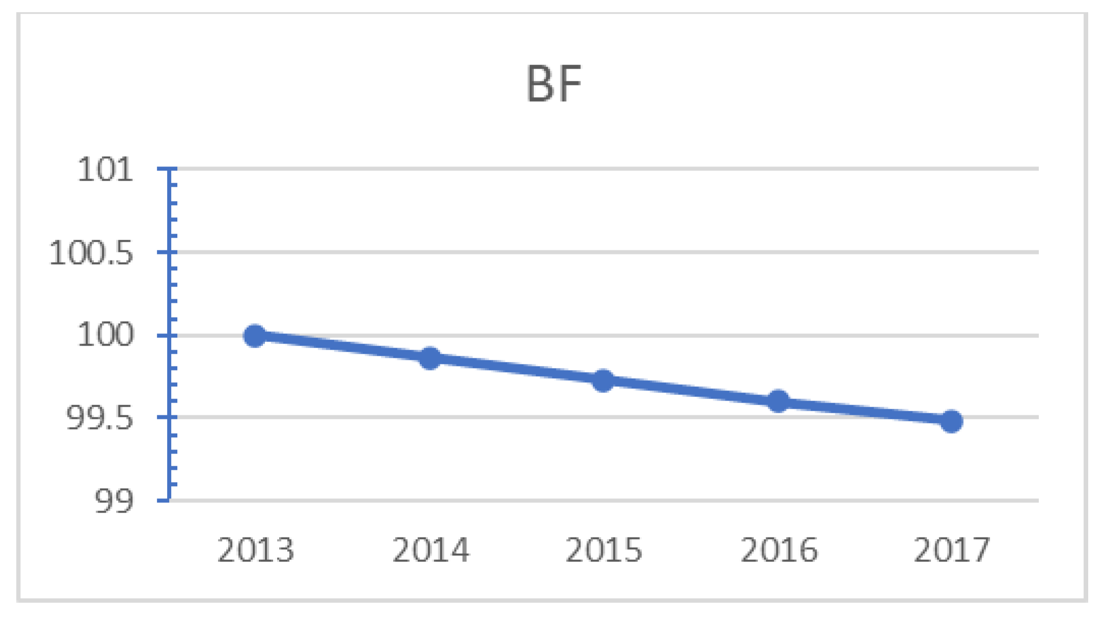
• It is worth noting that in spite of an increase in the pro capite domestic product and “wellness parameters” for HDI, the trends for EF (Figure 17) and BC (Figure 18) show that the EF is around 261 Pha, except for a lower value in 2014 (a trend well-correlated with EE), while there is a smooth decrease of BC, indicating an increase in the “ecological debt” of Italy;
• The trend for EE is similar to that of EF until 2015; from 2015 to 2017, the EF remains pretty constant, while the EE decreases in 2016 and increases in 2017. This could suggest that the “cost” of Italian wellness was obtained at the expense of the non-renewable sources, which are not considered in the EF accounting. This calls for a more detailed analysis of the reasons for the increase of EE. This might well be due to less sustainable development that is not evidenced by other sustainability indicators.

4. Conclusions

An extended exergy analysis of the Italian system was conducted over a period of five years (2013–2017). This EEA analysis was based on the most disaggregated database used to date. An innovative data validation and reconciliation procedure was implemented to assure the full congruency of the data prior to the actual analysis. The Italian society was divided into the usual 7 sectors, plus the environment sector and a virtual sector (“abroad”), which accounted for the import and export of materials and energy fluxes. The two econometric coefficients α and β or the quantification of the extended exergy were calculated for each year on the basis of public domain statistical data and then used to calculate the specific extended exergy of labor ee_L and of capital ee_K. All values are consistent with previous analyses and confirm the validity of the current approach. The exergy destruction in the system and the extended exergy are compared with the GDP across the observation window, and it clearly appears that the two are not correlated. The study also includes a first-order comparison with other indicators (HDI, EF, BC, and the Italian population) to derive “differentials” that could be suggestive of the sustainable development of the country. It is likely that separate, more accurate analyses of each sector are necessary to validate the results; since the accuracy depends on the disaggregation of the available data, this task is left for future studies. It is worth noting that each different indicator focuses its attention on specific aspects of a society, namely economic, social, or related to renewable intensity. A comparison of their trends over the same time period suggests that the current policy, which incentivizes the use of renewables (thus leading to a decrease of the EF), is still somewhat too timid, in that it still substantially relies on the tapping of non-renewable sources. This is indicated by the decreasing trend of EE, which is not reflected in a corresponding decrease of the EF. The potential usefulness of the application of EEA to a society lies in the possibility of analyzing the policies of a government by considering both energy and economic production factors. Italy’s economy is tertiary-dominated, as witnessed by its high value of the financial amplification factor β (which had average values of around 5 throughout the observation window), resulting in a relatively high value for the EE of capital. As a suggestion for policymakers, it may be concluded that since the country EE is surely affected by economic factors such as K_f and the financial capital (i.e., the excess of the monetary circulation over the total amount of the wage capital S), and also relies strongly on the final energy use mix (ratio of the exploitation of renewable and non-renewable sources) and on the allocation of soil use, the status quo confirms a strong dependence of Italy on materials and energy imports from abroad. An EEA makes it possible to condense all of this information into one single parameter, resulting in a very useful decision support tool to evaluate the health of a country and to compare possible future scenarios.

References

1. United Nations Department of Economic and Social Affairs, Population Division (DESA). The 2019 Revision of World Population Prospects; DESA: New York, NY, USA, 2019. [Google Scholar]
2. SDSN & IEEP. The 2019 Europe Sustainable Development Report. Sustainable Development Solutions Network and Institute for European Environmental Policy: Paris and Brussel; IEEP: Bruxelles, Belgium, 2019. [Google Scholar]
3. Dynan, K.; Sheiner, L. GDP as a Measure of Economic Well-Being. Work. Pap. 2018, 43. [Google Scholar]
4. Costanza, R.; Maureene, H.; Posner, S.; Talberth, J. Beyond GDP: The Need for New Measures of Progress. Pardee Pap. 2009, 4, 1–46. [Google Scholar]
5. Ivkovič, A.F. Limitations of the GDP as a Measure of Progress and Well-Being. Econviews 2016, 29, 257–272. [Google Scholar]
6. Stanton, E.A. The Human Development Index: A History; Political Economy Research Institute (USA): Amherst, MA, USA, 2007. [Google Scholar]
7. Schaefer, F.; Luksch, U.; Steinbach, N.; Cabeça, J.; Hanauer, J. Ecological Footprint and Biocapacity-The World’s Ability to Regenerate Resources and Absorb Waste in a Limited Time Period; The Publications Office of the European Union: Luxemburg, 2006. [Google Scholar]
8. Subjective Well-Being. Available online: https://www.eurofound.europa.eu/it/topic/subjective-well-being (accessed on 3 March 2020).
9. Santos, M.E.; Alkire, S. Training Material for Producing National Human Development Reports; Oxford Poverty & Human Development Initiative (OPHI): Oxford, UK, 2015. [Google Scholar]
10. WWF Living Planet Report. Available online: https://livingplanet.panda.org (accessed on 4 March 2020).
11. Empresa, P.E.; Rio, J. Brazilian Energy Balance 2008-year 2007. Braz. Energy Balance 2008, 43, 37. [Google Scholar]
12. Eurostat. Available online: https://ec.europa.eu (accessed on 8 December 2020).
13. Energy Balance of Italy. Available online: https://dati.istat.it (accessed on 8 December 2020).
14. Abele, E.; Beckmann, B. Energieeffizienzsteigerung von Fabriken. Z. Wirtsch. Fabr. 2012, 107, 261–265. [Google Scholar] [CrossRef]
15. Rocco, M.; Colombo, E.; Sciubba, E. Advances in exergy analysis: A novel assessment of the Extended Exergy Accounting method. Appl. Energy 2014, 113, 1405–1420. [Google Scholar] [CrossRef]
16. Wall, G. Exergy conversion in the Swedish society. Resour. Energy 1987, 9, 55–73. [Google Scholar] [CrossRef] [Green Version]
17. Wall, G. Exergy conversion in the Japanese society. Energy 1990, 15, 435–444. [Google Scholar] [CrossRef]
18. Hammond, G.P.; Stapleton, A.J. Exergy analysis of the United Kingdom energy system. Proc. Inst. Mech. Eng. 2001, 215, 141–162. [Google Scholar] [CrossRef]
19. Ertesvåg, I.S. Society exergy analysis: A comparison of different societies. Energy 2001, 26, 253–270. [Google Scholar] [CrossRef]
20. Brockway, P.E.; Barrett, J.R.; Foxon, T.J.; Steinberger, J.K. Divergence of Trends in US and UK Aggregate Exergy Efficiencies 1960–2010. Environ. Sci. Technol. 2014, 48, 9874–9881. [Google Scholar] [CrossRef]
21. Chen, B.; Chen, J.Q. Exergy Analysis for Resource Conversion of the Chinese Society 1993 Under the Material product System. Energy 2006, 31, 1115–1150. [Google Scholar] [CrossRef]
22. Koroneos, C.J.; Nanaki, E.A. Energy and Exergy utilization Assessment of the Greek Transoprt Sector. Resour. Conserv. Recycl. 2008, 52, 700–706. [Google Scholar] [CrossRef]
23. Dai, J.; Chen, B.; Sciubba, E. Extended Exergy Based Economic Accounting for the Transportation Sector in China. Renew. Sustain. Energy Rev. 2014, 32, 229–237. [Google Scholar] [CrossRef]
24. Sciubba, E.; Bastianoni, S.; Tiezzi, E. Exergy and extended exergy accounting of very large complex systems with an application to the province of Siena, Italy. J. Environ. Manag. 2008, 86, 372–382. [Google Scholar] [CrossRef] [PubMed]
25. Ertesvag, I. Energy, exergy, and extended-exergy analysis of the Norwegian society 2000. Energy 2005, 30, 649–675. [Google Scholar] [CrossRef]
26. Ptasinski, K.; Koymans, M.; Verspagen, H. Performance of the Dutch Energy Sector based on energy, exergy and Extended Exergy Accounting. Energy 2006, 31, 3135–3144. [Google Scholar] [CrossRef]
27. Biondi, A.; Sciubba, E. New Insights from Econometric Data: An Extended Exergy Analysis (EEA) of the Italian System, 2013–2017. Proceedings 2020, 58, 3. [Google Scholar] [CrossRef]
28. Feynman, R.P.; Leighton, R.B.; Sands, M.; Hafner, E.M. The Feynman Lectures on Physics. Am. J. Phys. 1965, 33, 750–752. [Google Scholar] [CrossRef]
29. Petela, R. Engineering Thermodynamics of Thermal Radiation; McGrawHill: New York, NY, USA, 2010. [Google Scholar]
30. Szargut, J.; Ziębik, A.; Stanek, W. Depletion of the Unrestorable Natural Exergy Resources as a Measure of the Ecological Cost. Energy Convers. Manag. 2002, 42, 1149–1163. [Google Scholar] [CrossRef]
31. Szargut, J.; Morris, D.R.; Steward, F.R. Exergy Analysis of Thermal, Chemical, and Metallurgical Processes; Hemispere Pub.: New York, NY, USA, 1988. [Google Scholar]
32. Valero, A.; Usón, S.; Torres, C.; Valero, A. Application of Thermoeconomics to Industrial Ecology. Entropy 2010, 12, 591–612. [Google Scholar] [CrossRef]
33. Sciubba, E. A novel exergetic costing method for determining the optimal allocation of scarce resources. In Proceedings Contemporary Problems of Thermal Engineering; Ziebek, A., Ed.; Springer: Gliwice, Poland, 1998; pp. 311–324. [Google Scholar]
34. Sciubba, E. Beyond thermoeconomics? The concept of Extended Exergy Accounting and its application to the analysis and design of thermal systems. Exergy Int. J. 2001, 1, 68–84. [Google Scholar] [CrossRef]
35. Sciubba, E. A revised calculation of the econometric factors α- and β for the Extended Exergy Accounting method. Ecol. Model. 2011, 222, 1060–1066. [Google Scholar] [CrossRef]
36. Yumashev, A.; Ślusarczyk, B.; Kondrashev, S.; Mikhaylov, A. Global Indicators of Sustainable Development: Evaluation of the Influence of the Human Development Index on Consumption and Quality of Energy. Energies 2020, 13, 2768. [Google Scholar] [CrossRef]
37. Barret, J.; Cherret, N.; Birch, R. Exploring the application of the Ecological Footprint to Sustainable Consumption Policy. J. Environ. Policy Plan. 2005, 7, 234–247. [Google Scholar] [CrossRef]
38. Lin, D.; Hanscom, L.; Murthy, A.; Galli, A.; Evans, M.; Neill, E.; Mancini, M.S.; Martindill, J.; Medouar, F.; Huang, S.; et al. Ecological Footprint Accounting for Countries: Updates and Results of the Nationals Footprint Accounts, 2012–2018. Resources 2018, 7, 58. [Google Scholar] [CrossRef] [Green Version]
39. Global Solar Atlas. Available online: http://globalsolaratlas.info (accessed on 3 February 2020).
40. ISTAT. La Superficie dei Comuni, delle Province e delle Regioni Italiane; ISTAT: Rome, Italy, 2013.
41. Ministero della Transizione Ecologica. Available online: http://miniambiente.it (accessed on 3 February 2020).
42. Autorità del Bacino del Fiume Adige. Available online: http://bacino-adige.it (accessed on 3 March 2020).
43. Agenzia Regionale per la Protezione Ambientale Toscana. Available online: http://arpat.toscana.it (accessed on 3 March 2020).
44. Agenzia Regionale per la Protezione Agenzia Regionale per la Protezione Veneto. Available online: http://www.arpa.veneto.it (accessed on 3 March 2020).
45. Autorità Bacino Fiume Serchio. Available online: http://autorita.bacinoserchio.it (accessed on 3 March 2020).
46. Bacino idrografico Regione Lazio. Available online: http://idrografico.regione.lazio.it (accessed on 3 March 2020).
47. Valero, A.; Valero, A.; Martínez, A. Physical Hydronomics: Application of the exergy analysis to the assessment of environmental costs of water bodies. The case of the inland basins of Catalonia. Energy 2009, 34, 2101–2107. [Google Scholar] [CrossRef]
48. National Institute of Standards and Technology. Available online: http://webbook.nist.gov (accessed on 5 March 2020).
49. Davies, J.H. Global map of solid Earth surface heat flow. Geochem. Geophys. Geosyst. 2013, 14, 4608–4622. [Google Scholar] [CrossRef]
50. Data Bank Italian Statistics Institute. Available online: http://dati.istat.it (accessed on 5 March 2020).
51. TERNA. Produzione e Richiesta di Energia Elettrica in Italia dal 1883 al 2018; TERNA: Brussels, Belgium, 2019. [Google Scholar]
52. TERNA. Consumi Energia Elettrica in Italia; TERNA: Brussels, Belgium, 2019. [Google Scholar]
53. Gestore dei servizi energetici (GSE). Energia nel Settore Trasporti 2005–2018; GSE: Rome, Italy, 2019. [Google Scholar]
54. Gestore dei servizi energetici (GSE). Rapporto Statistico FER 2017; GSE: Rome, Italy, 2018. [Google Scholar]
55. Available online: www.bancaditalia.it. (accessed on 4 March 2020).
56. ISTAT. Censimento Generale Dell’agricoltura-Utilizzo Della Risorsa Idrica a Fini Irrigui in Agricoltura; ISTAT: Rome, Italy, 2014.
57. ISTAT. Utilizzo e Qualità della Risorsa Idrica in Italia; ISTAT: Rome, Italy, 2019.
58. Note, A.; Collalti, A.; Borghetti, M.; Chiesi, M. The Role of Managed Forest Ecosystems: A Modelling Based Approach, Environmental Science and Engineering; Springer: Berlin/Heidelberg, Germany, 2014. [Google Scholar]
59. Istituto Superiore per la Protezione e la Ricerca Ambientale. Available online: http://isprambiente.gov.it (accessed on 5 March 2020).
60. Istituto Superiore per la Protezione e la Ricerca Ambientale (ISPRA). Il Piombo Nelle Munizioni da Caccia: Problematiche e Possibili Soluzioni; ISPRA: Roma, Italy, 2012.
61. Sharqawy, M.H.; Zubair, S.M. On exergy calculations of seawater with applications in desalination systems. Int. J. Therm. Sci. 2011, 50, 187–196. [Google Scholar] [CrossRef]
62. Human Development Reports. Available online: http://hdr.undp.org/en/countries/profiles/ITA (accessed on 24 January 2020).
63. Open Data Platform. Available online: https://data.footprintnetwork.org/#/ (accessed on 24 January 2020).
Figure 1. Qualitative scheme of different material (M), energy (E), monetary (K), and labor (L) flows among the different sectors (schematic: not all flow types are shown).
Energies 14 02767 g001
Figure 2. Distribution of yearly averaged DNI in Italy. Adapted from [39].
Energies 14 02767 g002
Figure 3. Average DNI for Italian regions vs. their extension.
Energies 14 02767 g003
Figure 4. Flow rates of some of the major Italian rivers vs. their mean temperatures between 2012 and 2018.
Energies 14 02767 g004
Figure 5. Distribution of geothermal power in the Italian territory. Elaboration of data from [49].
Energies 14 02767 g005
Figure 6. Exergy inputs of the Italian CO sector according to the proposed EE model (2017 data).
Energies 14 02767 g006
Figure 7. Exergy inputs of the Italian CO sector, including imports and exports (2017 data).
Energies 14 02767 g007
Figure 8. Exergy outputs of the Italian CO sector according to production technology. Hydro and thermal cycles (Rankine and Brayton cycles) still lead the sector (2017).
Energies 14 02767 g008
Figure 9. Exergy outputs of the CO sector [TJ]: heat production. The use of traditional sources (fossil fuels) dominates the sector (2017).
Energies 14 02767 g009
Figure 10. Exergy outputs of by-products of the CO sector (2017).
Energies 14 02767 g010
Figure 11. Black box model of the industrial sector within the context of an exergy analysis (left) and extended exergy analysis (right).
Energies 14 02767 g011
Figure 12. The 2013–2017 exergy destruction in Italy. For the 2013 value, 1252.85 × 1012 kJ is set to 100%.
Energies 14 02767 g012
Figure 13. GDP growth in percentage w.r.t. to the 2013 value.
Energies 14 02767 g013
Figure 14. Extended exergy from 2013 to 2017. The 2013 value (1331917.46) is set to 100%.
Energies 14 02767 g014
Figure 15. HDI trend as a percentage of its 2013 value.
Energies 14 02767 g015
Figure 16. Italian population growth trend from 2013 to 2017. The 2013 value (59701104) is set to 100%.
Energies 14 02767 g016
Figure 17. Ecological footprint from 2013 to 2017. Percentage values refer to 2013 (EF2013= 262.68 Pha).
Energies 14 02767 g017
Figure 18. Biocapacity trend from 2013 to 2017. Percentage values refer to 2013.
Energies 14 02767 g018