Minimum Set of Rotor Parameters for Synchronous Reluctance Machine and Improved Optimization Convergence via Forced Rotor Barrier Feasibility ^†

Abstract

Although rare earth materials are the critical component in high torque density permanent magnet machines, their use has historically been a commercial risk. The alternatives that have been in the recent industry focus are synchronous reluctance machines (SyRM). They have lower torque density but also relatively low material cost and higher overload capability. Multi-layer IPM and SyRM machines have significant geometric complexity, resulting in a high number of parameters. Considering that modern machine design requires the use of optimization algorithms with computational load proportional to the number of parameters, the whole design process can take several days. This paper presents novel SyRM parameterization with reduced number of parameters. Furthermore, the paper introduces the novel forced feasibility concept, applied on rotor barrier parameters, resulting in improved optimization convergence with overall optimization time reduced by 12.3%. Proposed approaches were demonstrated using optimization procedure based on the existing differential evolution algorithm (DE) framework.

1. Introduction

To reduce environmental impact, global legislation is pushing to increase electric vehicle (EV) production [1]. In addition to regulatory requirements, consumers are demanding cleaner and safer vehicles. This has led to a tectonic shift in the automotive industry, both in terms of knowledge and production, forcing the industry to evolve rapidly.

At the moment, passenger vehicles are leading the market development (Tesla, Toyota, BMW), mainly because of lighter vehicles that require smaller traction batteries. On the other hand, commercial vehicles are much heavier and require large battery capacity, resulting in significant production costs. Therefore, the commercial vehicle industry is forced to move into niche markets, such as medium-duty, short-haul, and last mile applications. Long-haul vehicle development is likely to take more time and have even more sensitive financing.

Examples of commercial vehicles suitable for SyRM adoption include electric multi-purpose vehicles (eMPVs), such as refuse trucks, hook loader trucks, or vacuum trucks [2]. eMPVs must actuate additional body systems (usually through some type of hydraulic pump) in addition to electric propulsion. Traditionally, this actuation is done by a diesel engine or a gearbox-mounted output shaft referred to as power take-off (PTO). Considering price, overload capability, and production simplicity, SyRM can be a viable ePTO solution [2,3].

This paper presents novel SyRM parameterization with a reduced number of parameters (rotor nomenclature according to Figure 1). During the optimization process, infeasible models may occur. Depending on the designer’s choice, the infeasible models can be rejected or modified until they become feasible. The idea is that the procedure does not discard randomly generated infeasible geometry but modifies it until feasibility is achieved (hence the name “forced” feasibility).

2. SyRM Design

2.1. Peak Performance Requirements

The machine requirements in this paper are derived from Reference [3]. All peak performance requirements are listed in

Table 1. Peak operation requirements at base speed.

Description	Symbol	Value	Unit
Base speed	$n_b$	1700	rpm
Max. operating speed	$n_{\max }$	2500	rpm
Max. over speed	$1.2·n_{\max }$	3000	rpm
Max. torque	$T_{\max }$	600	Nm
Battery voltage	$U_{\mathrm{DC}}$	610	V
Max. phase current	$I_{\mathrm{s}\max }$	310	Arms
RMS current density	J	18.4	A/mm2

.

2.2. Optimization Method

Most of the requirements for the design of electrical machines are in conflict with each other (reduction of volume or mass, increase of efficiency, etc.). This is evident in the problem of increasing efficiency [4,5,6] through global legislative initiatives [1]. For traction drives, high efficiency in limited packaging space is an absolute imperative [7]. Therefore, a manual design that satisfies all constraints can be an overwhelming task due to a large number of coupled parameters that affect the performance and quality of the machine.

According to Pellegrino [8,9], the computational load increases proportionally with the number of geometric parameters. This is inherently the case for IPM and SyRM machines, leading to a high number of optimization variables and a longer optimization time.

Today, optimization algorithms enjoy great popularity among designers of electrical machines [10,11,12,13,14,15,16]. The personal experience of the designer should not be underestimated, but, due to the non-linearity and complexity of the relationships between the geometry of electrical machines and their performance, it is generally believed that only mathematical optimization can push the boundaries to better designs.

Optimization algorithms can be divided to gradient based methods and stochastic or metaheuristic methods (PyOpt provides several open-source algorithms [17]). Gradient type methods converge fast but have difficulties with global optima. Usually they require feasible starting point which can be a problematic task in complex problems (Quasi Newton method [18]). Stochastic methods are heavily used in electrical machine optimization (Powell’s method [18], Nelder-Mead method [19]). The disadvantage is that the convergence can last for days, and global optimum cannot be mathematically proven. On the other hand, from engineer’s point of view, these methods can find a satisfying global result. Popular metaheuristic methods are based on natural behavior (Evolutionary algorithm [20], Differential evolution [21], Particle Swarm [22]).

All methods are generally set to solve a single or multi-objective problem. The goal of design optimization is to have a chosen objective function $f\left(\overrightarrow{x}\right)$ reach its minimum or maximum value while keeping other engineering indices within an acceptable range [23].

The use of finite element analysis (FEA) is inevitable in the case of SyRM’s because saturation in the rotor bridges and posts significantly affects the final performance. FEA is computationally intensive and optimization can require thousands of calculations trough generations. Significant time savings can be achieved if all calculations are performed using magnetostatic simulations with fixed rotor position. Detailed explanation of different approaches for calculation of IPM machine parameters and performance using only magnetostatic simulations is available in Reference [24].

This paper uses an improved version of DE algorithm proposed by Žarko et al. [25] based on Lampinen’s constraint function approach [21,26,27].

2.3. Preset Model

The number of slots and poles is chosen to be 36/4 with 4 rotor flux barriers, resulting in a two-layer integer slot winding with distributed overlapping coils. This combination provides a good compromise between the inherent ability to mitigate torque pulsations, susceptibility to noise, and the ability to use multiple parallel paths.

The ideal number of turns per coil ($N_c$) and parallel paths ($a_p$) for matching the base speed is automatically calculated based on winding feasibility [28] and ultra-fast scaling laws [29].

The goal of this paper is to prove that the forced feasibility approach (which will be discussed in later sections) yields a shorter optimization time. Considering that the selected machine has a relatively large number of parameters, all non-rotor parameters are taken from the optimized machine design in Reference [3] (

Table 2. Constant parameters.

No:	Symbol	Description	Value	Unit
1	$D_s$	Stator diameter	240	mm
2	$D_{\mathrm{sh}}$	Shaft diameter	65	mm
3	$N_{\mathrm{ph}}$	Phase number	3	-
4	$N_c$	No. of turns	Auto calculated	-
5	$a_p$	Parallel paths	Auto calculated	-
6	$y_c$	Coil pitch	6	-
7	$N_{\mathrm{bar}}$	Barrier number	4	-
8	p	Pole pairs	2	-
9	$N_s$	Slot number	36	-
10	$w_{\mathrm{bb}}$	Barrier bridge	0.500	mm
11	$\delta$	Airgap	0.650	mm
12	$D_{\mathrm{sh}}/2$	Shaft radius	32.500	mm
13	$\Delta r_{4\mathrm{in}}$	Barrier offset	0	mm
14	$D_s/2$	Stator radius	120	mm
15	$l_{\mathrm{s}\max }$	Active length	344.141	mm
16	$D_b$	Stator bore	136.751	mm
17	$\frac{D_b-2\delta }{2}$	Rotor radius	67.725	mm
18	$d_t$	Tooth tip depth	0.857	mm
19	$w_t$	Tooth width	6.874	mm
20	$r_{\mathrm{sc}}$	Slot corner rad.	1.588	mm
21	$d_s$	Slot depth	25.491	mm
22	${\alpha }_t$	Tooth tip angle	31.699	∘
23	$w_{\mathrm{op}}$	Slot opening	2.935	mm
24	$w_p$	Barrier post	0.511	mm
25	$e_c$	End carrier	3.122	mm
26	${\vartheta }_{\min }$	Min. angle	15.069	∘
27	${\vartheta }_{\max }$	Max. angle	42.383	∘
28	$r_f$	Fillet radius	0.240	mm

). In addition, the initial design is constrained by peak performance requirements at the base speed (Table 1).

A set of parameters which are subject to optimization are listed in

Table 3. Complete list of optimization parameters.

No:	Symbol	Description	Boundaries	Unit
29	$\Delta r_{1\mathrm{in}}$	Barrier offset	$\left[01\right]$	mm
30	$\Delta r_{1\mathrm{out}}$	Barrier offset	$\left[01\right]$	mm
31	$\Delta r_{2\mathrm{in}}$	Barrier offset	$\left[01\right]$	mm
32	$\Delta r_{2\mathrm{out}}$	Barrier offset	$\left[01\right]$	mm
33	$\Delta r_{3\mathrm{in}}$	Barrier offset	$\left[01\right]$	mm
34	$\Delta r_{3\mathrm{out}}$	Barrier offset	$\left[01\right]$	mm
35	$\Delta r_{4\mathrm{out}}$	Barrier offset	$\left[01\right]$	mm

; colors and numbering in Table 2 and Table 3 correspond to Figure 2.

3. Automated Geometry Construction

Any optimization requires automatic design generation. As mentioned earlier, a higher number of optimization variables is associated with a longer optimization time. Gamba et al. [30] have shown that three variables per barrier ($3·k$, where k is the number of barriers) is the appropriate number of parameters to use for a fast yet accurate description of multi-barrier SyRM. To reduce this even further, the $2+(2·k-1)$ alternative is proposed in this paper. Several rotor barrier types are commonly used in SyRM design: circular, hyperbolic, fluid (Zhukovsky), segmented, etc. (open-source SyRE project offers more details and instructions on geometry generation [31]).

Within this paper, barrier line profiles (Figure 2) are derived from conformal mapping theory and the Zhukovsky airflow potential formulation [30,31]. This was originally developed to describe the flow paths of fluids channeled by two infinite plates forming an angle $\pi /p$, and a plug centered at the origin of the reference frame (p is the number of pole pairs). In the solid rotor context, the plug represents the non-magnetic shaft with a radius of $D_{sh}/2$. Equations (1) and (2) express the magnetic field potential lines in parametric form.

$$\begin{array}{cc}\hfill & C(\vartheta ,r,\Delta r)=sin\left(p\vartheta \right)\frac{{\left(\frac{r+\Delta r}{D_{\mathrm{sh}}/2}\right)}^{2p}-1}{{\left(\frac{r+\Delta r}{D_{\mathrm{sh}}/2}\right)}^p},\hfill \end{array}$$

(1)

$$\begin{array}{cc}\hfill & r(\vartheta ,C)=\frac{D_{\mathrm{sh}}}{2}\sqrt[p]{\frac{C+\sqrt{C^2+4{sin}^2\left(p\vartheta \right)}}{2sin\left(p\vartheta \right)}};0\ge \vartheta \ge \pi /p.\hfill \end{array}$$

(2)

3.1. Single Barrier Construction

The first step in creating the flux barrier is to select the point $E_k$ in polar coordinates. $E_k$ consists of two components, the radial component $r_k=(D_b-2\delta )/2-w_{\mathrm{bb}}$, which has a fixed value, and the variable angle ${\vartheta }_k$ (5). The centerline parameter $C_k$ is computed by solving the Equation (6). Virtual center barrier line is then computed by solving Equation (7). It is important to note that the angle vector should be generated in the range $\vartheta \in \left[{\vartheta }_k-\frac{\pi }{2p},{\vartheta }_k\right]$; otherwise, if the angle is close to $\frac{\pi }{2p}$, the radial component will be weighted to infinity, leading to a computational error. The point $G_k$ (8) is the center barrier coordinate (always lies at angle $\frac{\pi }{2p}$) and a reference point for calculating the inner and outer barrier line.

The barrier is constructed from a virtual centerline, which is modified by adding offsets $\Delta r_{\mathrm{in}}$ and $\Delta r_{\mathrm{out}}$ to form inner and outer flux lines (Figure 3). Offsets in millimeters are calculated from per-unitized input offset parameters according to expressions (4), (3), where $d_{k_{\mathrm{in}}}$ and $d_{k_{\mathrm{out}}}$ represent distance between $G_k$ points according to Figure 4.

$$\begin{array}{cc}\hfill & \stackrel{\left[\mathrm{mm}\right]}{\overbrace{\Delta r_{k_{\mathrm{out}}}}}=\stackrel{\mathrm{Per}\mathrm{unit}\in \left[01\right]}{\overbrace{\Delta r_{k_{\mathrm{out}}}^{{}^{\prime }}}}·d_{k_{\mathrm{out}}},\hfill \end{array}$$

(3)

$$\begin{array}{cc}\hfill & \stackrel{\left[\mathrm{mm}\right]}{\overbrace{\Delta r_{k_{\mathrm{in}}}}}=\stackrel{\mathrm{Per}\mathrm{unit}\in \left[01\right]}{\overbrace{\Delta r_{k_{\mathrm{in}}}^{{}^{\prime }}}}·d_{k_{\mathrm{in}}},\hfill \end{array}$$

(4)

$$\begin{array}{cc}\hfill & E_k=r_k\phase{{\vartheta }_k},\hfill \end{array}$$

(5)

$$\begin{array}{cc}\hfill & C_k({\vartheta }_k,r_k,\Delta r=0),\hfill \end{array}$$

(6)

$$\begin{array}{cc}\hfill & r_k\left(\vartheta \in \left[{\vartheta }_k-\frac{\pi }{2p},{\vartheta }_k\right],C_k\right),\hfill \end{array}$$

(7)

$$\begin{array}{cc}\hfill & G_k=r\left(\frac{\pi }{2p},C_k\right)\phase{\frac{\pi }{2p}}.\hfill \end{array}$$

(8)

The next step in the construction of the barrier is to compute $C_{k_{\mathrm{out}}}$ (9) and $C_{k_{\mathrm{in}}}$ (11), which completely define the equations of the inner and outer barriers. Solving the Equation (2) $=r_k$ with the arguments $C_{k_{\mathrm{in}}},C_{k_{\mathrm{out}}}$ gives the intersection point angles ${\vartheta }_{k_{\mathrm{in}}},{\vartheta }_{k_{\mathrm{out}}}$. The last step is the calculation of barrier lines $r_{\mathrm{out}}$ (10) and $r_{\mathrm{in}}$ (12) over the given angles.

$$\begin{array}{cc}\hfill & C_{k_{\mathrm{out}}}\left(\frac{\pi }{2p},r_{G_k},\Delta r_{k_{\mathrm{out}}}\right),\hfill \end{array}$$

(9)

$$\begin{array}{cc}\hfill & r_{\mathrm{out}}\left(\vartheta \in \left[{\vartheta }_{k_{\mathrm{out}}}-\frac{\pi }{2p},{\vartheta }_{k_{\mathrm{out}}}\right],C_{k_{\mathrm{out}}}\right),\hfill \end{array}$$

(10)

$$\begin{array}{cc}\hfill & C_{k_{\mathrm{in}}}\left(\frac{\pi }{2p},r_{G_k},-\Delta r_{k_{\mathrm{in}}}\right),\hfill \end{array}$$

(11)

$$\begin{array}{cc}\hfill & r_{\mathrm{in}}\left(\vartheta \in \left[{\vartheta }_{k_{\mathrm{in}}}-\frac{\pi }{2p},{\vartheta }_{k_{\mathrm{in}}}\right],C_{k_{in}}\right).\hfill \end{array}$$

(12)

3.2. Construction of All Rotor Flux Barriers

The previous section described the flux barrier construction based on three parameters: variable angle ${\vartheta }_k$, inner ($\Delta r_{\mathrm{in}}$) and outer ($\Delta r_{\mathrm{out}}$) barrier offsets. If all barriers were constructed according to this principle, the total parameter number would be $3·k$. Considering that center virtual barrier line is not part of the final barrier, there is a way to reduce the total number of parameters. Two angles, ${\vartheta }_{\min }$ and ${\vartheta }_{\max }$, indicate the allowed center barrier line range. Depending on the number of barriers k, they define angles ${\vartheta }_{1..k}$ with equidistant angular offsets $\Delta {\vartheta }_r$ defining points $E_{1..k}$ used to construct each virtual center barrier line (Figure 4). To make the procedure robust, and to avoid clashes with the shaft, final barrier (closest to the shaft) inner offset value is always zero. This procedure reduces the total number of barrier parameters to $2+(2·k-1)$. The constant 2 refers to the parameters ${\vartheta }_{\min }$ and ${\vartheta }_{\max }$, $-1$ refers to the constant $\Delta r_{\mathrm{final}\mathrm{in}}=0$, which can be removed from the total number of parameters.

The choice of equidistant virtual flux line angle offset $(\Delta {\vartheta }_r)$ might appear to be a design-limiting constraint, but this is not the case. The virtual lines are used only as a reference for calculating the inner and outer barriers. Only in the special case, they represent flux barrier middle line when $\forall \Delta r_{k_{\mathrm{out}}}=\forall \Delta r_{k_{\mathrm{in}}}$. Optimization results proved that $\forall \Delta r_{k_{\mathrm{out}}}\ne \forall \Delta r_{k_{\mathrm{in}}}$ (

Table 4. Optimized rotor parameters and final result comparison.

		Random Generated						Forced Feasibility
Result	Unit	89	91	106	132	160	AVG	77	87	88	94	132	AVG
$\Delta r_{1\mathrm{in}}$	mm	2.26	1.29	1.64	1.87	2.51	1.91	2.53	2.58	2.75	1.26	2.76	2.37
$\Delta r_{1\mathrm{out}}$	mm	0.46	1.00	1.24	0.87	0.37	0.79	0.54	0.39	0.03	0.79	0.42	0.43
$\Delta r_{2\mathrm{in}}$	mm	2.06	2.13	1.77	1.70	1.00	1.73	1.40	1.30	0.81	1.03	2.12	1.33
$\Delta r_{2\mathrm{out}}$	mm	1.18	1.80	1.70	1.36	1.46	1.50	1.05	1.36	1.73	2.50	0.56	1.44
$\Delta r_{3\mathrm{in}}$	mm	2.91	2.11	2.69	2.15	3.07	2.59	2.98	1.76	1.99	2.36	1.29	2.08
$\Delta r_{3\mathrm{out}}$	mm	1.45	1.71	1.24	1.87	2.06	1.67	1.85	1.95	2.19	2.10	2.30	2.08
$\Delta r_{4\mathrm{out}}$	mm	3.73	4.52	4.26	4.58	3.41	4.10	3.64	4.71	4.41	4.23	4.65	4.33	Diff. [%]
$\eta$	-	0.91	0.91	0.91	0.91	0.91	0.91	0.91	0.91	0.91	0.91	0.91	0.91	0.00
$T_{\mathrm{trans},\mathrm{skew}}$	Nm	603.7	602.9	603.3	603.6	603.2	603.3	604.1	605.2	604.5	604.0	604.9	604.5	0.20
$B_{\mathrm{sy},\max }$	T	1.60	1.60	1.60	1.60	1.59	1.60	1.60	1.60	1.60	1.60	1.60	1.60	0.00
$B_{\mathrm{st},\max }$	T	1.79	1.79	1.80	1.79	1.79	1.79	1.79	1.79	1.79	1.79	1.80	1.79	0.00
$cos\phi$	-	0.66	0.66	0.66	0.66	0.66	0.66	0.66	0.66	0.66	0.66	0.66	0.66	0.00
$T_{\mathrm{ripple}}$	%	2.65	3.25	1.64	1.72	3.46	2.54	2.88	2.86	2.41	1.93	2.89	2.59	1.95

). Furthermore, $\forall \Delta r_{k_{\mathrm{out}}}\ne 0$ and $\forall \Delta r_{k_{\mathrm{in}}}\ne 0$ (except in the final barrier, where $\Delta r_{\mathrm{final}\mathrm{in}}=0$ by default). This proves that the assumption of equidistant virtual line offset angles has no effect on the final rotor design and can be used in the case of the Zhukovsky flux barrier type.

4. Optimization Procedure Details

The optimization of the 2D cross-section is set up as a single-objective problem mathematically defined as: Find the vector of parameters (13), subject to D parameter boundary constraints (14) and subject to m inequality constraint functions (15), which will maximize objective function (16).

$$\begin{array}{cccc}\hfill \overrightarrow{x}& =[x_1,x_2,\dots ,x_D],\hfill & & \overrightarrow{x}\in R^D,\hfill \end{array}$$

(13)

$$\begin{array}{cccc}\hfill x_i^{\left(L\right)}& \le x_i\le x_i^{\left(U\right)},\hfill & & i=1,\dots ,D\hfill \end{array}$$

(14)

$$\begin{array}{cccc}\hfill g_j\left(\overrightarrow{x}\right)& \le 0,\hfill & & j=1,\dots ,m,\hfill \end{array}$$

(15)

$$\begin{array}{c}\hfill maxf\left(\overrightarrow{x}\right).\end{array}$$

(16)

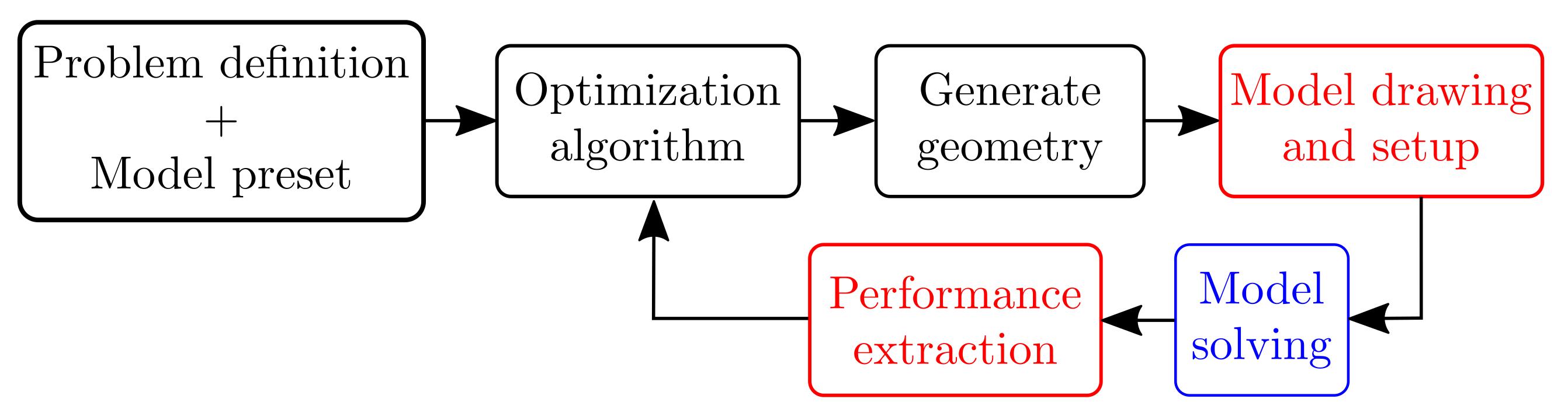
The applied optimization workflow is shown in Figure 5. The optimization process starts with the problem definition (boundaries, constraints, objectives, etc.) and a preset of constant parameters (slots, poles, active diameter, etc.).

After entering the optimization loop, the following steps are performed iteratively:

• the optimization algorithm generates the vector $\overrightarrow{x}$ (optimization variables);
• variables are converted to model parameters;
• model is generated based on the model parameters;
• model is solved;
• performance is extracted from the solution (values for constraints and objective functions are calculated from the solution);
• data is passed to the optimization algorithm.

Single-objective optimization has only one objective function, which may have multiple variables and scaling factors. When the optimization converges, the value of the objective function saturates around a certain value. Without stopping criteria, the objective function will improve in infinitesimal steps for a very long time without any significant design improvement. In this paper, the following stopping criteria are used: after each generation, the last four objective function increments $f_{1..4}$ are checked; if the difference between $f_1$ and $f_4$ is less than 0.2%, the optimization is stopped; otherwise, it continues until the 160th generation.

5. Model and Solution Feasibility

In optimization problems, the notion of feasibility is related to the acceptance criteria of the solution. A solution is declared feasible if it satisfies certain criteria (15). The feasibility of a solution implies that a solution exists, i.e., the problem or model that provides this solution is solvable. During the optimization process, models may occur that are not solvable. These models have no solution and can be declared infeasible without solving them, which can decrease computational burden in the case of FEA-based solver. The models that are not solvable are declared as infeasible considering the model feasibility criteria.

5.1. Geometrical Feasibility

A special subset of model feasibility criteria is geometric feasibility, which characterizes whether the model geometry satisfies certain criteria (e.g., mechanical integrity, physicality, overlaps, etc.). In some cases, trying to solve a geometrically infeasible model with external solvers can lead to a crash of the whole optimization routine, a problem that highlights the need for detection methods to deal with geometrically infeasible models (e.g., barrier 1 (blue) collides with barrier 2 (yellow), the overlap is marked in red, Figure 6c).

To avoid the construction of such an invalid model, a geometric feasibility procedure can be performed within the optimization algorithm for each candidate vector. Regardless of the method of handling and detecting geometric infeasibility, it is always beneficial to reduce the occurrence of infeasible models. The simplest method for reducing the occurrence of geometrically infeasible models is to introduce lower and upper parameter bounds, which can be in the form of linear (Figure 7a), non-linear function bounds (Figure 7b), or complex bounds (Figure 7c).

For simple problems, the introduction of bounds can completely avoid the occurrence of infeasible models, while for complex problems it reduces the probability of the occurrence of the infeasible candidates. For this reason, optimization algorithms must include a method for dealing with geometrically infeasible candidates.

In general, a geometrically infeasible candidate is discarded while the new candidate takes its place. To generate a replacement candidate, Žarko et al. [25,32] randomly initialize the entire parameter set (13) until a geometrically feasible replacement candidate appears. The drawback of this method is a possible rejection of candidates with some good properties. Moreover, this method may lead to slow convergence to the optimal solution if the optimal candidate is on the boundary of the feasible space.

The alternative approach is forced feasibility, where each infeasible design is subjected to parameter modification until feasibility is achieved (i.e., barrier 1 (blue) and barrier 2 (yellow) are modified until the candidate achieves the specified flux carrier width $w_{\mathrm{goal}}$, Figure 6d). This approach requires smart parametrization with minimum feasibility constraints and can potentially be extremely complex. On the other hand, potential benefits include reduced optimization time (no need to wait for a random feasible design to emerge) and faster convergence to the final result. The substitution of infeasible candidates is implemented in the form of a projection onto the feasible space (Figure 7d).

Projection operator can be mathematically written as:

$$\begin{array}{cc}\hfill P& =min[({\overrightarrow{x}}_{\mathrm{orig}}-{\overrightarrow{x}}_{\mathrm{new}})·Q{({\overrightarrow{x}}_{\mathrm{orig}}-{\overrightarrow{x}}_{\mathrm{new}})}^T],\hfill \end{array}$$

(17)

$$\begin{array}{cc}\hfill Q& =\left[\begin{array}{cccc}{q}_1& 0& \cdots & 0\\ 0& q_2& \cdots & 0\\ ⋮& ⋮& \ddots & ⋮\\ 0& 0& \cdots & q_D\end{array}\right],\hfill \\ \hfill \forall {\overrightarrow{x}}_{\mathrm{new}}& \in R^D\hfill \end{array}$$

(18)

where ${\overrightarrow{x}}_{\mathrm{orig}}$ represents parameter vector of original, geometrically infeasible candidate, ${\overrightarrow{x}}_{\mathrm{new}}$ is its geometrically feasible replacement/alternative, and Q is weighting matrix (18) in which its coefficients control the projection path (1, 2, and 3 in Figure 7d). If all coefficients satisfy $q_{1..D}=1$, projection is orthogonal, and the new geometrically feasible candidate is closest to the original infeasible candidate.

5.2. Forced Feasibility Algorithm

For simplicity, the functionality is explained using two barrier SyRM (Figure 6b–d). The first step is geometry generation based on the parameterization approach from Section 3 (Algorithm 1: ln: 1–5). The next step is to compute the variables $d_{k-1,k},w_{k-1,k},w_{\mathrm{goal}}$ (Figure 6b) and check whether the infeasibility condition is satisfied (Algorithm 1: ln: 11). The design may be infeasible for one of two reasons: there is a barrier conflict ($w_{k-1,k}\le 0$) or the flux carrier width is too small ($w_{k-1,k}\le w_{\mathrm{goal}}$). If not feasible (Figure 6c), proceed to forcing feasibility (Algorithm 2).

The purpose of the force feasibility function (Algorithm 2: ln: 1) is to provide the current position information of the barrier ($w_{\mathrm{goal}},d_{k-1,k},\Delta r_{k_{out}},\Delta r_{k-1_{in}}$, Figure 6b) and provide minimally modified barrier offsets ($\Delta r_{k_{out}}^{\prime },\Delta r_{k-1_{in}}^{\prime }$), defining a new feasible design (Figure 6d). The minimal deviation is secured via MATLAB function FMinCon function [33]. FMinCon default input parameters are listed in Algorithm 2: ln: 2–7, where $x_c$ represents the current barrier offset vector.

During the search, FMinCon iteratively calls CostFcn, which is responsible for the convergence of the search (calculates the deviation of the generated x and the initial offset vector $x_c$), and ConstraintFcn which calculates the deviation of the generated flux carrier width (w) from the carrier width ($w_{\mathrm{goal}}$). When the algorithm converges, FMinCon returns $\Delta r_{k_{out}}^{\prime },\Delta r_{k-1_{in}}^{\prime }$, and a new feasible geometry is generated (Figure 6d).

In summary, when the system detects an infeasible case, such as in the example shown in Figure 6b, where 1st and 2nd barriers overlap, $\Delta r_{2\mathrm{out}}$ and $\Delta r_{1\mathrm{in}}$ are iteratively modified until flux carrier width $w_{\mathrm{goal}}$ is reached (Figure 6d). This prevents the generation of too thin or too wide barrier geometries and improves the optimization procedure. The flux carrier width is randomly generated according to the equation $w_{\mathrm{goal}}=d_{k-1,k}/R_{w_k}$ in the range $R_{w_k}=[1.561,1.88]$ (Figure 6a). The range is empirically derived from several optimized designs.

Algorithm 1 Check feasibility function
1: Get:
2: $r_{G_{1..k}}$	▹ Virtual barrier mid points
3: $\Delta r_{1..k_{out}}$	▹ Barrier outer offsets
4: $\Delta r_{1..k_{in}}$	▹ Barrier inner offsets
5: $R_{w_{1..k}}\to Rnd\left([1.561,1.88]\right)$	▹ Flux carrier width goal ratios
6: function CheckFeasibility
7:   for k=2:$N_{barriers}$ do
▹ Calculate distance between virtual barrier mid points
8:   $d_{k-1,k}=r_{G_{k-1}}-r_{G_k}$
▹Calculate flux carrier width
9:   $w_{k-1,k}=(r_{G_{k-1}}-\Delta r_{k-1_{in}})-(r_{G_k}+\Delta r_{k_{out}})$
▹ Calculate minimal flux carrier width
10:   $w_{\mathrm{goal}}=d_{k-1,k}/R_{w_k}$
11:   if $w_{k-1,k}\le 0$ or $w_{k-1,k}\le w_{\mathrm{goal}}$ then
▹ Barriers are not feasible, force feasibility
12:    function ForceFeasibility(
$w_{\mathrm{goal}},d_{k-1,k},\Delta r_{k_{out}}$, $\Delta r_{k-1_{in}}$)
13:     …
14:    return $\Delta r_{k_{out}}^{\prime },\Delta r_{k-1_{in}}^{\prime }$

Algorithm 2 Force feasibility function
1: function ForceFeasibility
2:  $A,B,A_{eq},B_{eq}=\left[\right]$	▹ empty FMinCon parametes
3:  $opt\to$ default	▹ Use default FMinCon options
4:  $lb=\left[00\right]$	▹ Lower minimization bounds
5:  $ub=\left[d_{k-1,k}{d}_{k-1,k}\right]$	▹ Uppper minimization bounds
6:  $x_0=0.5·ub$	▹ Initial guess
7:  $x_c=[\Delta r_{k_{out}}\Delta r_{k-1_{in}}]$	▹ Minimization goal
▹Find a solution which satisfies constraints and minimally changes input parameters $x_c$ via FMinCon function
8:  function FMinCon(CostFcn, $x_0,B,A_{eq},B_{eq},lb,ub$,ConstraintFcn, $w_{\mathrm{goal}},d_{k-1,k},x_c$, $opt$, k)
▹FMinCon iteratively calls CostFcn, ConstraintFcn and returns values which satisfy the constraint(s) with minimal deviation from current offset vector $x_c$
9:   …
10:  return $\Delta r_{k_{out}}^{\prime },\Delta r_{k-1_{in}}^{\prime }$
11:  function CostFcn($x,x_c,k$)
▹CosttFcn is responsible for result search convergence
12:   $f=(x-x_c){.}^2$
13:   $F=Sum\left(f\right)$
14:  return F
15:  function ConstraintFcn($x,w_{\mathrm{goal}},d_{k-1,k}$)
▹ConstraintFcn calculates the deviation of generated flux carrier width from the goal width
16:   $x\left(1\right)\to \Delta r_{k_{out}}$
17:   $x\left(2\right)\to \Delta r_{k-1_{in}}$
18:    $w=\left(r_{G_{k-1}}+x\left(2\right)\right)-\left(r_{G_k}+x\left(1\right)\right)$
19:    $=d_{k-1,k}-x\left(1\right)-x\left(2\right)$
20:   $P=w_{\mathrm{goal}}-w$
21:  return P
22: return $\Delta r_{k_{out}}^{\prime },\Delta r_{k-1_{in}}^{\prime }$

Overall, this system does not discard randomly generated infeasible geometry, but modifies it until feasibility is achieved (hence the name “forced” feasibility). A similar procedure can be implemented for any problem that can be described by smooth analytic functions implemented as user-defined ConstraintFcn.

5.3. Handling of Inequality Constraints

Inequality constraints usually arise from various electromagnetic, thermal, mechanical, manufacturing, economic, or normative limits, such as maximum flux density in the stator tooth, maximum magnet temperature, maximum stress in the rotor bridge, minimum magnet dimensions, maximum active material cost, maximum noise, etc. [32].

The traditional approach to constraint handling uses penalty functions to penalize the solutions that violate the constraints. This principle is implemented in terms of weighted sums that modify each objective function. Despite the popularity of penalty functions, they have several drawbacks. The most important is the need for careful fine-tuning of the penalty factors responsible for efficiently approximating the feasible range. Moreover, this method may suffer from problems related to poor choice of weighting factors, which may affect convergence. In this paper, we use an improved constraint function algorithm developed by Žarko et al. [34].

Inequality constraints for this particular case are defined in

Table 5. List of inequality constraints.

No:	Constraint Description	Symbol	Limit
$g_1$	Stress yield factor at $1.2·n_{\max }$	${\mathrm{FOS}}_{\min }$	≥2
$g_2$	Magnetostatic torque at $n_b$	$T_{\mathrm{static}}$	≥600 Nm
$g_3$	Flux density in stator yoke	$B_{\mathrm{sy},\max }$	≤1.6 T
$g_4$	Flux density in stator tooth	$B_{\mathrm{st},\max }$	≤1.8 T
$g_5$	Power factor	$cos{\phi }_{\min }$	>0.6
$g_6$	Torque ripple with skewing	$T_{\mathrm{ripple},\max }$	≤10 %

. The constraint function $g_1$ checks rotor structural factor of safety at maximum over-speed ($1.2·n_{\max }$).

The procedure related to constraint function $g_2$ contains several subfunctions designed according to ultra-fast scaling laws [29]. Multiple magnetostatic FEA calculations are performed to find the maximum torque versus current phase advance curve and to determine the optimal maximum torque-per-ampere (MTPA) control angle by polynomial fitting (the input machine has one turn per coil and one parallel path). The number of turns per coil and the number parallel paths of the machine is then matched to the required base speed. The optimization initially assumes a fixed stack length (Table 2, parameter $l_{\mathrm{s}\max }$). If the calculated torque at $l_{\mathrm{s}\max }$ is smaller than required, the machine design does not satisfy the constraint. Finally, it is checked whether the stator phase current is smaller than the maximum inverter current; otherwise, the constraint is not satisfied. After this step, all magnetostatic calculations are completed. The results are extracted and evaluated in the following constraint functions. Constraint $g_3$ checks the maximum stator yoke flux density, while $g_4$ checks the maximum tooth flux density. The purpose is to penalize the high saturation and the designs with increased iron losses.

Finally, a transient FEA calculation is performed at base speed to determine the power factor, average torque, torque ripple, and terminal voltage. Constraint $g_5$ checks the power factor. The primary goal in this ePTO optimization case study was maximization of the average torque, while torque ripple was of secondary importance, therefore being handled in the constraint ($g_6$). As a torque-ripple mitigation option, a rotor skew was selected. Skewing angle is one stator slot or ${360}^{\circ }/36={10}^{\circ }$ mechanical degrees [35]. Without loss of generality, other more affordable, or more practical, torque-ripple mitigation techniques can be applied to this problem [36,37]. In addition, torque ripple can be included as another optimization objective so that the design trade-off is made on the Pareto front of torque versus torque ripple.

If all constraints are satisfied, the final step is to compute the objective function f (19). $\eta$ is the efficiency, and $T_{\mathrm{trans},\mathrm{skew}}$ is the transient torque with applied rotor skew. The constants 700 and $0.96$ represent scaling coefficients, which are used for combining torque and efficiency within a single objective function. Furthermore, these values are important for proper optimization convergence and were intentionally chosen to be larger than the peak torque and efficiency at the base speed to constrain the objective function to values $\le 2$ (important for the final comparison of the optimization convergence of forced feasibility and randomly generated geometries).

$$\begin{array}{c}\hfill f=\frac{T_{\mathrm{trans},\mathrm{skew}}}{700}+\frac{\eta }{0.96}.\end{array}$$

(19)

6. Optimization Results

Five consecutive optimization runs of the DE algorithm with population size $\mathrm{NP}=24$ of geometries generated both randomly and with forced feasibility were performed (results in Table 4 and

Table 6. Optimization results.

Random Generated			Forced Feasibility
Generation	$\mathit{f}$	t [h]	Generation	$\mathit{f}$	t [h]
89	1.8129	20.3	77	1.8136	18.9
91	1.8124	21.2	87	1.8145	21.2
106	1.8128	24.9	88	1.8132	21.9
132	1.8128	31.5	94	1.8133	23.8
160	1.8124	37.5	132	1.8133	32.9
Average			Average
115.6	1.81266	27.08	95.6	1.81358	23.74

).

To reduce optimization time and compare both approaches, most of the design parameters were taken from a previously optimized design [3]. Twenty-eight parameters were frozen (Table 2), and only 7 parameters were used for optimization (Table 3). This trade-off yields the same average objective function result (difference is +0.05%).

The average number of generations required to achieve convergence in the random generation case is 115.6, and 95.6 in the forced feasibility case, which is a reduction of 17.3%. In addition, in terms of computation time, the average convergence of forced feasibility is 3.34 h shorter (12.3% reduction).

When comparing the average torque results ($T_{\mathrm{trans},\mathrm{skew}}$), both approaches yield practically the same outcome (Table 4). The remaining results ($\eta ,B_{\mathrm{sy},\max },B_{\mathrm{st},\max },cos\phi ,T_{\mathrm{ripple}}$) are identical for forced feasibility and random generation. This is expected for two reasons: most of the parameters were taken from Reference [3], and the optimization algorithm is the same. Finally, the identical results confirm that forced feasibility does not affect negatively the optimization outcome.

Table 4 summarizes the optimized rotor parameters for both optimization approaches. As mentioned earlier, the most important result is the fact that all parameters are greater than zero (neither the inner nor the outer blocking line sticks to the virtual centerline) and $\forall \Delta r_{k_{\mathrm{out}}}\ne \forall \Delta r_{k_{\mathrm{in}}}$. All optimized cross sections are shown in Figure 8, which confirms that the position of the centerline of the virtual barriers does not affect the optimization result.

7. Conclusions

This paper demonstrates a novel automatic design procedure of SyRM rotor with minimum number of geometric parameters, which simplifies the design generation and reduces the optimization time. The presented procedure is implemented into an existing single objective DE optimization algorithm framework which interrupts evaluation of constraint functions when the inequality constraint is violated, thus saving computation time.

The second paper contribution is the introduction of novel forced feasibility concept which improves optimization convergence proved by successive comparative optimization runs with randomly generated rotor barrier geometries. The results show that properly implemented forced feasibility leads to a further reduction in optimization time (12.3% shorter).

The machine design originally presented in Reference [3] has 21 optimization variables. The entire optimization process took 7 days. Without the forced feasibility method, the process would be 12.3% longer (approximately 1 additional day). Considering that the optimization time is proportional to the number of parameters (i.e., a two- layer V-shape PM machine may have 44 parameters), it can be concluded that the total calculation time can be significantly reduced by using forced feasibility approach on different machine topologies.

References

- European Environment Agency. Electric Vehicles in Europe. Available online: https://www.eea.europa.eu/publications/electric-vehicles-in-europe (accessed on 2 January 2012).
- Ban, B.; Stipetić, S. Electric Multipurpose Vehicle Power Take-Off: Overview, Load Cycles and Actuation via Synchronous Reluctance Machine. In Proceedings of the 2019 International Aegean Conference on Electrical Machines and Power Electronics (ACEMP) & 2019 International Conference on Optimization of Electrical and Electronic Equipment (OPTIM), Istanbul, Turkey, 27–29 August 2019. [Google Scholar]
- Ban, B.; Stipetic, S. Design and Optimization of Synchronous Reluctance Machine for actuation of Electric Multi-purpose Vehicle Power Take-Off. In Proceedings of the 2020 International Conference on Electrical Machines (ICEM 2020), Gothenburg, Sweden, 23–26 August 2020; p. 1. [Google Scholar]
- Alberti, L.; Bianchi, N.; Boglietti, A.; Cavagnino, A. Core axial lengthening as effective solution to improve the induction motor efficiency classes. In Proceedings of the IEEE Energy Conversion Congress and Exposition: Energy Conversion Innovation for a Clean Energy Future (ECCE 2011), Phoenix, AZ, USA, 17–22 September 2011. [Google Scholar]
- Bramerdorfer, G.; Cavagnino, A.; Vaschetto, S. Impact of IM pole count on material cost increase for achieving mandatory efficiency requirements. In Proceedings of the IECON (Industrial Electronics Conference), Florence, Italy, 24–27 October 2016. [Google Scholar]
- Agamloh, E.B.; Boglietti, A.; Cavagnino, A. The incremental design efficiency improvement of commercially manufactured induction motors. IEEE Trans. Ind. Appl. 2013, 49, 2496–2504. [Google Scholar] [CrossRef]
- El-Refaie, A.M. Motors/generators for traction/propulsion applications: A review. IEEE Veh. Technol. Mag. 2013, 8, 90–99. [Google Scholar] [CrossRef]
- Pellegrino, G.; Cupertino, F.; Gerada, C. Automatic Design of Synchronous Reluctance Motors Focusing on Barrier Shape Optimization. IEEE Trans. Ind. Appl. 2015, 51, 1465–1474. [Google Scholar] [CrossRef]
- Lu, C.; Ferrari, S.; Pellegrino, G. Two Design Procedures for PM Synchronous Machines for Electric Powertrains. IEEE Trans. Transp. Electrif. 2017, 3, 98–107. [Google Scholar] [CrossRef]
- Zhu, X.; Wu, W.; Quan, L.; Xiang, Z.; Gu, W. Design and Multi-Objective Stratified Optimization of a Less-rare-earth Hybrid Permanent Magnets Motor with High Torque Density and Low Cost. IEEE Trans. Energy Convers. 2018, 34, 1178–1189. [Google Scholar] [CrossRef]
- Bonthu, S.S.R.; Choi, S.; Baek, J. Design Optimization with Multiphysics Analysis on External Rotor Permanent Magnet-Assisted Synchronous Reluctance Motors. IEEE Trans. Energy Convers. 2018, 33, 290–298. [Google Scholar] [CrossRef]
- Tapia, J.A.; Parviainen, A.; Pyrhonen, J.; Lindh, P.; Wallace, R.R. Optimal design procedure for an external rotor permanent-magnet machine. In Proceedings of the 2012 20th International Conference on Electrical Machines (ICEM 2012), Marseille, France, 2–5 September 2012. [Google Scholar]
- Lei, G.; Bramerdofer, G.; Ma, B.; Guo, Y.; Zhu, J. Robust Design Optimization of Electrical Machines: Multi-objective Approach. IEEE Trans. Energy Convers. 2020, 36, 390–401. [Google Scholar] [CrossRef]
- Lei, G.; Bramerdorfer, G.; Liu, C.; Guo, Y.; Zhu, J. Robust Design Optimization of Electrical Machines: A Comparative Study and Space Reduction Strategy. IEEE Trans. Energy Convers. 2020, 36, 300–313. [Google Scholar] [CrossRef]
- Babetto, C.; Bacco, G.; Bianchi, N. Synchronous Reluctance Machine Optimization for High-Speed Applications. IEEE Trans. Energy Convers. 2018, 33, 1266–1273. [Google Scholar] [CrossRef]
- Xu, L.; Wu, W.; Zhao, W.; Liu, G.; Niu, S. Robust Design and Optimization for a Permanent Magnet Vernier Machine With Hybrid Stator. IEEE Trans. Energy Convers. 2020, 35, 2086–2094. [Google Scholar] [CrossRef]
- Howard, E.; Kamper, M.J. Weighted Factor Multiobjective Design Optimization of a Reluctance Synchronous Machine. IEEE Trans. Ind. Appl. 2016, 52, 2269–2279. [Google Scholar] [CrossRef]
- Kamper, M.J.; Van Der Merwe, F.S.; Williamson, S. Direct Finite Element Design Optimisation of the Cageless Reluctance Synchronous Machine. IEEE Trans. Energy Convers. 1996, 11, 547–553. [Google Scholar] [CrossRef]
- Dmitrievskii, V.; Prakht, V.; Kazakbaev, V. IE5 Energy-Efficiency Class Synchronous Reluctance Motor with Fractional Slot Winding. IEEE Trans. Ind. Appl. 2019, 55, 4676–4684. [Google Scholar] [CrossRef]
- Yamashita, Y.; Okamoto, Y. Design Optimization of Synchronous Reluctance Motor for Reducing Iron Loss and Improving Torque Characteristics Using Topology Optimization Based on the Level-Set Method. IEEE Trans. Magn. 2020, 56, 36–39. [Google Scholar] [CrossRef]
- Storn, R.; Price, K. Differential Evolution—A Simple and Efficient Heuristic for Global Optimization over Continuous Spaces. J. Glob. Optim. 1997, 11, 341–359. [Google Scholar] [CrossRef]
- Bramerdorfer, G.; Zavoianu, A.C.; Silber, S.; Lughofer, E.; Amrhein, W. Possibilities for Speeding Up the FE-Based Optimization of Electrical Machines-A Case Study. IEEE Trans. Ind. Appl. 2016, 52, 4668–4677. [Google Scholar] [CrossRef]
- Liu, X.; Slemon, G.R. An improved method of optimization for electrical machines. IEEE Trans. Energy Convers. 1991, 6, 492–496. [Google Scholar] [CrossRef]
- Stipetic, S.; Zarko, D.; Kovacic, M. Optimised design of permanent magnet assisted synchronous reluctance motor series using combined analytical-finite element analysis based approach. IET Electr. Power Appl. 2016, 10, 330–338. [Google Scholar] [CrossRef]
- Zarko, D.; Stipetic, S.; Martinovic, M.; Kovacic, M.; Jercic, T.; Hanic, Z. Reduction of computational efforts in finite element-based permanent magnet traction motor optimization. IEEE Trans. Ind. Electron. 2017, 65, 1799–1807. [Google Scholar] [CrossRef]
- Lampinen, J. Multi-Constrained Nonlinear Optimization by the Differential Evolution Algorithm. In Soft Computing and Industry; Springer: London, UK, 2002. [Google Scholar]
- Price, K.; Storn, R. Matlab Code for Differential Evolution. Available online: http://www1.icsi.berkeley.edu/$\sim$storn/code.html (accessed on 23 January 2020).
- Motor Design Ltd. Motor-CAD/Motor-LAB Software. Available online: https://www.motor-design.com/motor-cad/ (accessed on 23 January 2020).
- Stipetic, S.; Zarko, D.; Popescu, M. Ultra-fast axial and radial scaling of synchronous permanent magnet machines. IET Electr. Power Appl. 2016, 10, 658–666. [Google Scholar] [CrossRef]
- Gamba, M.; Pellegrino, G.; Cupertino, F. Optimal Number of Rotor Parameters for the Automatic Design of Synchronous Reluctance Machines. In Proceedings of the 2014 International Conference on Electrical Machines (ICEM 2014), Berlin, Germany, 2–5 September 2014; pp. 1334–1340. [Google Scholar]
- Cupertino, F.; Pellegrino, G.; Cagnetta, P.; Ferrari, S.; Perta, M. SyRE: Synchronous Reluctance (Machines)—Evolution. Available online: https://sourceforge.net/projects/syr-e/ (accessed on 23 April 2021).
- Stipetic, S.; Miebach, W.; Zarko, D. Optimization in design of electric machines: Methodology and workflow. In Proceedings of the Joint International Conference—ACEMP 2015: Aegean Conference on Electrical Machines and Power Electronics, OPTIM 2015: Optimization of Electrical and Electronic Equipment and ELECTROMOTION 2015: International Symposium on Advanced Electromechanical Moti, Side, Turkey, 2–4 September 2015; pp. 441–448. [Google Scholar]
- Mathworks. Matlab Fmincon Function. Available online: https://se.mathworks.com/help/optim/ug/fmincon.html (accessed on 13 January 2020).
- Žarko, D.; Stipetić, S. Criteria for optimal design of interior permanent magnet motor series. In Proceedings of the 2012 20th International Conference on Electrical Machines (ICEM 2012), Marseille, France, 2–5 September 2012. [Google Scholar]
- Bomela, X.B.; Kamper, M.J. Effect of Stator Chording and Rotor Skewing on Performance of Reluctance Synchronous Machine. IEEE Trans. Ind. Appl. 2002, 38, 91–100. [Google Scholar] [CrossRef]
- Ferrari, S.; Armando, E.; Pellegrino, G. Torque Ripple Minimization of PM-assisted Synchronous Reluctance Machines via Asymmetric Rotor Poles. In Proceedings of the 2019 IEEE Energy Conversion Congress and Exposition (ECCE), Baltimore, MD, USA, 29 September–3 October 2019; pp. 4895–4902. [Google Scholar]
- Ferrari, S.; Pellegrino, G.; Davoli, M.; Bianchini, C. Reduction of Torque Ripple in Synchronous Reluctance Machines through Flux Barrier Shift. In Proceedings of the 2018 XIII International Conference on Electrical Machines (ICEM), Alexandroupoli, Greece, 3–6 September 2018; pp. 2290–2296. [Google Scholar]