BIBC Matrix Modification for Network Topology Changes: Reconfiguration Problem Implementation

Abstract

The topology of a distribution network can be represented by a bus injection to branch current (BIBC) matrix. It has been introduced and used for load flow analysis of distribution networks. In this paper, a method for BIBC matrix modification is developed to use in applications which require a topology change representation. Proposed method that reflects the changes in configuration in the system BIBC matrix is implemented in distribution network reconfiguration problem. With providing potential solutions for network operational and planning requirements such as necessitate changes in configurations to transfer the loads to a different substation, ease the loading of equipment, conduct planned maintenance and reduce network losses during the normal operation with renewables, storage and other uprising technologies, reconfiguration may also be useful for emergencies, accidents, attacks and weather-related disasters. The BIBC modification process provides the knowledge of possible switches to open and the direction of power flow without any need to further radiality or continuity check. The proposed method needs only initial network topology information that makes it suitable to apply on any distribution network and to use with any search method or heuristic/meta-heuristic optimization algorithm. Efficiency of the method is investigated on systems with voltage dependent and time varying loads.

1. Introduction

In power network, distribution networks play an important role as it is the final part to supply consumers. Due to its radial structure, unbalanced distributed loads with a great number of branches and nodes may cause challenges in network planning, state estimation, distributed energy sources integration, switching operations and load flow analysis. Linear methods for distribution network analysis have an important role both in planning and operation to deal with these challenges [1]. Linear approaches are widely used in power flow analysis [2,3,4], power loss estimation with distributed generation [5,6], and power network optimization studies [7].

One of the direct approaches [2] that only use the conventional bus–branch-oriented data, has been widely implemented for load flow calculations of distribution networks [8,9,10,11]. Bus injection to branch current matrix is introduced for the first time with this approach to develop a formulation for load flow analysis of the distribution network [2]. To solve distribution load flow directly, two relationship matrices are developed based on topological structure of distribution system: branch current to bus voltages (BCBV) and bus current injections to branch currents (BIBC). These two matrices are used to form a direct approach for load flow instead of time-consuming iterative methods which use the Jacobian matrix or Y admittance matrix [12,13,14]. Later, considering from a different angle BIBC is used for deriving a power loss formulation [6] to develop an analytical method for distributed generation placement problem. Branch currents are expressed by bus current injections to form the BIBC matrix and this provides the direct calculation of branch currents corresponding to the variation in bus current injections which is used to obtain power loss. This analytical formula leads a discussion about power loss estimation of a network after any topology change. Reflecting the network topology change in BIBC matrix can be useful to implement network operational requirements such as necessitate changes in configurations to transfer the loads to a different substation, ease the loading of equipment, and conduct planned maintenance, etc. These operations are called as reconfiguration which is simply changing the topology of distribution network by opening or closing pre-installed switches, while keeping the radial structure of feeders. Those sectionalizing switches are widely used in primary distribution systems to increase service reliability [15]. Network reconfiguration can be used to reduce power losses to relieve overloads or to provide power to all customers in a fault or outage [16]. Reconfiguration is one of the most discussed problems in power system optimization in last forty years and generally methods have been implemented to use reconfiguration as a loss minimization technique. As well as being used as a tool for planning and operation in normal state of networks with renewables, storage and other uprising technologies, reconfiguration may also be useful for emergencies, accidents, attacks, and weather-related disasters. Such disturbances may cause damage in distribution network and repairs required to restore energy may take hours [17]. Changing topology may increase network resiliency by providing the ability to tolerate, adapt and recover from disasters [18]. Although a basic control action -a switching operation- involves in reconfiguration, discrete nature of switches, many switching combinations and radiality constraint transform the optimization problem into a mixed integer form. Hence majority of the methods for solving this problem are based on heuristic techniques.

The essential challenges of reconfiguration problem are to decide a switching procedure that ensures all loads are supplied and network remains radial as well as a need for fast loss estimation with simple calculations. The switching operation in reconfiguration have two types: branch exchange and loop cutting. The branch exchange method works in a radial system by opening and closing switch pairs, loop cutting opens switches in an initially meshed system until it becomes radial [19]. In early studies loop cutting is used for line loss minimization with a heuristic approach [20] while other use branch exchange method for the same objective. A simple formula with assumptions was derived by Civanlar et al. [21] for change in loss reduction to eliminate switching options. Baran and Wu [16] follow the same approach of Civanlar and use reconfiguration for loss minimization and load balancing with a heuristic method. However, their spanning tree method does not ensure global optimal solution since algorithm depends on initial branch selection and does not examine all possible trees. Goswami and Basu [22] presented a heuristic algorithm based on optimal flow pattern which is determined by solving Kirchhoff’s Voltage Law (KVL) and Kirchhoff’s Current Law (KCL) equations of network. Nature inspired metaheuristic algorithms are also used for solving reconfiguration problems. These are genetic algorithm (GA) [23], ant colony search algorithm (ACO) [24], harmony search algorithm (HSA) [25], particle swarm optimization algorithm (PSO) [26], bacterial foraging optimization algorithm (BFOA) [27], fireworks algorithm (FWA) [28], improved cuckoo search algorithm (ICSA) [29], selective firefly algorithm [30], adaptive shuffles frogs leaping algorithm (ASFLA) [31], hybrid grey wolf and particle swarm algorithm (GWO-PSO) [32], stochastic fractal search algorithm (SFS) [33] which have complex parameter selection and tuning despite some of them require less computation time.

Generally, in reconfiguration studies an optimal configuration is determined for a specific time point, but for realistic systems with time varying loads optimal time intervals and different reconfigurations may be considered within a specific time period. Variation of load during the time period is usually evaluated using different load types with different characteristics, like residential, commercial and industrial [34]. Optimization for such systems generally solved with heuristic methods that focus on operation expenses minimization considering switching loss and deteriorations of switches’ lifespan [35]. Problems are also modelled as multi-objective considering placement of renewables [36,37,38], electric vehicles [39], load balancing [40], maximum voltage deviation, etc. A number of reconfiguration studies used BIBC matrix for load flow calculations [28,41].

In reconfiguration problem, besides its large combinatorial solution space and discrete nature of switches, changing switch status on/off with certain constraints such as radiality and continuity and representing the changed topology for further analysis are the main challenges. Most of the studies first randomly change the switch status on or off and check if the new network ensures the radial structure and continuity then, reorder the network data for power flow calculations and loss estimation. Therefore, infeasible switching operations are created and then eliminated with further controls that causes computational burden. Moreover, power loss calculations with load flow analysis are time-consuming.

Introduction of BIBC matrix for power flow analysis [2] and presentation of an analytical formula for power loss estimation using BIBC matrix [6] constituted the motivation of this paper. A method is introduced for BIBC matrix modification to reflect the network topology changes. Proposed method removes the necessity of controlling both radiality and continuity constraints. The method provides branch numbers in the formed loop after closing a switch which are the candidate switches to open and shows changed current flow directions. Thus, the system remains radial, all loads are supplied without any further checks, and power loss of new configuration is obtained using the analytical formula [6] instead of power flow analysis.

Proposed modification method is implemented in a grid search algorithm which ensures the exact solution to reconfiguration problem by trying all switching combinations. The algorithm is performed both with the analytical power loss formula and power loss estimation with power flow analysis. The analytical power loss calculation assumes system loads as constant current which might be convenient for distribution networks rather than the conventional constant power approach. Due to non-identical results for examined systems with 33 and 69 bus in literature, the exact solution is also calculated with power flow analysis using voltage dependent load models to investigate effects of different loads and compare results with an analytical loss formula. In terms of calculation time, grid search may fall behind the heuristic or metaheuristic approaches, in this study it is chosen to reach the exact solution without any concerns, like local optima or parameter tuning, and shows the effectiveness of using proposed BIBC modification method and the analytical power loss calculation together in terms of time and calculation simplicity.

The rest of the paper is organized as follows: The formulation of power loss is given in Section 2, BIBC modification is explained in detail in Section 3, a grid search algorithm is presented in Section 4, load models used in the paper given in Section 5, Section 6 develops the reconfiguration analysis, results are discussed in Section 7 and conclusion is given in Section 8.

2. Analytical Power Loss Calculation for Distribution Networks

Total power loss of a system can be calculated using branch currents and line resistances. Branch current and bus current injection relationship is obtained by applying KCL. Loads are assumed as constant currents. Branch currents vector $B$ is obtained with bus current injections vector $I$ and bus injection to branch current matrix $\mathrm{BIBC}$ as in (1) [2].

$${\left[B\right]}_{nb}={\left[\mathrm{BIBC}\right]}_{nbx(n-1)}{\left[I\right]}_{(n-1)x1}$$

(1)

Here, $n$ is the number of buses, $nb$ is the number of branches, $I$ is the bus current injection vector excluding swing bus. Total power loss can be written by using resistances $R$ and branch currents $B$ as follows [6]:

$$P_{loss}={\displaystyle \sum }_{i=1}^{nb}{\left|B_i\right|}^2{R}_i={\left[R\right]}^T{\left|\left[\mathrm{BIBC}\right]\left[I\right]\right|}^2$$

(2)

To use (2) in reconfiguration, changes on system topology should be represented in the equation. Although bus current injections remain constant for the new configuration, BIBC matrix which represents the branch currents is changed. Resistance vector also needs to be revised for the lines removed and added. The changes are shown in (3) with revised resistance vector as $rR$ and reconfigured BIBC matrix as $r\mathrm{BIBC}$.

$$P_{los{s}_r}={\left[rR\right]}^T{\left|\left[r\mathrm{BIBC}\right]\left[I\right]\right|}^2$$

(3)

$P_{los{s}_r}$ provides the power loss of reconfigured network and $rR$ is achieved with exchanging the line resistance of removed branch with the added one. Modifying $\mathrm{BIBC}$ matrix and building $r\mathrm{BIBC}$ matrix will be detailed in Section 3.

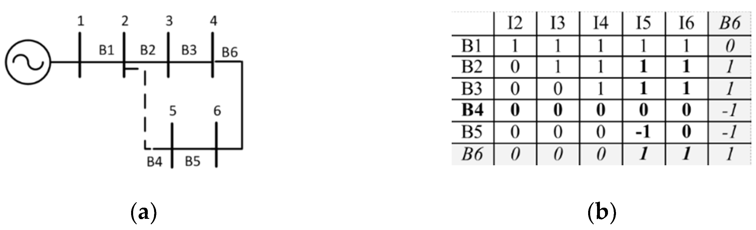
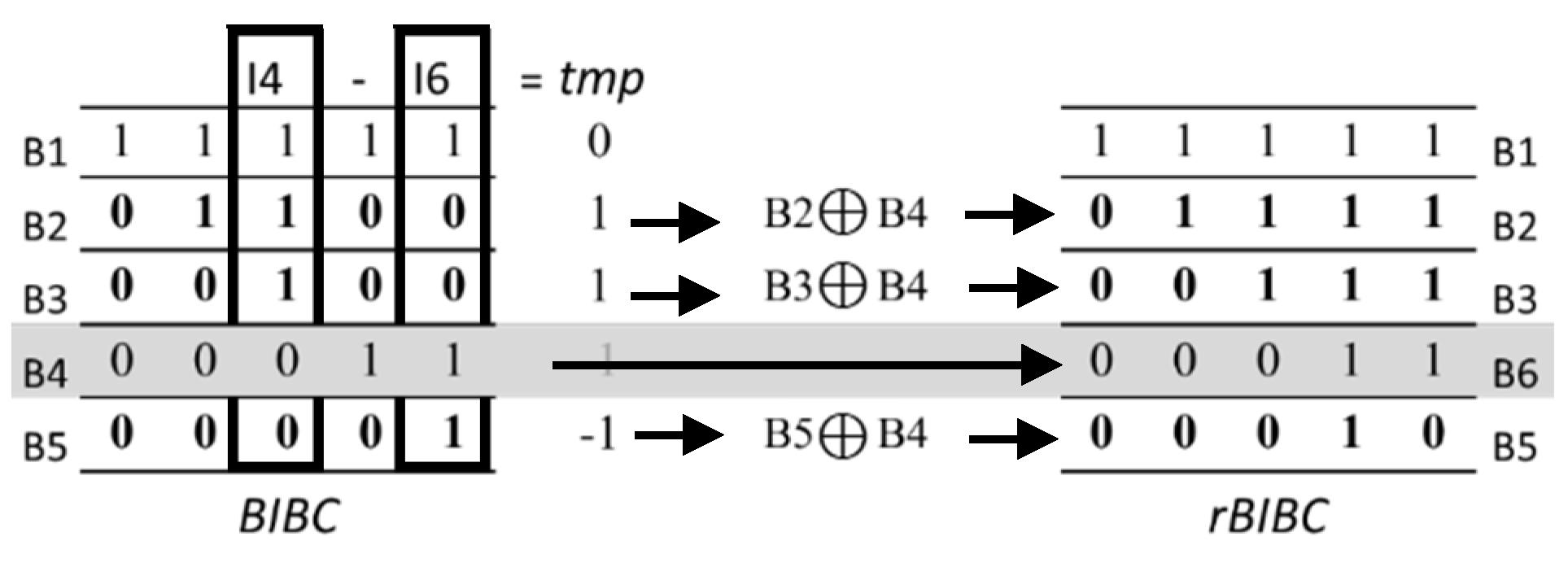
3. BIBC Matrix Modification for Topology Change Representation

To change topology of a distribution network, a tie switch is closed, a loop is formed, and a sectionalizing switch is opened to satisfy radiality. Bus current injections do not change when a loop formed, but new branch need to be added to network. Similarly, existing branch will need to be removed when a switch is opened. As bus injections do not change, BIBC matrix will need to be modified to calculate power loss with (3) for the new network configuration.

A six-bus system in Figure 1a is used to explain BIBC modification process. Branch currents of the six-bus system is given in (4).

$$\left[B\right]=\left[\mathrm{BIBC}\right]\left[I\right]$$

$$\left[\begin{array}{c}{B}_1\\ B_2\\ B_3\\ B_4\\ B_5\end{array}\right]=\left[\begin{array}{c}\begin{array}{ccc}1& 1& 1\\ 0& 1& 1\\ 0& 0& 1\end{array} \begin{array}{cc}1& 1\\ 0& 0\\ 0& 0\end{array}\\ \begin{array}{ccc}0& 0& 0\end{array} \begin{array}{cc}1& 1\end{array}\\ \begin{array}{ccc}0& 0& 0\end{array} \begin{array}{cc}0& 1\end{array}\end{array}\right] \left[\begin{array}{c}{I}_2\\ I_3\\ I_4\\ I_5\\ I_6\end{array}\right]$$

(4)

Assume there is a tie switch between bus 4 and 6 as shown with dashed line in Figure 1a. BIBC matrix is given as a table in Figure 1b to explain further steps clearly.

Branch-6 (B6) is the branch to close, $B_{cl}$. A loop is formed as in Figure 2a. After adding B6, current injections of bus 4 and 6 will be like in (5). B6 is represented as on table in Figure 2b.

$$I_4^{\prime }=I_4+B_6 I_6^{\prime }=I_6-B_6$$

(5)

Nonzero rows of B6 column give the information of branches which formed a loop. The branch to open, $B_{op}$, should be selected from one of the branches B2, B3, B4, B5 or B6 itself to keep the system radial. Assuming Branch-4 is opened, B4 row should be equal to zero as in (6). In this case, B6 is equal to the sum of injection currents of buses 5 and 6 as in (7).

$$B_4=I_5+I_6-B_6=0$$

(6)

$$B_6=I_5+I_6$$

(7)

BIBC matrix is updated with using (7). Branches those formed a loop are affected with added line. Opened branch, B4, row of BIBC matrix become zero as in Figure 3b. Negative value on the B5 row indicates power flow direction is changed on 5th branch. Closed line B6 is replaced with opened one B4 on BIBC matrix and branch currents of reconfigured system as in Figure 3a are given in (8).

$$\left[rB\right]=\left[r\mathrm{BIBC}\right]\left[I\right]$$

$$\left[\begin{array}{c}{B}_1\\ B_2\\ B_3\\ B_6\\ B_5\end{array}\right]=\left[\begin{array}{c}\begin{array}{ccc}1& 1& 1\\ 0& 1& 1\\ 0& 0& 1\end{array} \begin{array}{cc}1& 1\\ 1& 1\\ 1& 1\end{array}\\ \begin{array}{ccc}0& 0& 0\end{array} \begin{array}{cc}1& 1\end{array}\\ \begin{array}{ccc}0& 0& 0\end{array} \begin{array}{cc}1& 0\end{array}\end{array}\right] \left[\begin{array}{c}{I}_2\\ I_3\\ I_4\\ I_5\\ I_6\end{array}\right]$$

(8)

Given procedure above can be implemented as follows: Branch to close, $B_{cl}$, between bus j and k, is selected. A temporary vector, $temp$, is obtained with subtracting $I_k$ column of BIBC from $I_j$ column $\left(\left[I_j\right]-\left[I_k\right]\right)$. To keep radiality, one of the branches of the loop should be opened ($B_{op}$). In BIBC matrix, an XOR operation is performed between $B_{op}$ row and the nonzero rows of $tmp$ that give the branches of the loop. Finally, in $r\mathrm{BIBC}$ matrix name of the opened branch is exchanged with closed one, $B_{cl}$.

For the system in Figure 1a, branch to close ($B_{cl}$), B6, is connected from bus 4 to bus 6 and $tmp$ vector is obtained as in Figure 4. B4 is selected as branch to open $B_{op}$ and XOR operation is done between B4 row and B2, B3, B5 which are nonzero rows of $tmp$ vector. Opened branch B4 is changed to closed branch B6, and the $r\mathrm{BIBC}$ matrix is obtained as in Figure 4.

Modification methodology of BIBC matrix can be implemented using pseudo code given below:

Algorithm

Determine branch to close $B_{cl}$ between bus $j$ and bus $k$. Build a temporary vector. Nonzero rows give the branch numbers of loop: $\hspace{1em}\hspace{1em}\hspace{1em}\hspace{1em}tmp=\left|\mathrm{BIBC}\left(:,j-1\right)-\mathrm{BIBC}\left(:,k-1\right)\right|$ Choose branch to open $B_{op}$ in the loop using $tmp$ vector. Make $tmp\left(op\right)=0$. Form $\left[r\mathrm{BIBC}\right]$ by performing XOR logical operation between open branch row $\mathrm{BIBC}\left(op,:\right)$ and each row of BIBC matrix where $tmp=1$. Exchange the open branch $B_{op}$ with closed branch $B_{cl}$ in the branch current vector $\left[B\right]$ to obtain new branch current vector $\left[rB\right]$ of the new configuration.

Modification steps of $\mathrm{BIBC}$ matrix for a pair of closed opened switches are used in searching all possible switching options systematically, which explained in detail with grid search algorithm in Section 4.

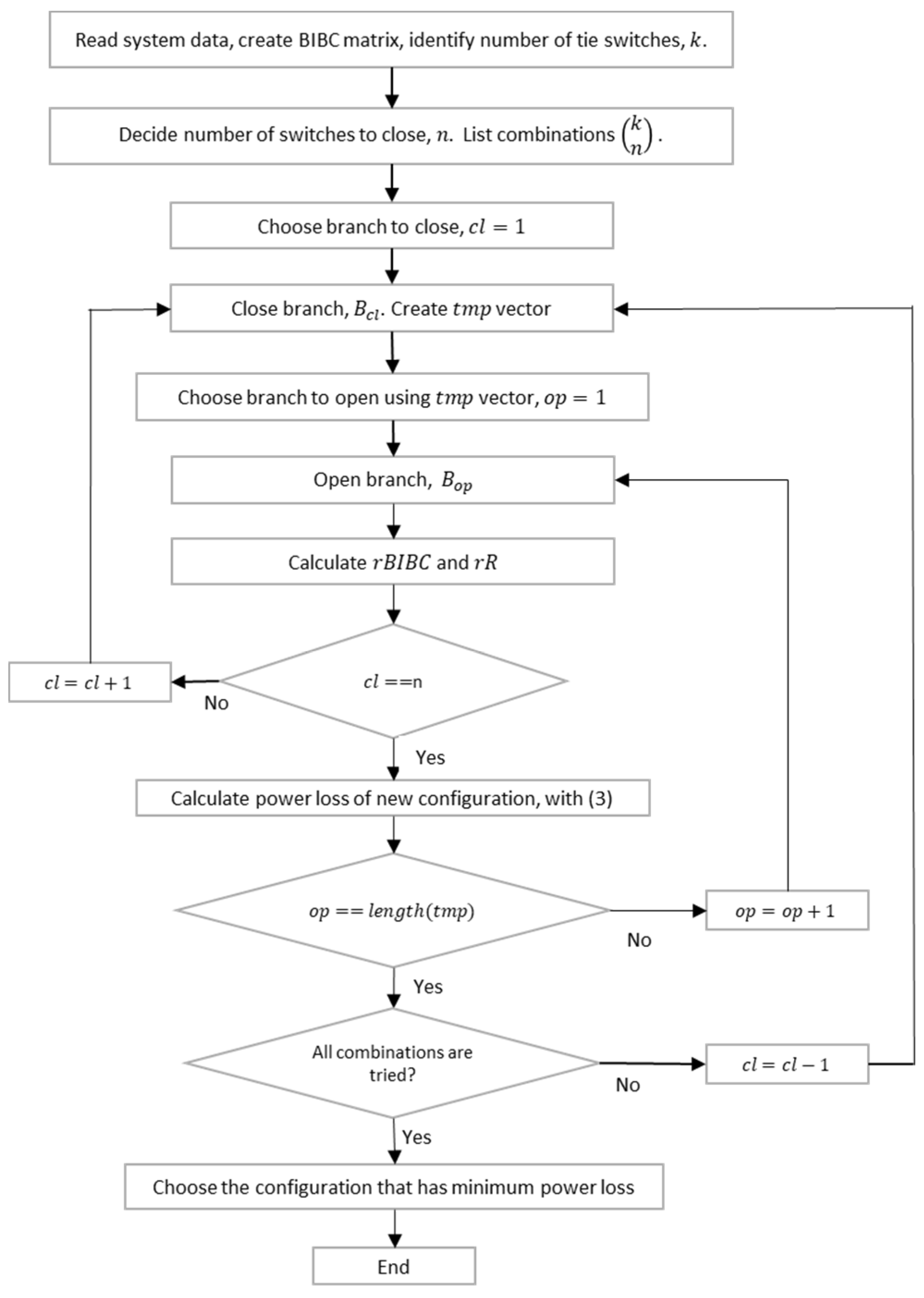
4. Problem Definition and Grid Search Algorithm for Reconfiguration

The use of reconfiguration to obtain minimum power loss can be obtained as in (9) where $P_{loss}$ is for the total loss of network and $B_i$ is the current of branch $i$ subject to voltage, current and radial topology constraints as in (10). Current of each branch $\left(B_i\right)$ must be under its permissible limit. Voltage magnitude $\left(V_i\right)$ at each node must be between pre-defined range.

$$\min P_{loss}={\displaystyle \sum }_{i=1}^{nb}{\left|B_i\right|}^2{R}_i$$

(9)

$$B_i<B_{max}$$

$$V_{min}<V_i<V_{max}$$

(10)

$$radial network structure$$

In reconfiguration studies, majority of search methods for the best network topology are based on heuristic algorithms as considerable number of switching and discrete nature of switch increase complexity of the problem.

However, grid search algorithm is the only method that allows examine of all possible switching combinations in a network thus ensures the exact solution. In grid search, tie switches number of the network, $k$, number of tie switches which are included in reconfiguration, n, are identified, all possible tie switch combinations are listed, and search process starts. Tie switch combinations are listed as vectors to enable choosing how many of those are used for reconfiguration. Once a tie switch is closed and the first candidate branch in the loop is opened, second tie switch is closed, and the first candidate branch of the new loop is opened, and this is repeated until the last tie switch. After the last tie switch is closed, all branches in the loop are opened one by one and power loss is calculated. Then algorithm starts to go back to the first loop step by step. At each step the whole topology of network changes due to new formed loops. Grid search is performed by a recursive function to ensure all combinations are examined. Proposed method, changing the network topology with BIBC modification, provides feasible switching combinations at each step through its capability of keeping system radial and operable without additional checking for radiality or continuity. Steps of algorithm is given as follows:

Algorithm

Read system data, create BIBC matrix, identify number of tie switches, $k$. Decide number of switches to close, $n.$ List combinations $\left(\begin{array}{c}k\\ n\end{array}\right)$.   Repeat for each combination vector. Choose branch to close $B_{cl} , cl=1..n$ Close branch $B_{cl}$, create $tmp$ vector. Open branch $B_{op}$, $op=1..lenght\left(tmp\right)$ Calculate $r\mathrm{BIBC}$ and $rR$ if    $cl\ne n$ do   $cl=cl+1$, turn 3   else if   $op \ne length\left(tmp\right)$    do  Calculate power loss for new configuration   $op=op+1$, turn 5    else   Calculate power loss for new configuration   $cl=cl-1$, turn 3   end Choose the configuration with minimum power loss as solution.

Flowchart of algorithm is given in Figure 5.

5. Distribution Network Load Modelling

Loads with different characteristics and types may be present in real distribution networks. As proposed method with analytical formula take network loads as constant current injections, conventional power flow studies in literature generally assume loads as constant power. To investigate effect of load characteristics in reconfiguration studies, in this paper static load modelling is considered, and analysis for distribution system with different load characteristics is performed. A backward-forward sweep method [42] for distribution systems power flow analysis is used to compare reconfiguration results with the proposed method.

5.1. Static Load Model

Static load model is commonly expressed in a polynomial or an exponential form. Here, voltage dependent static load model for active and reactive load powers are represented in exponential form as:

$$P=P_0{\left(\frac{V}{V_0}\right)}^{np}Q=O_0{\left(\frac{V}{V_0}\right)}^{nq}$$

(11)

where $P_0$ and $Q_0$ are real and reactive load powers at nominal voltage $V_0$. $V$ is bus voltage. $np$ and $nq$ indicate load exponents. Different values of load exponents represent specific loads like pumps, motors, lighting etc. [43]. For example, $np=nq=1$ indicates a constant current load and it is used in power flow analysis to calculate power loss and compare results with the proposed method that uses analytical formulation. Lower or upper values of $np, nq$ present different load characteristics that might be connected to distribution system. In distribution networks, loads with similar characteristics are grouped and defined as residential, commercial and industrial load types.

5.2. Time Varying Load Model

Distribution networks for different load types with variation in time are also considered in this study. A distribution system with residential, commercial and industrial load types is generated. Each load type has specific load profile for considered time period. Characteristics of different load types, varying in time, is also modelled as voltage dependent active and reactive powers. Different $np, nq$ values might apply for the loads of same network during different seasons, weeks or days. Even day and night characteristics of a distribution system might be different in real distribution networks, as shown in

Table 1. Example data for voltage dependent loads.

Load Type	Summer/Day		Summer/Night		Winter/Day		Winter/Night
	np	nq	np	nq	np	nq	np	nq
Residential	0.72	2.96	0.92	4.04	1.04	4.19	1.30	4.38
Commercial	1.25	3.50	0.99	3.95	1.50	3.15	1.51	3.40
Industrial	0.18	6.00	0.18	6.00	0.18	6.00	0.18	6.00

[44].

6. Analysis and Results

Reconfiguration process using proposed BIBC matrix modification is applied to test systems. A 33-bus system [16] and 69-bus test system [45] are used to demonstrate the validity and reliability of proposed method. In grid search algorithm, two approaches are used to estimate power loss with proposed method and power flow based method:

Grid Search 1 (GS-1): Grid search for proposed method calculates power loss of system using analytical equation given in (3). Topology changes are represented with $\mathit{r}\mathbf{BIBC}$ matrix and line data changes with $\mathit{r}\mathit{R}$ vector. Here, system loads are assumed to be constant current injections.

Grid Search 2 (GS-2): A backward-forward sweep method is used for power flow analysis to calculate power loss. System loads are modelled with the voltage dependent formula given in (11). Even though the $\mathit{r}\mathbf{BIBC}$ matrix is used for changing topology, line data of systems need to be reordered appropriately for power flow calculations.

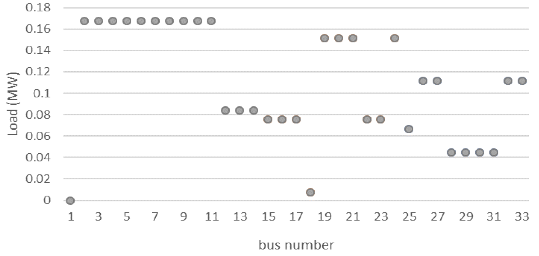
6.1. Reconfiguration for 33-Bus System

Grid search is applied to the 33-bus system. Normally open branches between related buses are detected by reading system data as 33 (8–21), 34 (9–15), 35 (12–22), 36 (18–33) and 37 (25–29). Total active and reactive loads of base system are 3715 kW and 2300 kVAr respectively. Power loss is calculated for the base case as 176.62 kW. In loss calculation GS-1 uses analytical equation (3) and GS-2 run a backward-forward sweep algorithm for power flow analysis for system loads with different load exponents. BIBC matrix is formed, then combinations of tie switches are listed, first one is chosen, and algorithm starts to search. We assume the first tie switch combination is [33-34-35-36-37]. Branch 33 is closed, $\mathit{t}\mathit{m}\mathit{p}$ vector is calculated using the BIBC matrix to identify branches in the loop. The first branch in the loop is opened, BIBC matrix is modified then, second tie switch on line 34 is turned off, second loop is formed and first branch in second loop is opened. BIBC matrix is modified, and the same steps repeated for branches 35 and 36. As the last branch 37 is closed, the last loop is formed, the first branch in the loop is opened, the BIBC is modified and power loss is calculated. Then, all the branches in the last loop are opened one by one and power loss is calculated. Recursive function go one loop back and open the next branch in the previous loop, same search order is repeated for the last loop. Here, the recursive function enables to repeat same steps for every branch in each loop. Thus, power loss for completely changed system topology for each closed-opened branch pair can be calculated.

The optimal open branch configurations for GS-1 and GS-2 are given in

Table 2. The 33-bus system reconfiguration results.

GS-1
Load model	Final configuration	Power loss before reconfiguration (kW)	Power loss after reconfiguration (kW)	CPU time (s)
constant current	7-9-14-32-37	176.37	127.36	19
GS-2
Load exponents	Final configuration	Power loss before reconfiguration (kW)	Power loss after reconfiguration (kW)	CPU time (s)
np = nq = 0 constant power	7-9-14-28-32	202.676	135.385	~170
np = nq = 0.5	7-9-14-28-32	188.676	131.474
np = nq = 1 constant current	7-9-14-32-37	176.628	127.371
np = nq = 1.5	7-9-14-32-37	166.124	122.556
np = nq = 2	7-9-14-32-37	156.872	118.121
np = nq = 2.5	7-9-14-32-37	148.649	114.021
np = nq = 3	7-9-14-32-37	141.279	110.216
np = nq = 3.5	7-9-14-32-37	134.634	106.676
np = nq = 4	7-9-14-31-37	128.611	103.201
np = nq = 4.5	7-9-14-31-37	123.118	99.917
np = nq = 5	7-9-14-31-37	118.087	96.856

. Proposed BIBC modification method is used in both. GS-2 is run for voltage dependent static load models. Here, exponents for load models are chosen between a wide range from 0 to 5 to compare final configurations, power losses before and after reconfiguration with the proposed method GS-1. GS-2 results with $\mathit{n}\mathit{p}=\mathit{n}\mathit{q}=\mathbf{1}$ is for constant current load and give the same results with GS-1 as expected. GS-1 is almost nine times faster than GS-2.

In literature, most of the studies calculate base power loss of 33-bus system as 202.67 kW and optimal configuration as 7-9-14-32-37, which reduces power loss to 139 kW. Minimum bus voltage is 0.913 pu and 0.937 pu before and after reconfiguration, respectively [46,47]. Same base power loss is achieved with constant power load model ($\mathit{n}\mathit{p}=\mathit{n}\mathit{q}=\mathbf{0}$) and exact results obtained via GS-2 is given on Table 2. Configuration of 7-9-14-28-32 reduces losses to 135.38 kW where minimum bus voltage is 0.915 pu after reconfiguration.

Final configuration is the same for most load exponent values, but power loss differs from proposed method GS-1. As voltage dependency increase with higher values of load exponents, final reconfigurations are changed to 7-9-14-31-37. Yet those higher values of load exponents are not typical load characteristics of distribution systems, to swap open branch 31 with 32 also do not cause a big difference in power loss. So, the variation in power loss value depends on the load model rather than the configuration here.

After all, 33-bus system provides the same final configuration as GS-1 for load exponents values from 1 to 3.5 and only one branch changes in final configuration with very small loss reduction for other load exponents. For constant power load model, mostly used in literature, final configuration is same as GS-1 although the exact GS-2 results show that power loss reaches its minimum with a very small reduction when open branch 37 is changed with 28.

In final configuration for higher values of load exponents, 4 to 5, although they are not typical loads for distribution systems, only open branch 32 changes to 31 which do not cause a big topology change. Results for 33-bus system shows proposed method GS-1 with constant current load type approach represents distribution system well and get the results 9 times faster than the GS-2.

6.2. Reconfiguration for 69-Bus System

In 69-bus system, normally open switches are on branches 69 (11–43), 70 (13–21), 71 (15–46), 72 (50–59), 73 (27–65). Total active and reactive loads of base system are 3802 kW and 2694 kVAr, respectively. Active and reactive load levels of 69-bus system are very close to each other. Thus, 69-bus test system is introduced in a capacitor allocation problem in the literature. In order to investigate effects of load types to reconfiguration in such a system, loads are considered only residential, only commercial and only industrial using voltage dependent load formula. Load exponents are chosen from Table 1 for summer season as in

Table 3. The 69-bus system reconfiguration results.

GS-1
Load model	Final configuration	Power loss before reconfiguration (kW)	Power loss after reconfiguration (kW)	CPU time (s)
constant current	14-55-61-69-70	191.50	90.79	216
GS-2
Load exponents	Final configuration	Power loss before reconfiguration (kW)	Power loss after reconfiguration (kW)	CPU time (s)
np = nq = 0 constant power	14-58-61-69-70	224.99	93.44	3341
np = nq = 1 constant current	14-58-61-69-70	191.50	90.79	3429
np = 0.72 nq = 2.96 residential	13-55-61-69-70	181.01	89.39	3580
np = 1.25 nq = 3.50 commercial	13-55-61-69-70	168.46	87.69	3660
np = 0.18 nq = 6.00 industrial	13-55-61-69-70	175.09	87.74	3700

for GS-2. Reconfiguration for the system with constant current and constant power loads is taken into account to compare results with proposed method and studies in literature, respectively.

Final configuration obtained with GS-1 is 14-55-61-69-70. For the constant current loads shown in Table 3, GS-2 gives same power loss of 90.79 kW as GS-1. The difference in final configuration is not essential because it occurs due to sensitive calculations that changes with second open branch. Power loss is changed from 90.7965 to 90.7982 kW by opening branches 58 to 55, respectively. Thus, the final configuration for GS-1 and GS-2 can be accepted as the same due to the unremarkable loss change of 0.0017 kW.

69-bus system has variety of optimal configuration results in literature [48]. The ones with the same power loss of 224.9 kW, have different final power loss values in the range between 96.1 kW and 99.6 kW after reconfiguration. To compare with literature, minimum power loss for constant power load model is calculated in GS-2 as 93.44 kW and final configuration is 14-58-61-69-70. A few numbers of the studies in literature could reached the same configuration with higher final loss value.

Reconfiguration results for 69-bus system with only residential, commercial or industrial loads have the same final configuration and only one branch, 13 instead of 14, is different from the GS-1 solution.

Changing open branch 14 to 13 in GS-1 gives the minimum power loss as 90.87, which is 0.08 kW higher than the exact solution. Therefore, the unlike final configuration can be assumed identical due to very small difference.

Even with the negligible final configuration differences for different load types, in terms of speed, proposed method outperforms with 16 times faster calculation speed for 69-bus system.

6.3. Reconfiguration for Networks with Time Varying Loads

Reconfiguration might be made yearly, monthly, daily or hourly. Switching cost, life of switches and calculation time limits do not provide an opportunity to make optimal switching for each time step in real time. Here, 33-bus system is reorganized with time varying loads. Base active power values of loads at each bus is given in Figure 6. All loads operate at 0.98 power factor. Hourly varied loads are generated using profiles given in Figure 7. Base power are taken as peak values of given time period, 24 h. Industrial and commercial loads reach their peak values in working hours and residential loads in the evening as expected.

Assume there is $\mathit{k}$ number of possible configurations for the system. Grid search estimates power loss, ${\mathit{Ploss}}_i\left(\mathit{t}\right)$ for a specific time. Total power loss of each configuration, $\mathit{Total}\mathit{PowerLos}{\mathit{s}}_{\mathit{i}}$, for the given time period can be calculated as follows:

$$\mathit{Total}\mathit{PowerLos}{\mathit{s}}_{\mathit{i}}=\underset{0}{\overset{\mathit{t}}{{\displaystyle \int }}}{\mathit{Ploss}}_{\mathit{i}}\left(\mathit{t}\right)\mathit{d}\mathit{t} \mathit{i}=\mathit{1}\dots \mathit{k}$$

(12)

The configuration that causes minimum total power loss minimum is accepted as final configuration for the system.

In studies with time varying loads, reconfiguration problem approach generally prioritizes cost minimization rather than only power loss minimization. For a given time period, number of switching operations, cost of switching operations and switching time interval decisions are main concerns of cost calculation beside power loss minimization. However, in this study reconfiguration with time varying loads was examined to see the effects of load modelling in reconfiguration and to validate efficiency of proposed method. For this reason, system loads given in Figure 6 are assumed as only residential, commercial or industrial and load profiles in Figure 7 are used to obtain reconfiguration results both with GS-1 and GS-2 as given in

Table 4. Reconfiguration results of systems with time varying loads.

GS-1
Load type			Final configuration	Power loss before reconfiguration (kW)	Power loss after reconfiguration (kW)	CPU time (s)
residential			9-14-16-27-33	1438.40	875.01	588.1
commercial			9-14-16-27-33	1400.10	851.73	590.6
industrial			9-14-16-27-33	1720.50	1046.60	585.1
GS-2
Load type	Season	Load exponent	Final configuration	Power loss before reconfiguration (kW)	Power loss after reconfiguration (kW)	CPU time (s)
residential	summer/day	np = 0.72 nq = 2.96	9-14-16-27-33	1453.40	877.75	3732.7
	summer/night	np = 0.92 nq = 4.04
	winter/day	np = 1.04 nq = 4.19	9-14-16-27-33	1422.30	870.48	3726.2
	winter/night	np = 1.30 nq = 4.38
commercial	summer/day	np = 0.72 nq = 2.96	9-14-16-27-33	1374.00	846.08	3720.9
	summer/night	np = 0.92 nq = 4.04
	winter/day	np = 1.04 nq = 4.19	9-14-16-27-33	1351.50	840.20	3766.6
	winter/night	np = 1.30 nq = 4.38
industrial	summer/day summer/night winter/day winter/night	np = 0.18 nq = 6.00	9-14-15-28-33	1814.90	1068.32	3880.5

. Different load types with different load exponents for day and night of seasons are given in Table 1. GS-2 is run for each case. Results for residential and commercial load type gave the same configuration as in GS-1. Although the final configuration for system with only industrial loads is different in GS-1 and GS-2, changed open branches does not cause a big topology variation.

As all possible configurations for every time step is calculated with the proposed method, results for each time step or any time interval can also be obtained with given calculation times in Table 4. Proposed method GS-1 is around 6 times faster than GS-2.

7. Discussion

In literature, decision of switch to close/open, control of radiality/continuity, parameter setting of the method, calculation time of power flow analysis, convergence of heuristic or metaheuristic algorithms to local optima are the main challenges of reconfiguration problem. Proposed BIBC matrix modification does not only provide the new topology of network after reconfiguration but also provides the knowledge of formed loops, changed current flow direction. Thus, it enables to examine all switching options with a well organized grid search algorithm without any need to further check radiality/continuity or parameter setting and it gives the exact reconfiguration result which minimize power loss. As proposed method GS-1 assumes network loads as constant current, to compare results and validate method’s effectiveness, a sweep based power flow algorithm, GS-2, is also used in analysis to investigate effect of different load types using a voltage-dependent load model. In

Table 5. Comparison of GS-1 with other methods.

Method	Final Configuration (Opened Switches)	Final Power Loss (kW)	Power Loss Reduction (%)	Min. Bus Voltage (pu)
33 bus system
GS-1	7-9-14-32-37	138.37	31.74	0.9067
GS-2	7-9-14-28-32	135.38	33.2	0.9193
ASFLA [31]	7-9-14-28-32	139.98	30.93	0.9413
CSFSA [49]	7-9-14-32-37	138.91	31.79	0.9423
GWO-PSO [32]	7-9-14-32-37	139.55	31.14	0.9378
SFS [33]	7-9-14-32-37	139.55	31.15	0.9378
ICSA [29]	7-9-14-32-37	139.55	31.15	0.9378
69 bus system
GS-1	14-55-61-69-70	94.07	58.17	0.9594
GS-2	14-58-61-69-70	93.44	58.45	0.9777
ASFLA [31]	14-57-60-61-70	98.59	56.16	0.9459
GWO-PSO [32]	14-57-61-69-70	98.56	56.17	0.9494
SFS [33]	14-55-61-69-70	98.62	56.17	0.9495
ICSA [29]	14-57-61-69-70	98.64	56.15	0.9495

, results are also compared with existing methods in literature. Once the final configuration is obtained by GS-1, final power loss is recalculated using a backward-forward sweep algorithm to be able to compare with other methods which use conventional power flow analysis. Also, loads are modelled as constant power in GS-2 which gives the exact solution of reconfiguration problem by trying all configuration options with grid search.

For 33-bus and 69-bus systems with various load types, final configurations are identical or very similar to proposed method GS-1 as presented in Section 6.1 and Section 6.2. Moreover, the 33-bus system with time varying loads is tested using voltage dependent residential, commercial and industrial loads that differs during the day for each season. The results demonstrate the effectiveness of proposed approach for residential and commercial loads by using various load exponents for voltage-dependent loads in GS-2 analysis which give the same final configuration as GS-1. Effects of various reactive load exponents might not be essential because distribution system loads commonly operate with power factors close to 1, which cause small values of reactive power, but the difference in final configuration for industrial loads may occur due to very high reactive load exponents with an almost zero active load exponent. Overall, various load types are considered separately to see the difference with the constant current load approach in the proposed method. In actual distribution networks that need to balance residential, commercial and industrial loads together, the proposed method can be applied as discussed above.

In terms of calculation time, according to analysis of 33-bus and 69-bus systems and systems with time varying loads, as number of possible switching options increase, spent time to examine all options also gets longer. Proposed method with grid search find the final network topology of 33-bus system with minimum power loss in almost 20 s while calculation time rise to 216 s for 69-bus system. Yet in any case, compare to results with power flow analysis, calculation time of proposed method GS-1 is 9 times faster for 33-bus system, 16 times faster for 69-bus system and almost 7 times faster for systems with time varying loads. While grid search is quite convenient to be used as an exact solution method in distribution network reconfiguration for 33-bus and 69-bus systems, it may not be possible to achieve results in reasonable duration for larger and more complicated systems. Proposed BIBC modification method for network topology change allows estimation of power loss with analytical expression instead of power flow analysis and it is possible to implement the method in any other search algorithms to shorten the execution time.

8. Conclusions

This paper has presented a method for BIBC matrix modification to represent network topology changes. Proposed method is implemented in distribution network reconfiguration problem to get an exact solution. An analytical expression was used to calculate power loss based on BIBC matrix and bus current injections. Reconfigured topology and power loss of network are obtained with the proposed modification of the BIBC matrix, which ensures radiality and continuity of system. Final configuration for the minimum power loss is reached with a grid search algorithm that examines all possible switching operations using a recursive function. Proposed method assumes system loads as constant current injections thus validation of method is verified by analyzing systems with voltage dependent load models using a sweep algorithm based power flow analysis. For voltage dependent load model, various load exponents are tested to investigate effects of load types. As distribution system loads operate at power factor close to unity, higher reactive load exponents do not affect results substantially.

According to the results, constant current approach used in proposed method could represent most of the distribution network loads and it is highly reliable for residential and commercial loads. It might be less efficient for systems with high level of industrial loads because characteristics of industrial loads tend to close constant power with higher reactive load impact and might cause different reconfiguration results. Although calculation time certainly depends on the system topology rather than the size of network, a small system with same number of switches that creates longer loops may have equal possible switching options of a big system with same number of switches which creates very small loops, it is verified that using proposed analytical loss calculation formula instead of power flow analysis (considering the exact solution method examines each possible switching option), substantially reduces the calculation time. As presented in this work, the method for modification of BIBC matrix has made it possible to use in different applications like reconfiguration. Furthermore, reconfiguration strategy with proposed BIBC modification which gives the information of possible topologies after closing a tie switch removes the necessity of radiality/continuity check constraint of the problem. The proposed BIBC modification method, that needs only initial network topology information, is a practical tool for reconfiguration studies with any search method or heuristic/meta-heuristic optimization algorithm.

References

1. Di Fazio, A.R.; Russo, M.; Valeri, S.; de Santis, M. Linear method for steady-state analysis of radial distribution systems. Int. J. Electr. Power Energy Syst. 2018, 99, 744–755. [Google Scholar] [CrossRef]
2. Teng, J.H. A direct approach for distribution system load flow solutions. IEEE Trans. Power Deliv. 2003, 18, 882–887. [Google Scholar] [CrossRef]
3. Garces, A. A Linear Three-Phase Load Flow for Power Distribution Systems. IEEE Trans. Power Syst. 2016, 31, 827–828. [Google Scholar] [CrossRef]
4. Wang, Y.; Zhang, N.; Li, H.; Yang, J.; Kang, C. Linear three-phase power flow for unbalanced active distribution networks with PV nodes. CSEE J. Power Energy Syst. 2017, 3, 321–324. [Google Scholar] [CrossRef]
5. Ayres, H.M.; Salles, D.; Freitas, W. A practical second-order based method for power losses estimation in distribution systems with distributed generation. IEEE Trans. Power Syst. 2014, 29, 666–674. [Google Scholar] [CrossRef]
6. Gözel, T.; Hocaoglu, M.H. An analytical method for the sizing and siting of distributed generators in radial systems. Electr. Power Syst. Res. 2009, 9, 912–918. [Google Scholar] [CrossRef]
7. Ahmadi, H.; Martí, J.R. Distribution system optimization based on a linear power-flow formulation. IEEE Trans. Power Deliv. 2015, 30, 25–33. [Google Scholar] [CrossRef]
8. Oshnoei, A.; Khezri, R.; Hagh, M.T.; Techato, K.; Muyeen, S.M.; Sadeghian, O. Direct probabilistic load flow in radial distribution systems including wind farms: An approach based on data clustering. Energies 2018, 11, 310. [Google Scholar] [CrossRef] [Green Version]
9. Eminoglu, U.; Gözel, T.; Hocaoglu, M.H. DSPFAP: Distribution systems power flow analysis package using matlab graphical user interface (GUI). Comput. Appl. Eng. Educ. 2010, 18, 1–13. [Google Scholar] [CrossRef]
10. Parihar, S.S.; Malik, N. Power flow analysis of balanced radial distribution system with composite load model. In Proceedings of the 2017 Recent Developments in Control, Automation and Power Engineering, RDCAPE 2017, Noida, India, 26–27 October 2017. [Google Scholar]
11. Teng, J.H. Integration of distributed generators into distribution three-phase load flow analysis. In Proceedings of the 2005 IEEE Russia Power Tech, PowerTech, St. Petersburg, Russia, 27–30 June 2005. [Google Scholar]
12. Bazrafshan, M.; Gatsis, N. Comprehensive Modeling of Three-Phase Distribution Systems via the Bus Admittance Matrix. IEEE Trans. Power Syst. 2018, 33, 2015–2029. [Google Scholar] [CrossRef] [Green Version]
13. Memon, Z.A.; Trinchero, R.; Xie, Y.; Canavero, F.G.; Stievano, I.S. An Iterative Scheme for the Power-Flow Analysis of Distribution Networks based on Decoupled Circuit Equivalents in the Phasor Domain. Energies 2020, 13, 386. [Google Scholar] [CrossRef] [Green Version]
14. Cetindag, B.; Kocar, I.; Gueye, A.; Karaagac, U. Modeling of Step Voltage Regulators in Multiphase Load Flow Solution of Distribution Systems Using Newton’s Method and Augmented Nodal Analysis. Electr. Power Components Syst. 2017, 45, 1667–1677. [Google Scholar] [CrossRef]
15. Teng, J.H.; Lu, C.N. Feeder-switch relocation for customer interruption cost minimization. IEEE Trans. Power Deliv. 2002, 17, 254–259. [Google Scholar] [CrossRef]
16. Baran, M.E.; Wu, F.F. Network reconfiguration in distribution systems for loss reduction and load balancing. IEEE Trans. Power Deliv. 1989, 17, 254–259. [Google Scholar]
17. Shi, Q.; Li, F.; Olama, M.; Dong, J.; Xue, Y.; Starke, M.; Winstead, C.; Kuruganti, T. Network reconfiguration and distributed energy resource scheduling for improved distribution system resilience. Int. J. Electr. Power Energy Syst. 2021, 124, 106355. [Google Scholar] [CrossRef]
18. Raoufi, H.; Vahidinasab, V.; Mehran, K. Power systems resilience metrics: A comprehensive review of challenges and outlook. Sustainability 2020, 12, 9698. [Google Scholar] [CrossRef]
19. Sambaiah, K.S.; Jayabarathi, T. Loss minimization techniques for optimal operation and planning of distribution systems: A review of different methodologies. Int. Trans. Electr. Energy Syst. 2019, 30. [Google Scholar] [CrossRef] [Green Version]
20. Shirmohammadi, D.; Hong, H.W. Reconfiguration of electric distribution networks for resistive line losses reduction. IEEE Trans. Power Deliv. 1989, 4, 1492–1498. [Google Scholar] [CrossRef]
21. Civanlar, S.; Grainger, J.J.; Yin, H.; Lee, S.S.H. Distribution Feeder Reconfiguration for Loss Reduction. IEEE Trans. Power Deliv. 1988, 3, 1217–1223. [Google Scholar] [CrossRef]
22. Goswami, S.K.; Basu, S.K. A new algorithm for the reconfiguration of distribution feeders for loss minimization. IEEE Trans. Power Deliv. 1992, 7, 1484–1491. [Google Scholar] [CrossRef]
23. Nara, K.; Shiose, A.; Kitagawa, M.; Ishihara, T. Implementation of Genetic Algorithm for Distribution Systems Loss Minimum Re-Configuration. IEEE Trans. Power Syst. 1992, 7, 1044–1051. [Google Scholar] [CrossRef]
24. Su, C.T.; Chang, C.F.; Chiou, J.P. Distribution network reconfiguration for loss reduction by ant colony search algorithm. Electr. Power Syst. Res. 2005, 75, 190–199. [Google Scholar] [CrossRef]
25. Rao, R.S.; Narasimham, S.V.L.; Raju, M.R.; Rao, A.S. Optimal network reconfiguration of large-scale distribution system using harmony search algorithm. IEEE Trans. Power Syst. 2011, 26, 1080–1088. [Google Scholar]
26. Abdelaziz, A.Y.; Mohammed, F.M.; Mekhamer, S.F.; Badr, M.A.L. Distribution Systems Reconfiguration using a modified particle swarm optimization algorithm. Electr. Power Syst. Res. 2009, 79, 1521–1530. [Google Scholar] [CrossRef]
27. Kumar, K.S.; Jayabarathi, T. Power system reconfiguration and loss minimization for an distribution systems using bacterial foraging optimization algorithm. Int. J. Electr. Power Energy Syst. 2012, 36, 13–17. [Google Scholar] [CrossRef]
28. Imran, A.M.; Kowsalya, M. A new power system reconfiguration scheme for power loss minimization and voltage profile enhancement using Fireworks Algorithm. Int. J. Electr. Power Energy Syst. 2014, 62, 312–322. [Google Scholar] [CrossRef]
29. Nguyen, T.T.; Nguyen, T.T. An improved cuckoo search algorithm for the problem of electric distribution network reconfiguration. Appl. Soft Comput. J. 2019, 84, 105720. [Google Scholar] [CrossRef]
30. Gerez, C.; Silva, L.I.; Belati, E.A.; Filho, A.J.S.; Costa, E.C.M. Distribution Network Reconfiguration Using Selective Firefly Algorithm and a Load Flow Analysis Criterion for Reducing the Search Space. IEEE Access 2019, 7, 67874–67888. [Google Scholar] [CrossRef]
31. Onlam, A.; Yodphet, D.; Chatthaworn, R.; Surawanitkun, C.; Siritaratiwat, A.; Khunkitti, P. Power loss minimization and voltage stability improvement in electrical distribution system via network reconfiguration and distributed generation placement using novel adaptive shuffled frogs leaping algorithm. Energies 2019, 12, 553. [Google Scholar] [CrossRef] [Green Version]
32. El-salam, M.A.; Beshr, E.; Eteiba, M. A New Hybrid Technique for Minimizing Power Losses in a Distribution System by Optimal Sizing and Siting of Distributed Generators with Network Reconfiguration. Energies 2018, 11, 3351. [Google Scholar] [CrossRef] [Green Version]
33. Tran, T.T.; Truong, K.H.; Vo, D.N. Stochastic fractal search algorithm for reconfiguration of distribution networks with distributed generations. Ain Shams Eng. J. 2020, 11, 389–407. [Google Scholar] [CrossRef]
34. Milani, A.E.; Haghifam, M.R. An evolutionary approach for optimal time interval determination in distribution network reconfiguration under variable load. Math. Comput. Model 2013, 57, 68–77. [Google Scholar] [CrossRef]
35. Chidanandappa, R.; Ananthapadmanabha, T.; Ranjith, H.C. Genetic Algorithm Based Network Reconfiguration in Distribution Systems with Multiple DGs for Time Varying Loads. Procedia Technol. 2015, 21, 460–467. [Google Scholar] [CrossRef] [Green Version]
36. Zhan, J.; Liu, W.; Chung, C.Y.; Yang, J. Switch Opening and Exchange Method for Stochastic Distribution Network Reconfiguration. IEEE Trans. Smart Grid 2020, 11, 2995–3007. [Google Scholar] [CrossRef]
37. Teimourzadeh, H.; Mohammadi-Ivatloo, B. A three-dimensional group search optimization approach for simultaneous planning of distributed generation units and distribution network reconfiguration. Appl. Soft Comput. 2020, 88, 106012. [Google Scholar] [CrossRef]
38. Xing, H.; Sun, X. Distributed generation locating and sizing in active distribution network considering network reconfiguration. IEEE Access 2017, 5, 14768–14774. [Google Scholar] [CrossRef]
39. Amin, A.; Tareen, W.U.K.; Usman, M.; Memon, K.A.; Horan, B.; Mahmood, A.; Mekhilef, S. An integrated approach to optimal charging scheduling of electric vehicles integrated with improved medium-voltage network reconfiguration for power loss minimization. Sustainability 2020, 12, 9211. [Google Scholar] [CrossRef]
40. Chen, Q.; Wang, W.; Wang, H.; Wu, J.; Li, X.; Lan, J. A Social Beetle Swarm Algorithm Based on Grey Target Decision-Making for a Multiobjective Distribution Network Reconfiguration Considering Partition of Time Intervals. IEEE Access 2020, 8, 204987–205013. [Google Scholar] [CrossRef]
41. Teimourzadeh, S.; Zare, K. Application of binary group search optimization to distribution network reconfiguration. Int. J. Electr. Power Energy Syst. 2014, 62, 461–468. [Google Scholar] [CrossRef]
42. Thukaram, D.; Banda, H.M.W.; Jerome, J. Robust three phase power flow algorithm for radial distribution systems. Electr. Power Syst. Res. 1999, 50, 227–236. [Google Scholar] [CrossRef]
43. Iliceto, F.; Ceyhan, A.; Ruckstuhl, G. Behavior of loads during voltage dips encountered in stability studies. Field and laboratory tests. IEEE Trans. Power Appar. Syst. 1972, PAS-91, 2470–2479. [Google Scholar]
44. Vaahedi, E.; Fl-Kady, M.A.; Libaque-Esaine, J.A.; Carvelho, V.F. Load Models for Large-Scale Stability Studies from End-User Consumption. IEEE Trans. Power Syst. 1987, 2, 864–870. [Google Scholar] [CrossRef]
45. Baran, M.E.; Wu, F.F. Optimal capacitor placement on radial distribution systems. IEEE Trans. Power Deliv. 1989, 4, 725–734. [Google Scholar] [CrossRef]
46. Ramos, E.R.; Expósito, A.G.; Santos, J.R.; Iborra, F.L. Path-based distribution network modeling: Application to reconfiguration for loss reduction. IEEE Trans. Power Syst. 2005, 20, 556–564. [Google Scholar] [CrossRef]
47. McDermott, T.E.; Drezga, I.; Broadwater, R.P. A heuristic nonlinear constructive method for distribution system reconfiguration. IEEE Trans. Power Syst. 1999, 14, 478–483. [Google Scholar] [CrossRef]
48. Mishra, S.; Paul, S.; Das, D. A comprehensive review on power distribution network reconfiguration. Energy Syst. 2016, 8, 227–284. [Google Scholar] [CrossRef]
49. The, T.T.; Ngoc, D.V.; Anh, N.T. Distribution Network Reconfiguration for Power Loss Reduction and Voltage Profile Improvement Using Chaotic Stochastic Fractal Search Algorithm. Complexity 2020, 2020, 1–15. [Google Scholar]
Figure 1. The 6-bus system base configuration (a) and BIBC matrix (b).
Energies 14 02738 g001
Figure 2. The 6-bus system mesh configuration (a) and BIBC matrix (b).
Energies 14 02738 g002
Figure 3. The 6-bus system new configuration (a) and BIBC matrix (b).
Energies 14 02738 g003
Figure 4. The BIBC and rBIBC matrix.
Energies 14 02738 g004
Figure 5. Flowchart of grid search algorithm.
Energies 14 02738 g005
Figure 6. The 33-bus system load distribution.
Energies 14 02738 g006
Figure 7. The 33-bus system normalized load profile.
Energies 14 02738 g007