Systematic Method for the Energy-Saving Potential Calculation of Air Conditioning Systems via Data Mining. Part II: A Detailed Case Study

 ,
,
Abstract
:1. Introduction
2. Methodology
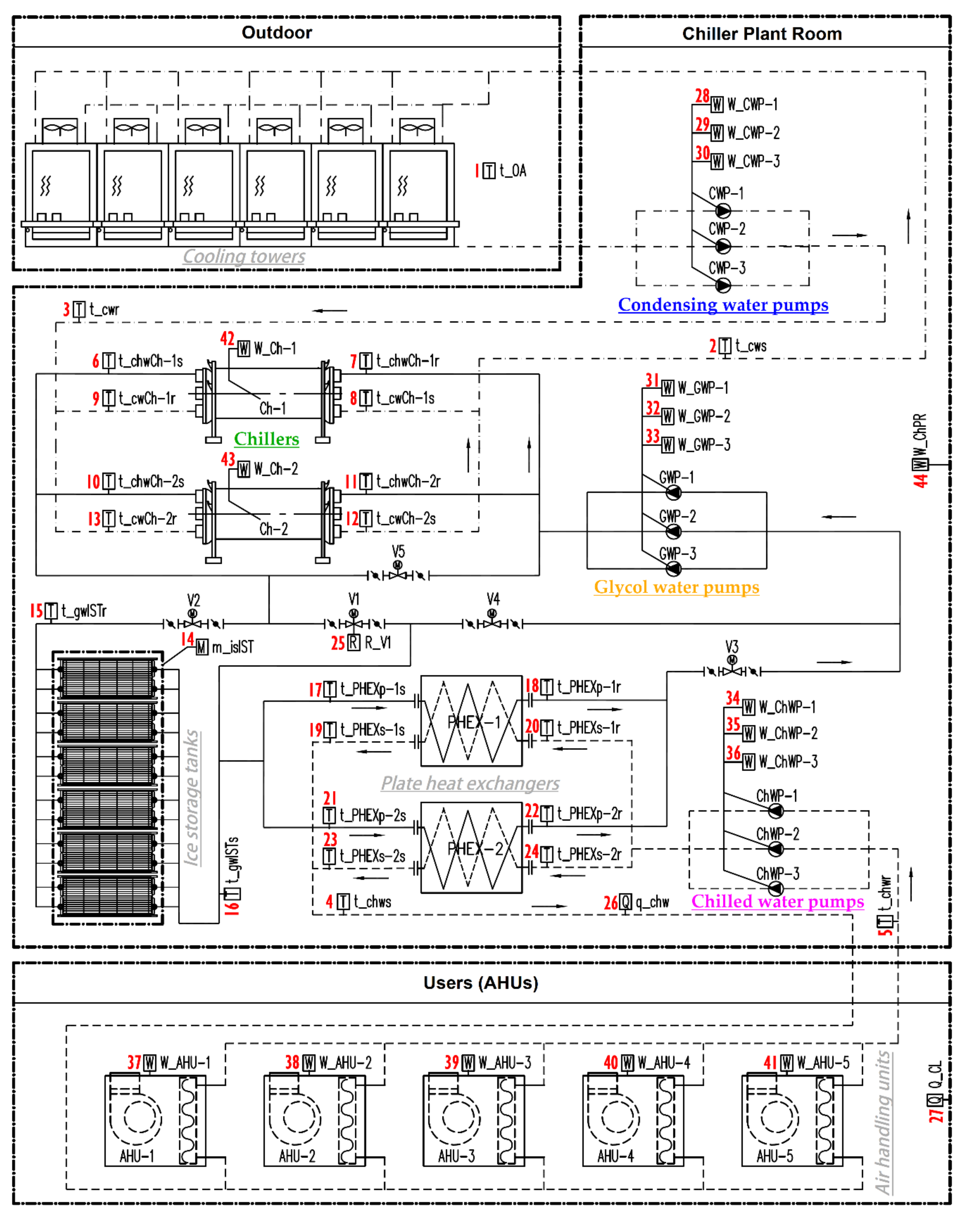
2.1. The Studied System
2.2. Data Collection
2.3. Data Preprocessing
2.3.1. Missing Data Preprocessing
- Listwise deletion: We deleted the data obtained before 22 June 2013, owing to abundant missing values in the data from that period. This was done to ensure the continuity, isometry, and completeness of the data. Consequently, 1416 pairs of continuous time-series data for 59 consecutive days from 22 June to 19 August 2013 were retained for the recognition of system operation mode in Section 2.5 and the energy cost-savings potential analysis in Section 2.8.
- Pairwise deletion: In the regression analysis (Section 2.6) of energy consumption and flow rate for pumps, we deleted the energy-consumption data and the paired flow rate data in cases where either one or both values were missing. The same approach was applied to the data used in the regression analysis for the chillers.
2.3.2. Data Cleaning
- Duplicate data cleaning: Consider the data obtained at 17:59:00 on 18 August 2013 (see Table A2). Because the data were recorded at 1 h intervals, the data obtained at 17:59:00 was considered to be a duplicate of the approaching hour (18:00:00) and was deleted.
- Data cleaning during the shutdown state: To faithfully reflect the distribution of energy consumption in the operating state, before calculating the numerical characteristics of the energy-consumption data of the devices in Section 2.4, the data obtained during the shutdown state (i.e., when the energy consumption was zero) were deleted. The same approach was applied to the data used in Section 2.6 for regression analysis.
2.3.3. Data Extending
- Appending the code of system operation mode to the dataset: Following the recognition of the system operation mode (see Section 2.5), we added a column into the dataset with the corresponding operation-mode code (i.e., M1 to M4 in Table 1 and M0 for the shutdown mode) to facilitate the filtering of data by operation mode in the relevant analysis. For example, the chillers were regressed by cooling (corresponding to M2 and M4) and ice building (corresponding to M1) modes in Section 2.6.
- Temperature difference data extension: Typically, temperature differences are not directly captured and recorded during the data collection period but are frequently used in the analysis. Therefore, it is necessary to add temperature difference data to facilitate direct recall for the relevant analysis (e.g., regression analysis in Section 2.7). For instance, we computed the temperature difference between the supply and the return chilled water (∆tchw = tchwr − tchws) as a new variable (Δtchw) and extended it to the case dataset. Similarly, for the temperature difference of the water supply and return chilled water of the chiller (ΔtchwCh), the temperature difference between the water supply and return condensing water of the chiller (ΔtcwCh) were calculated and extended to the dataset.
2.3.4. Data Transformation
- Transformation of the units of measurement: The unit of the cooling load of the system in the case data was the US refrigeration ton (USRT). This unit pertains to the cooling load (power nature) rather than the cooling quantity demand (energy nature); the former cannot be used directly in the subsequent analysis and calculation. Hence, the unit of USRT was converted to the système international (SI) unit of kilowatts (kW). Because the data collection interval was 1 h, each value corresponded to the cooling quantity demand for that period. Therefore, the unit was further converted to kilowatt-hour (kWh). In the case of chilled water flow (qchw), where there were no more variables of the same type, the unit of liters per second (L/s) was converted to cubic meters per hour (m3/h) to avoid introducing too many conversion factors in the subsequent analysis and calculation.
- Time interval labeling: For easier identification and more efficient data processing, the time interval was marked as period i. The one-to-one correspondences between them are shown in Table A1 of Appendix A.
2.4. Recognition of Variable Speed Equipment
2.5. Recognition of System-Operation Mode
2.6. Regression Analysis of Energy-Consumption Data
2.6.1. Fitting Models for Regression Analysis
2.6.2. Data Preparation for Regression Analysis
- Filter out the flow rate of the individual pump. Considering the chilled water flow rate (qchw) as an example, the data are filtered out with only one chilled water pump in operation from all the data with flow rates (qchw) exceeding zero. The filtered flow data and the corresponding pump energy consumption in the order of pump numbers were used for the respective regression analyses. For instance, a period when ChWP-1 runs while ChWP-2 and ChWP-3 are shut down is determined, chilled water flow rate (qchw) is marked as the flow rate of ChWP-1 (qchw-1), and the process is repeated to filter out the flow rate data for all ChWP-1. Subsequently, these filtered data are organized into a subset of ChWP-1 for regression analysis. The relevant data subsets for ChWP-2 and ChWP-3 can be collated separately following the same procedure.
- Calculate the flow rate of the glycol water (qgw) and the flow rate of the condensing water (qcw). In this study, ignoring the heat transfer loss of the system, Qchw = Qgw, the glycol water flow rate (qgw) can be calculated using the chilled water flow rate (qchw), the temperature difference between supply and return chilled water (Δtchw), and the temperature difference between supply and return glycol water solution (Δtgw) in the operating modes of M2, M3, and M4. Similarly, Qcw = QCh + WCh = Qchw + WCh, the condensing water flow rate (qcw) can be calculated using the chilled water flow rate (qchw), the temperature difference between supply and return chilled water (Δtchw), the energy consumption of the chillers, and the temperature difference between supply and return condensing water (Δtcw) in the operating mode of M2. Finally, using the first method, the relevant data subsets for each glycol water pump and condensing water pump can be collated separately.
2.7. Constraint Analysis of System during Operation
2.7.1. Constraint on Supply and Demand of Cooling
2.7.2. Constraint on Cooling Capacity of Chillers
2.7.3. Constraints on ISTs
2.8. Energy-Saving Potential Analysis
2.8.1. Problem Definition and Principles of Potential Analysis
- For each cooling storage and release cycle, the operation of the air conditioning system shall be optimized and calculated according to the cooling load demand in each period and the constraints described in Section 2.7;
- For each period of a cooling storage and release cycle, the operation mode shall be determined according to the cooling load demand and electricity tariff;
- For each period determined as the operation mode of M4, it is necessary to further determine the respective cooling supply ratios of the ice and chillers;
- For each set of parameters resulting from the above principles, the total energy cost of the chiller plant room was calculated according to the results of the regression analysis in Section 2.6;
- Search for the minimum energy costs as the benchmark energy costs by continuously adjusting the operation mode and other parameters for each period during the cooling storage and release cycle.
- The current remaining cooling capacity in the ISTs at the beginning of period 0 on the first day (i.e., 22 June 2013) is 0 kWh;
- The maximum cooling storage or release speed of ISTs is determined according to the performance curve provided by the manufacturer and the remaining cooling capacity in the ISTs at the beginning of the current period;
- The maximum accumulation of cooling or cooling release of ISTs during one cooling storage and release cycle is determined according to the performance information provided by the manufacturer.
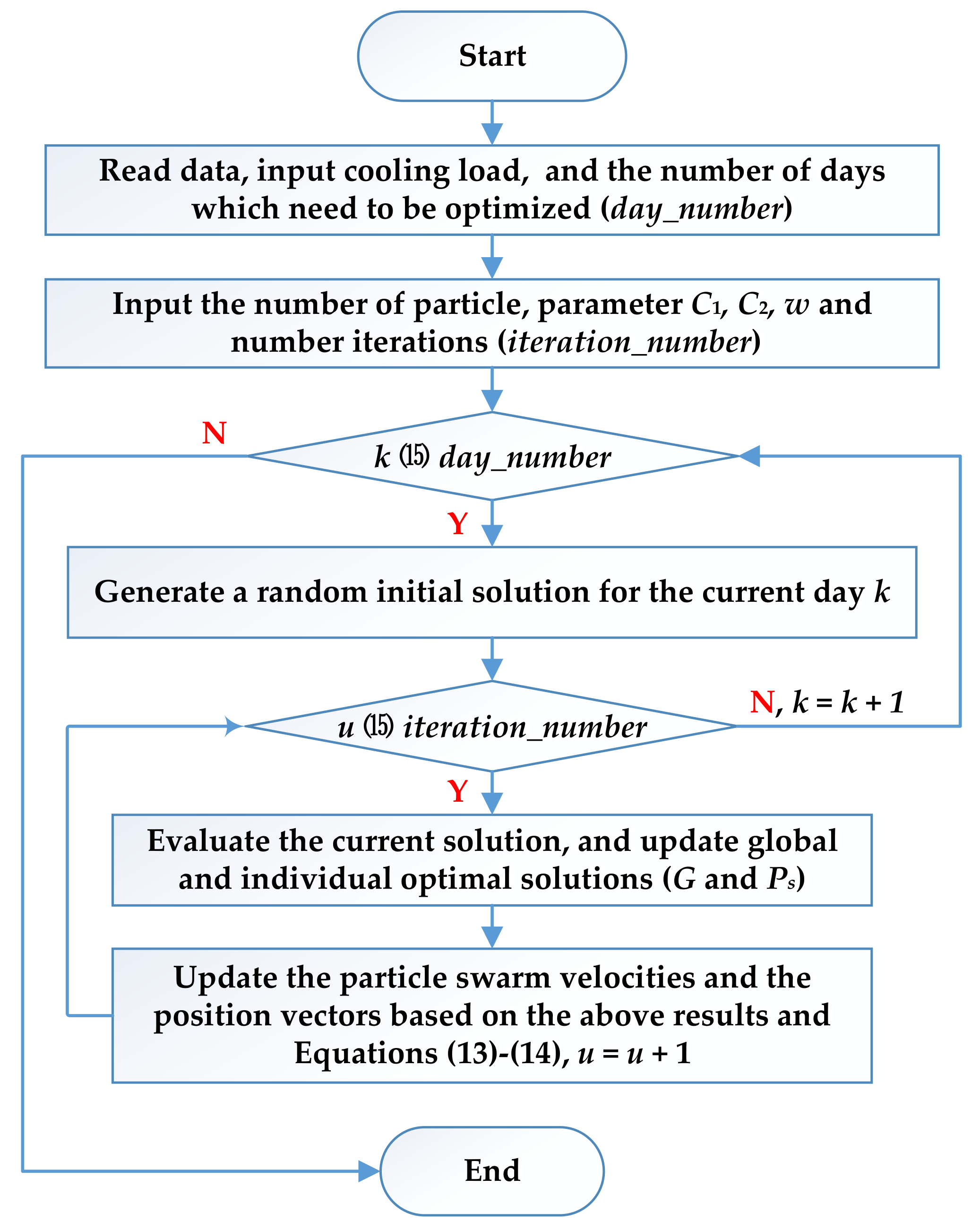
2.8.2. Calculation of the Benchmark Energy Costs by Particle Swarm Optimization (PSO)
- STEP 1: To start, read data from the dataset of the case system, and input the cooling load for each period i of each day and the number of days to be optimized (day_number) into the algorithm by computer:
- STEP 2: Manually input the number of particles, parameters C1, C2, w, and the number of iterations (iteration_number);
- STEP 3: Judge whether the current day k is smaller than day_number; If YES, enter the optimization process of day k, step forward; if NOT, the process ends;
- STEP 4: Generate a random initial solution for the current day k;
- STEP 5: If the iteration (u) for the current day k is smaller than the iteration_number, enter the particle swarm iteration cycle; otherwise, k = k + 1 and step forward to STEP 3;
- STEP 6: Evaluate the current solution and update the global and individual optimal solutions;
- STEP 7: Update the particle swarm velocities and the position vectors based on the results of the previous STEP 6 and in combination with Equations (13) and (14), u = u + 1, and step forward to STEP 5.
- Each solution for the current day k is represented by a position vector Xs;
- The evolution of the solution begins in the PSO with an initial solution consisting of initial particles;
- The initial solution is obtained by a random initial position of each particle; a matrix is employed for recording the operating modes and other status parameters of the case system;
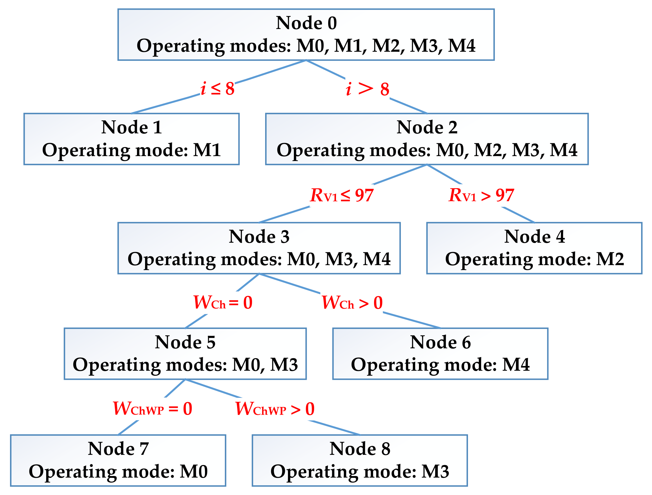
- For the periods 0–8, one of the modes (M0 or M1) can be randomly selected. If M1 is selected, an accumulation of cooling capacity is generated. Call and make sure that Equations (6)–(8) and (11) are valid; otherwise, the mode should be reselected;
- For periods 9–23, one of the modes (M0, M2, M3, or M4) can be randomly selected. However, M0 should be selected as long as = 0. If M2 is selected, call and make sure that Equations (4) and (5) are both valid; otherwise, M4 is selected. If M3 is selected, call and make sure that Equations (4) and (9)–(11) are valid; otherwise, M4 is selected. When M4 is selected, the algorithm randomly generates the respective cooling supply ratio of the ice and chillers. Call and make sure that Equations (4), (5) and (9)–(11) are valid; otherwise, regenerate the respective cooling supply ratio.
3. Results and Discussion
3.1. Recognizing System Running Mode
3.2. Regression Results of ME
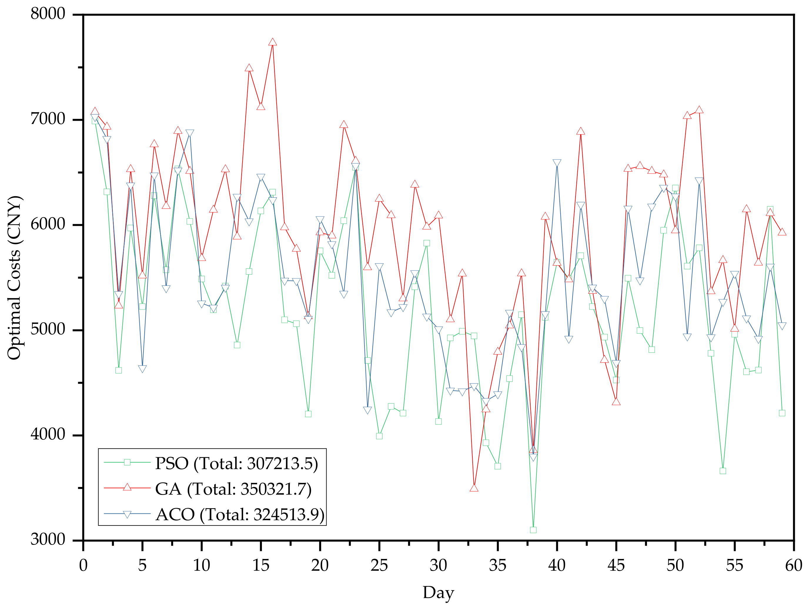
3.3. Energy-Saving Potential Results
3.4. Discussion about Selection of Models
3.5. Advantages of the Systematic Method
3.6. Limitations and Future Outlook
- As previously stated, owing to the lack of sufficient data on cooling towers and terminal AHUs for analysis, the case study could not optimize the energy costs simultaneously in the final optimization. However, this issue does not affect the scientific and systematic nature of the study;
- The final optimization of the method pertained to the whole system rather than the individual devices. This limits the optimization solutions based on the performance of individual devices.
- It is crucial to achieve the energy-saving operation of the air-conditioning system through the improvement of the control strategy, to attain or approach the result of energy-saving potential calculation. Obtaining a set of analysis and operation methods combining potential calculation and optimization control is a practical problem that needs further attention;
- In the research process of diagnostic methods and the employment of these methods to diagnose real air-conditioning systems, the visualization and professional interaction of information and data cannot only improve work efficiency but also have a significant impact on the understanding and application of the relevant results. This is a potential direction for future research.
4. Conclusions
Author Contributions
Funding
Institutional Review Board Statement
Informed Consent Statement
Data Availability Statement
Acknowledgments
Conflicts of Interest
Abbreviations
| ACO | Ant colony optimization |
| AHU | Air handling unit |
| ANN | Artificial neural network |
| CART | Classification and regression trees |
| Ch | Chiller |
| ChWP | Chilled-water pump |
| ChPR | Chiller plant room |
| CWP | Condensing-water pump |
| GA | Genetic algorithm |
| GWP | Glycol water pump |
| HVAC | Heating, ventilating and air conditioning |
| IST | Ice storage tank |
| MAPE | Mean absolute percentage error |
| NN | Neural network |
| OTI | Observation/question, test/calculation, and identification/resolution |
| PHEX | Plate heat exchanger |
| PSO | Particle swarm optimization |
| RSM | Response surface methodology |
| SAX | Symbolic aggregate approximation |
| SI | Système international |
| SVM | Support vector machine |
| USRT | US refrigeration ton |
Appendix A

| i | Time Interval | ei (CNY/kWh) |
|---|---|---|
| 0 | 23:00–00:00 | 0.2884 |
| 1 | 00:00–01:00 | 0.2884 |
| 2 | 01:00–02:00 | 0.2884 |
| 3 | 02:00–03:00 | 0.2884 |
| 4 | 03:00–04:00 | 0.2884 |
| 5 | 04:00–05:00 | 0.2884 |
| 6 | 05:00–06:00 | 0.2884 |
| 7 | 06:00–07:00 | 0.2884 |
| 8 | 07:00–08:00 | 0.8844 |
| 9 | 08:00–09:00 | 0.8844 |
| 10 | 09:00–10:00 | 1.1644 |
| 11 | 10:00–11:00 | 1.1644 |
| 12 | 11:00–12:00 | 1.0244 |
| 13 | 12:00–13:00 | 0.8844 |
| 14 | 13:00–14:00 | 0.8844 |
| 15 | 14:00–15:00 | 1.1644 |
| 16 | 15:00–16:00 | 1.1644 |
| 17 | 16:00–17:00 | 1.0244 |
| 18 | 17:00–18:00 | 0.8844 |
| 19 | 18:00–19:00 | 0.8844 |
| 20 | 19:00–20:00 | 1.1644 |
| 21 | 20:00–21:00 | 1.1644 |
| 22 | 21:00–22:00 | 0.8844 |
| 23 | 22:00–23:00 | 0.8844 |
| Date Time | tOA | tcws | tcwr | tchws | tchwr | tchwCh-1 s | tchwCh-1r | tcwCh-1 s | tcwCh-1r | tgwISTr | tgwISTs | RV1 | qchw | QCL | misIST | WCWP-1 | WCWP-2 | WCWP-3 | WGWP-1 | WGWP-2 | WGWP-3 | WChWP-1 | WChWP-2 | WChWP-3 | WCh-1 | WCh-2 | WChPR |
|---|---|---|---|---|---|---|---|---|---|---|---|---|---|---|---|---|---|---|---|---|---|---|---|---|---|---|---|
| 18 August 2013 00:00:00 | 28.35 | 35.37 | 30.60 | 19.36 | 19.22 | 5.27 | 5.34 | 35.18 | 30.52 | 2.40 | 6.21 | 1.44 | 0.17 | −0.03 | 635.42 | 24.8 | 6.6 | 6.3 | 0 | 26.4 | 40.8 | 0 | 0 | 0 | 261.8 | 257 | 623.7 |
| 18 August 2013 01:00:00 | 28.35 | 33.32 | 30.60 | 19.36 | 19.42 | −0.16 | −0.16 | 33.25 | 30.54 | −2.74 | 0.81 | 1.44 | 0.16 | 0.01 | 623.26 | 24 | 12 | 0 | 0 | 26.4 | 40.8 | 0 | 0 | 0 | 265.6 | 260 | 628.8 |
| 18 August 2013 02:00:00 | 28.25 | 32.82 | 30.30 | 19.46 | 19.52 | −3.33 | −3.35 | 32.79 | 30.18 | −5.74 | −2.36 | 1.44 | 0.16 | 0.01 | 689.52 | 23.9 | 11.9 | 0 | 0 | 26.4 | 40.9 | 0 | 0 | 0 | 266.3 | 252.9 | 622.3 |
| 18 August 2013 03:00:00 | 27.75 | 32.91 | 30.20 | 19.56 | 19.72 | −2.25 | −1.91 | 32.91 | 30.24 | −4.57 | −1.02 | 1.44 | 0.16 | 0.03 | 1626.46 | 23.9 | 11.8 | 0 | 0 | 26.5 | 40.9 | 0 | 0 | 0 | 266.8 | 259.8 | 629.7 |
| 18 August 2013 04:00:00 | 27.95 | 32.91 | 30.30 | 19.56 | 19.82 | −2.54 | −2.27 | 32.96 | 30.30 | −4.77 | −1.36 | 1.44 | 0.16 | 0.05 | 2373.00 | 23.9 | 11.9 | 0 | 0 | 26.4 | 41 | 0 | 0 | 0 | 266.8 | 254.4 | 624.4 |
| 18 August 2013 05:00:00 | 28.05 | 32.91 | 30.30 | 19.66 | 20.02 | −2.79 | −2.51 | 32.96 | 30.30 | −4.98 | −1.63 | 1.44 | 0.16 | 0.07 | 3101.35 | 24 | 11.9 | 0 | 0 | 26.4 | 40.9 | 0 | 0 | 0 | 267.3 | 251.3 | 621.8 |
| 18 August 2013 06:00:00 | 28.05 | 33.01 | 30.41 | 19.66 | 20.12 | −3.03 | −2.81 | 33.02 | 30.42 | −5.27 | −1.88 | 1.44 | 0.16 | 0.09 | 3831.61 | 23.9 | 11.9 | 0 | 0 | 26.5 | 40.9 | 0 | 0 | 0 | 267.9 | 253.8 | 624.9 |
| 18 August 2013 07:00:00 | 28.15 | 32.71 | 30.20 | 19.76 | 20.32 | −3.21 | −2.99 | 32.72 | 30.12 | −5.47 | −2.10 | 1.44 | 0.16 | 0.11 | 4558.58 | 9.9 | 4.9 | 0 | 0 | 10.4 | 16.2 | 0 | 0 | 0 | 101.4 | 93.5 | 236.3 |
| 18 August 2013 08:00:00 | 28.25 | 30.29 | 30.30 | 19.76 | 20.42 | 1.07 | −2.20 | 30.36 | 29.70 | −2.07 | −1.04 | 1.44 | 0.16 | 0.13 | 4574.85 | 0 | 0 | 0 | 0 | 0 | 0 | 0 | 0 | 0 | 0 | 0 | 0 |
| 18 August 2013 09:00:00 | 28.75 | 30.29 | 30.30 | 19.86 | 20.51 | 2.32 | −1.60 | 30.30 | 29.16 | −1.27 | −0.39 | 1.44 | 0.16 | 0.13 | 4542.40 | 0 | 0 | 1.1 | 2.4 | 0 | 0 | 0 | 7.9 | 0 | 0 | 0 | 11.4 |
| 18 August 2013 10:00:00 | 29.25 | 30.09 | 30.30 | 12.73 | 16.78 | 2.86 | −0.87 | 30.06 | 28.86 | 15.73 | 4.46 | 23.10 | 86.37 | 409.84 | 3457.71 | 0 | 0 | 0 | 3.2 | 0 | 0 | 0 | 12.1 | 0 | 0 | 0 | 15.3 |
| 18 August 2013 11:00:00 | 27.55 | 30.09 | 30.30 | 12.04 | 16.45 | 3.82 | −0.21 | 29.82 | 28.62 | 15.37 | 5.38 | 16.48 | 92.78 | 488.93 | 2515.13 | 0.7 | 0 | 0 | 3.3 | 0 | 1.1 | 0 | 12.2 | 1 | 1.2 | 0 | 19.5 |
| 18 August 2013 12:00:00 | 27.55 | 32.84 | 29.24 | 14.84 | 17.75 | 13.73 | 16.88 | 33.38 | 29.21 | 14.43 | 6.22 | 97.57 | 94.33 | 329.83 | 1807.82 | 25.9 | 0 | 0 | 1.5 | 0 | 40.6 | 9.7 | 0 | 6.8 | 262.2 | 17.2 | 363.9 |
| 18 August 2013 13:00:00 | 27.54 | 33.34 | 29.25 | 15.04 | 18.06 | 14.27 | 17.18 | 33.42 | 29.21 | 14.62 | 6.97 | 97.57 | 96.38 | 347.88 | 1821.17 | 25.4 | 0 | 0 | 0 | 0 | 40.8 | 13 | 0 | 0 | 272 | 0 | 351.2 |
| 18 August 2013 14:00:00 | 27.85 | 33.53 | 29.54 | 15.24 | 18.25 | 14.57 | 17.42 | 33.66 | 29.57 | 14.72 | 7.69 | 97.57 | 96.49 | 346.75 | 1843.90 | 10.6 | 0 | 0 | 2.7 | 0 | 16.2 | 6.2 | 7.1 | 0 | 103.1 | 0 | 145.9 |
| 18 August 2013 15:00:00 | 28.25 | 30.76 | 29.64 | 10.23 | 15.16 | 18.99 | 17.51 | 30.00 | 29.39 | 13.59 | 7.01 | 1.52 | 92.02 | 546.69 | 1021.52 | 0 | 0 | 0 | 9.4 | 0 | 0 | 0 | 12.5 | 0 | 0 | 0 | 21.9 |
| 18 August 2013 16:00:00 | 28.55 | 30.66 | 29.64 | 12.15 | 15.98 | 19.65 | 17.15 | 30.00 | 28.79 | 14.61 | 10.22 | 1.52 | 88.76 | 405.65 | 702.72 | 12.1 | 0 | 0 | 5.1 | 0 | 19 | 0 | 5.7 | 14.9 | 96.2 | 0 | 153 |
| 18 August 2013 17:00:00 | 28.95 | 33.83 | 30.02 | 15.63 | 18.69 | 14.90 | 17.85 | 34.14 | 30.03 | 15.40 | 10.33 | 97.44 | 94.69 | 348.18 | 690.35 | 25.7 | 0 | 0 | 1.3 | 0 | 40.5 | 0.3 | 0 | 26.8 | 262.5 | 14.2 | 371.3 |
| 18 August 2013 17:59:00 | 28.95 | 34.23 | 30.33 | 16.35 | 19.29 | 15.57 | 18.51 | 34.46 | 30.33 | 15.50 | 10.74 | 97.44 | 95.95 | 338.33 | 700.05 | 25.1 | 0 | 0 | 0 | 0 | 40 | 0 | 0 | 26 | 263.3 | 0 | 354.4 |
| 18 August 2013 18:00:00 | 28.95 | 34.23 | 30.33 | 16.35 | 19.29 | 15.57 | 18.51 | 34.46 | 30.27 | 15.50 | 10.74 | 97.44 | 97.50 | 343.80 | 700.05 | 25.5 | 0 | 0 | 0 | 0 | 40.7 | 0 | 0 | 26.4 | 267.8 | 0 | 360.4 |
| 18 August 2013 19:00:00 | 28.55 | 33.47 | 30.13 | 16.89 | 19.39 | 18.04 | 19.29 | 30.69 | 30.09 | 15.50 | 11.31 | 97.44 | 103.95 | 311.54 | 709.61 | 26.1 | 0 | 0 | 5 | 0 | 39.3 | 1.6 | 0 | 25.7 | 254.2 | 122.6 | 474.5 |
| 18 August 2013 20:00:00 | 28.24 | 37.26 | 31.31 | 12.67 | 17.25 | 12.62 | 15.07 | 37.05 | 31.39 | 15.50 | 12.11 | 97.44 | 100.74 | 552.70 | 725.60 | 26.6 | 0 | 0 | 8.5 | 0 | 38.4 | 1.8 | 0 | 26.2 | 264.2 | 266.4 | 632.1 |
| 18 August 2013 21:00:00 | 28.14 | 36.96 | 31.21 | 11.67 | 16.24 | 11.74 | 14.05 | 36.70 | 31.21 | 15.59 | 12.33 | 97.44 | 97.30 | 533.77 | 736.38 | 26.5 | 0 | 0 | 8.6 | 0 | 38.3 | 1.8 | 0 | 26.3 | 264.1 | 266.9 | 632.5 |
| 18 August 2013 22:00:00 | 28.14 | 36.76 | 31.21 | 10.87 | 15.34 | 10.97 | 13.20 | 36.64 | 31.15 | 15.79 | 11.83 | 97.44 | 96.02 | 514.53 | 737.41 | 19.1 | 0 | 0 | 6 | 0 | 27 | 1.1 | 0 | 18.9 | 182.1 | 188.4 | 442.6 |
| 18 August 2013 23:00:00 | 28.04 | 31.65 | 31.21 | 13.63 | 13.58 | 14.56 | 13.16 | 31.48 | 30.85 | 16.09 | 11.05 | 1.55 | 0.16 | −0.01 | 713.68 | 14 | 0 | 0 | 0 | 9 | 22.4 | 0 | 0 | 0 | 133.2 | 52.3 | 230.9 |
| Variables | ΔGini |
|---|---|
| i | 0.299 |
| WAHU | 0.276 |
| WChWP | 0.270 |
| WGWP | 0.190 |
| RV1 | 0.188 |
| WCh | 0.172 |
| WCWP | 0.128 |
| Variables | ΔGini |
|---|---|
| RV1 | 0.172 |
| WCh | 0.146 |
| WGWP | 0.137 |
| WChWP | 0.127 |
| WCWP | 0.076 |
| WAHU | 0.056 |
| i | 0.054 |
| Variables | ΔGini |
|---|---|
| WCh | 0.155 |
| WGWP | 0.146 |
| WChWP | 0.140 |
| WCWP | 0.074 |
| WAHU | 0.058 |
| RV1 | 0.054 |
| i | 0.046 |
| Variables | ΔGini |
|---|---|
| WChWP | 0.066 |
| WGWP | 0.063 |
| i | 0.063 |
| WAHU | 0.060 |
| RV1 | 0.029 |
| WCWP | 0.009 |
| WCh | 0.000 |
| Day | Actual Costs (CNY) | Optimal Costs (CNY) | Savings (CNY) | MAPE 1 of Optimal Costs (%) |
|---|---|---|---|---|
| 1 | 9700.0 | 6989.1 | 2710.9 | 2.2% |
| 2 | 8454.8 | 6314.7 | 2140.0 | 3.2% |
| 3 | 6285.1 | 4617.6 | 1667.5 | 7.9% |
| 4 | 6872.3 | 5972.0 | 900.3 | 5.5% |
| 5 | 5893.8 | 5225.0 | 668.8 | 6.6% |
| 6 | 6630.1 | 6278.8 | 351.3 | 3.4% |
| 7 | 6576.5 | 5573.7 | 1002.9 | 2.6% |
| 8 | 8170.0 | 6532.8 | 1637.1 | 5.3% |
| 9 | 7601.2 | 6034.0 | 1567.3 | 5.0% |
| 10 | 6655.7 | 5487.0 | 1168.7 | 4.7% |
| 11 | 6151.9 | 5194.5 | 957.4 | 5.8% |
| 12 | 6955.4 | 5418.4 | 1537.0 | 8.3% |
| 13 | 6749.7 | 4858.5 | 1891.2 | 9.7% |
| 14 | 7610.0 | 5557.6 | 2052.4 | 5.1% |
| 15 | 7752.2 | 6134.0 | 1618.2 | 5.1% |
| 16 | 6933.4 | 6312.6 | 620.8 | 5.5% |
| 17 | 5738.6 | 5097.4 | 641.1 | 9.2% |
| 18 | 5959.4 | 5061.3 | 898.1 | 6.9% |
| 19 | 5695.0 | 4202.9 | 1492.1 | 11.1% |
| 20 | 6376.4 | 5754.5 | 621.9 | 6.0% |
| 21 | 6360.2 | 5521.1 | 839.1 | 6.2% |
| 22 | 7886.9 | 6041.3 | 1845.6 | 4.7% |
| 23 | 8089.9 | 6548.6 | 1541.3 | 3.6% |
| 24 | 7236.2 | 4712.6 | 2523.6 | 4.0% |
| 25 | 5848.2 | 3991.8 | 1856.4 | 8.7% |
| 26 | 6171.7 | 4275.7 | 1896.0 | 8.4% |
| 27 | 6561.4 | 4211.0 | 2350.4 | 7.8% |
| 28 | 6565.0 | 5413.0 | 1152.0 | 3.0% |
| 29 | 6257.1 | 5827.2 | 429.9 | 5.0% |
| 30 | 5990.5 | 4131.1 | 1859.4 | 7.7% |
| 31 | 5866.5 | 4926.2 | 940.3 | 7.1% |
| 32 | 5784.7 | 4989.7 | 795.0 | 6.2% |
| 33 | 5290.7 | 4946.4 | 344.3 | 7.8% |
| 34 | 4995.0 | 3929.5 | 1065.5 | 6.5% |
| 35 | 5258.5 | 3706.8 | 1551.8 | 8.8% |
| 36 | 5983.7 | 4539.1 | 1444.6 | 5.4% |
| 37 | 6654.7 | 5147.4 | 1507.4 | 5.5% |
| 38 | 4439.0 | 3099.5 | 1339.4 | 8.8% |
| 39 | 6745.4 | 5122.6 | 1622.8 | 4.9% |
| 40 | 7495.8 | 5644.6 | 1851.2 | 6.8% |
| 41 | 6366.0 | 5487.9 | 878.1 | 5.1% |
| 42 | 7981.3 | 5707.8 | 2273.5 | 3.9% |
| 43 | 6833.6 | 5224.4 | 1609.3 | 5.9% |
| 44 | 6915.0 | 4934.6 | 1980.4 | 5.9% |
| 45 | 6701.3 | 4525.8 | 2175.5 | 4.6% |
| 46 | 7467.3 | 5494.3 | 1973.0 | 6.7% |
| 47 | 7411.0 | 4997.0 | 2413.9 | 7.0% |
| 48 | 7766.7 | 4815.9 | 2950.9 | 7.9% |
| 49 | 8151.1 | 5949.6 | 2201.4 | 2.6% |
| 50 | 9035.6 | 6352.2 | 2683.4 | 3.7% |
| 51 | 7541.6 | 5608.4 | 1933.2 | 7.1% |
| 52 | 8242.6 | 5783.4 | 2459.2 | 3.4% |
| 53 | 7102.0 | 4780.8 | 2321.2 | 7.9% |
| 54 | 5329.8 | 3661.2 | 1668.5 | 10.1% |
| 55 | 6528.5 | 4962.1 | 1566.4 | 8.7% |
| 56 | 6751.7 | 4605.2 | 2146.5 | 4.8% |
| 57 | 6647.2 | 4621.1 | 2026.1 | 7.4% |
| 58 | 7406.0 | 6149.2 | 1256.8 | 4.9% |
| 59 | 6046.7 | 4211.0 | 1835.7 | 10.2% |
References
- Ma, R.; Wang, X.; Wang, X.-C.; Shan, M.; Yang, X.; Yu, N.; Yang, S. Systematic method for energy saving potential calculation of air conditioning systems via data mining. Part I: Methodology. Energies 2020, 14, 81. [Google Scholar] [CrossRef]
- Zhao, Y.; Zhang, C.; Zhang, Y.; Wang, Z.; Li, J. A review of data mining technologies in building energy systems: Load prediction, pattern identification, fault detection and diagnosis. Energy Built Environ. 2020, 1, 149–164. [Google Scholar] [CrossRef]
- Zhou, Q.; Wang, S.; Xiao, F. A novel strategy for the fault detection and diagnosis of centrifugal chiller systems. HVAC R Res. 2009, 15, 57–75. [Google Scholar] [CrossRef]
- Han, H.; Gu, B.; Kang, J.; Li, Z.R. Study on a hybrid SVM model for chiller FDD applications. Appl. Therm. Eng. 2011, 31, 582–592. [Google Scholar] [CrossRef]
- Van Every, P.M.; Rodriguez, M.; Jones, C.B.; Mammoli, A.A.; Martínez-Ramón, M. Advanced detection of HVAC faults using unsupervised SVM novelty detection and Gaussian process models. Energy Build. 2017, 149, 216–224. [Google Scholar] [CrossRef]
- Yan, R.; Ma, Z.; Zhao, Y.; Kokogiannakis, G. A decision tree based data-driven diagnostic strategy for air handling units. Energy Build. 2016, 133, 37–45. [Google Scholar] [CrossRef]
- Lee, W.Y.; Park, C.; House, J.M.; Kelly, G.E. Fault diagnosis of an air-handling unit using artificial neural networks. ASHRAE Trans. 1996, 102, 540–549. [Google Scholar]
- Magoulès, F.; Zhao, H.; Elizondo, D. Development of an RDP neural network for building energy consumption fault detection and diagnosis. Energy Build. 2013, 62, 133–138. [Google Scholar] [CrossRef]
- Patnaik, D.; Marwah, M.; Sharma, R.; Ramakrishnan, N. Sustainable operation and management of data center chillers using temporal data mining. In Proceedings of the 15th ACM SIGKDD International Conference on Knowledge Discovery and Data Mining, Paris, France, 28 June–1 July 2009; pp. 1305–1314. [Google Scholar]
- Chen, Y.; Wen, J. Whole building system fault detection based on weather pattern matching and PCA method. In Proceedings of the 2017 3rd IEEE International Conference on Control Science and Systems Engineering (ICCSSE), Beijing, China, 17–19 August 2017; pp. 728–732. [Google Scholar]
- Li, G.; Hu, Y.; Chen, H.; Li, H.; Hu, M.; Guo, Y.; Liu, J.; Sun, S.; Sun, M. Data partitioning and association mining for identifying VRF energy consumption patterns under various part loads and refrigerant charge conditions. Appl. Energy 2017, 185, 846–861. [Google Scholar] [CrossRef]
- Li, Z.X.; Renault, F.L.; Gómez, A.O.C.; Sarafraz, M.M.; Khan, H.; Safaei, M.R.; Filho, E.P.B. Nanofluids as secondary fluid in the refrigeration system: Experimental data, regression, ANFIS, and NN modeling. Int. J. Heat Mass Transf. 2019, 144, 118635. [Google Scholar] [CrossRef]
- Sarafraz, M.M.; Tlili, I.; Tian, Z.; Bakouri, M.; Safaei, M.R. Smart optimization of a thermosyphon heat pipe for an evacuated tube solar collector using response surface methodology (RSM). Phys. A Stat. Mech. its Appl. 2019, 534, 122146. [Google Scholar] [CrossRef]
- Sarafraz, M.M.; Safaei, M.R.; Goodarzi, M.; Arjomandi, M. Experimental investigation and performance optimisation of a catalytic reforming micro-reactor using response surface methodology. Energy Convers. Manag. 2019, 199, 111983. [Google Scholar] [CrossRef]
- Rosas-Flores, J.A.; Rosas-Flores, D. Potential energy savings and mitigation of emissions by insulation for residential buildings in Mexico. Energy Build. 2020, 209, 109698. [Google Scholar] [CrossRef]
- Zeng, Y.; Zhang, Z.; Kusiak, A. Predictive modeling and optimization of a multi-zone HVAC system with data mining and firefly algorithms. Energy 2015, 86, 393–402. [Google Scholar] [CrossRef]
- Kwame, A.B.O.; Troy, N.V.; Hamidreza, N. A Multi-Facet Retrofit Approach to Improve Energy Efficiency of Existing Class of Single-Family Residential Buildings in Hot-Humid Climate Zones. Energies 2020, 13, 1178. [Google Scholar] [CrossRef] [Green Version]
- Tian, Z.; Si, B.; Wu, Y.; Zhou, X.; Shi, X. Multi-objective optimization model predictive dispatch precooling and ceiling fans in office buildings under different summer weather conditions. Build. Simul. 2019, 12, 999–1012. [Google Scholar] [CrossRef]
- Ma, R.; Wang, X.; Shan, M.; Yu, N.; Yang, S. Recognition of variable-speed equipment in an air-conditioning system using numerical analysis of energy-consumption data. Energies 2020, 13, 4975. [Google Scholar] [CrossRef]
- Han, J.; Kamber, M.; Pei, J. Data Mining: Concepts and Techniques, 3rd ed.; Elsevier Inc.: Waltham, MA, USA, 2012; ISBN 9780123814791. [Google Scholar]
- Zhang, G.; Chen, L. Opmization of energy consumption in chilled plant. Fluid Mach. 2012, 40, 75–80. [Google Scholar]
- Ma, R. The Study of Energy Efficiency Diagnosis Methodology for Air-Conditioning Systems with the Actual Operating Data. Ph.D. Thesis, Southwest Jiaotong University, Chengdu, China, 2014. [Google Scholar]
- Kennedy, J.; Eberhart, R. Particle Swarm Optimization. In Proceedings of the IEEE International Conference on Neural Networks, Perth, Australia, 27 November–1 December 1995; Volume 4, pp. 1942–1948. [Google Scholar]
- Ma, R.-J.; Yu, N.-Y.; Hu, J.-Y. Application of particle swarm optimization algorithm in the heating system planning problem. Sci. World J. 2013, 2013, 718345. [Google Scholar] [CrossRef] [PubMed] [Green Version]

| Operating Modes | Codes | Device Status | |||||
|---|---|---|---|---|---|---|---|
| Chiller(s) | V1 | V2 | V3 | V4 | V5 | ||
| Ice build | M1 | On | Off | On | Off | On | Off |
| Cooling by chiller(s) only | M2 | On | On | Off | On | Off | Off |
| Cooling by ice only | M3 | Off | Off | On | On | Off | On |
| Cooling by ice with chiller(s) | M4 | On | Modulate | On | On | Modulate | Off |
| No. in Figure 1 | Identifiers in Figure 1 | Parameter Meaning and Unit | Symbol |
|---|---|---|---|
| 1 | t_OA | Outdoor air temperature (°C) | tOA |
| 2 | t_cws | Temperature of supply condensing water in main pipe (°C) | tcws |
| 3 | t_cwr | Temperature of return condensing water in main pipe (°C) | tcwr |
| 4 | t_chws | Temperature of supply chilled water in main pipe (°C) | tchws |
| 5 | t_chwr | Temperature of return chilled water in main pipe (°C) | tchwr |
| 6 | t_chwCh-1 s | Temperature of supply chilled water in chiller #1 (°C) | tchwCh-1 s |
| 7 | t_chwCh-1r | Temperature of return chilled water in chiller #1 (°C) | tchwCh-1r |
| 8 | t_cwCh-1 s | Temperature of supply condensing water in chiller #1 (°C) | tcwCh-1 s |
| 9 | t_cwCh-1r | Temperature of return condensing water in chiller #1 (°C) | tcwCh-1r |
| 10 | t_chwCh-2 s | Temperature of supply chilled water in chiller #2 (°C) | tchwCh-2 s |
| 11 | t_chwCh-2r | Temperature of return chilled water in chiller #2 (°C) | tchwCh-2r |
| 12 | t_cwCh-2 s | Temperature of supply condensing water in chiller #2 (°C) | tcwCh-2 s |
| 13 | t_cwCh-2r | Temperature of return condensing water in chiller #2 (°C) | tcwCh-2r |
| 14 | m_isIST | Amount of ice in inventory (metric tons) | misIST |
| 15 | t_gwISTr | Temperature of return glycol water to ice storage tanks (°C) | tgwISTr |
| 16 | t_gwISTs | Temperature of supply glycol water from ice storage tanks (°C) | tgwISTs |
| 17 | t_PHEXp-1 s | Temperature of supply water to premier side of plate heat exchanger #1 (°C) | tPHEXp-1 s |
| 18 | t_PHEXp-1r | Temperature of return water from premier side of plate heat exchanger #1 (°C) | tPHEXp-1r |
| 19 | t_PHEXs-1 s | Temperature of supply water from secondary side of plate heat exchanger #1 (°C) | tPHEXs-1 s |
| 20 | t_PHEXs-1r | Temperature of return water to secondary side of plate heat exchanger #1 (°C) | tPHEXs-1r |
| 21 | t_PHEXp-2 s | Temperature of supply water to premier side of plate heat exchanger #2 (°C) | tPHEXp-2 s |
| 22 | t_PHEXp-2r | Temperature of return water from premier side of plate heat exchanger #2 (°C) | tPHEXp-2r |
| 23 | t_PHEXs-2 s | Temperature of supply water from secondary side of plate heat exchanger #2 (°C) | tPHEXs-2 s |
| 24 | t_PHEXs-2r | Temperature of return water to secondary side of plate heat exchanger #2 (°C) | tPHEXs-2r |
| 25 | R_V1 | Opening of valve #1 (%) | RV1 |
| 26 | q_chw | Chilled water flow in main pipe (L/s) | qchw |
| 27 | Q_CL | Cooling load of the system (USRT) | QCL |
| 28 | W_CWP-1 | Energy-consumption of condensing water pump #1 (kWh) | WCWP-1 |
| 29 | W_CWP-2 | Energy-consumption of condensing water pump #2 (kWh) | WCWP-2 |
| 30 | W_CWP-3 | Energy-consumption of condensing water pump #3 (kWh) | WCWP-3 |
| 31 | W_GWP-1 | Energy-consumption of glycol water pump #1 (kWh) | WGWP-1 |
| 32 | W_GWP-2 | Energy-consumption of glycol water pump #2 (kWh) | WGWP-2 |
| 33 | W_GWP-3 | Energy-consumption of glycol water pump #3 (kWh) | WGWP-3 |
| 34 | W_ChWP-1 | Energy-consumption of chilled water pump #1 (kWh) | WChWP-1 |
| 35 | W_ChWP-2 | Energy-consumption of chilled water pump #2 (kWh) | WChWP-2 |
| 36 | W_ChWP-3 | Energy-consumption of chilled water pump #3 (kWh) | WChWP-3 |
| 37 | W_AHU-1 | Energy-consumption of air handling unit #1 (kWh) | WAHU-1 |
| 38 | W_AHU-2 | Energy-consumption of air handling unit #2 (kWh) | WAHU-2 |
| 39 | W_AHU-3 | Energy-consumption of air handling unit #3 (kWh) | WAHU-3 |
| 40 | W_AHU-4 | Energy-consumption of air handling unit #4 (kWh) | WAHU-4 |
| 41 | W_AHU-5 | Energy-consumption of air handling unit #5 (kWh) | WAHU-5 |
| 42 | W_Ch-1 | Energy-consumption of chiller #1 (kWh) | WCh-1 |
| 43 | W_Ch-2 | Energy-consumption of chiller #2 (kWh) | WCh-2 |
| 44 | W_ChPR | Energy-consumption of chiller plant room (kWh) | WChPR |
| Operation-Mode Codes | Chiller (s) | Air Handling Unit (s) | Chilled Water Pump (s) | Glycol Water Pump (s) | Condensing Water Pump (s) |
|---|---|---|---|---|---|
| M0 | 0 1 | 0 | 0 | 0 | 0 |
| M1 | >0 2 | 0 | 0 | >0 | >0 |
| M2 | >0 | >0 | >0 | >0 | >0 |
| M3 | 0 | >0 | >0 | >0 | 0 |
| M4 | >0 | >0 | >0 | >0 | >0 |
| Items | Fitting Model | Estimates of Coefficient | Range of Value | ||
|---|---|---|---|---|---|
| β0 | β1 | W (kWh) | q (m3/h) | ||
| ChWP-1 | W = β1 (q + β0)3 | 7.755 | 2.738 × 10⁻⁷ | [7.90, 13.50] | [298.94, 358.92] |
| ChWP-2 | W = β1 (q + β0)3 | −18.501 | 3.475 × 10⁻⁷ | [7.90, 13.80] | [301.79, 359.68] |
| ChWP-3 | W = β0 + β1q | 16.507 | 2.901 × 10⁻² | [25.70, 27.00] | [316.94, 361.76] |
| GWP-1 | W = β1 (q + β0)3 | 136.140 | 7.399 × 10⁻⁸ | [2.00, 6.50] | [163.98, 308.41] |
| GWP-2 | W = β1 (q + β0)3 | 196.989 | 1.785 × 10⁻⁷ | [9.20, 9.80] | [175.14, 183.06] |
| GWP-3 | W = β0 + β1q | 31.554 | 3.558 × 10⁻² | [39.90, 41.30] | [234.58, 273.92] |
| CWP-1 | W = β0 + β1q | 12.541 | 6.148 × 10⁻² | [18.30, 26.60] | [93.67, 228.68] |
| CWP-2 | W = β0 + β1q | 10.236 | 1.416 × 10⁻² | [12.40, 12.70] | [152.76, 173.94] |
| CWP-3 | W = β0 + β1q | 27.410 | 4.928 × 10⁻² | [31.70, 38.40] | [87.04, 222.99] |
| Coefficient | Each Item of the Polynomial | Coefficient Estimate | Standard Error |
|---|---|---|---|
| β0 | 1 | −6630.420 | 1814.984 |
| β1 | QCh | −0.146 | 1.125 |
| β2 | tcwChr | 181.475 | 50.063 |
| β3 | ΔtchwCh | −84.588 | 303.087 |
| β4 | ΔtcwCh | 2,120.110 | 627.771 |
| β5 | (QCh)2 | 8.897×10⁻⁵ | 0.001 |
| β6 | (tcwChr)2 | −1.552 | 0.876 |
| β7 | (ΔtchwCh)2 | 15.478 | 24.417 |
| β8 | (ΔtcwCh)2 | −145.624 | 84.335 |
| β9 | QChtcwChr | −0.020 | 0.030 |
| β10 | QChΔtchwCh | 0.083 | 0.161 |
| β11 | QChΔtcwCh | −0.124 | 0.347 |
| β12 | tcwChrΔtchwCh | 1.965 | 7.730 |
| β13 | tcwChrΔtcwCh | −14.364 | 10.743 |
| β14 | ΔtchwChΔtcwCh | −46.076 | 60.213 |
| β15 | tchwChs | −6.715 | 54.304 |
| β16 | (tchwChs)2 | 0.129 | 0.827 |
| β17 | QChtchwChs | 0.053 | 0.028 |
| β18 | tcwChrtchwChs | −0.705 | 1.517 |
| β19 | ΔtchwChtchwChs | 1.184 | 6.318 |
| β20 | ΔtcwChtchwChs | −10.991 | 14.230 |
| No. | Particle Quantity | Steps of Iterations | Time Cost (s) | Average Result (CNY) |
|---|---|---|---|---|
| 1 | 50 | 50 | 273 | 326,987.4 |
| 2 | 50 | 100 | 541 | 326,311.8 |
| 3 | 50 | 200 | 1 080 | 324,513.9 |
| 4 | 100 | 50 | 544 | 313,138.6 |
| 5 | 100 | 80 | 866 | 309,388.9 |
| 6 | 100 | 100 | 1 083 | 308,598.6 |
| 7 | 100 | 150 | 1 610 | 311,192.5 |
| 8 | 100 | 200 | 2 151 | 310,063.8 |
Publisher’s Note: MDPI stays neutral with regard to jurisdictional claims in published maps and institutional affiliations. |
© 2020 by the authors. Licensee MDPI, Basel, Switzerland. This article is an open access article distributed under the terms and conditions of the Creative Commons Attribution (CC BY) license (http://creativecommons.org/licenses/by/4.0/).
Share and Cite
Ma, R.; Yang, S.; Wang, X.; Wang, X.-C.; Shan, M.; Yu, N.; Yang, X. Systematic Method for the Energy-Saving Potential Calculation of Air Conditioning Systems via Data Mining. Part II: A Detailed Case Study. Energies 2021, 14, 86. https://doi.org/10.3390/en14010086
Ma R, Yang S, Wang X, Wang X-C, Shan M, Yu N, Yang X. Systematic Method for the Energy-Saving Potential Calculation of Air Conditioning Systems via Data Mining. Part II: A Detailed Case Study. Energies. 2021; 14(1):86. https://doi.org/10.3390/en14010086
Chicago/Turabian StyleMa, Rongjiang, Shen Yang, Xianlin Wang, Xi-Cheng Wang, Ming Shan, Nanyang Yu, and Xudong Yang. 2021. "Systematic Method for the Energy-Saving Potential Calculation of Air Conditioning Systems via Data Mining. Part II: A Detailed Case Study" Energies 14, no. 1: 86. https://doi.org/10.3390/en14010086