Abstract
Energy poverty is high up on national and European Union policy agendas. A number of possible indicators to measure the issue have been identified in the literature, but comparable data with European coverage is scarce. The EU Commission thus proposes four independent indicators on the “EU Energy Poverty Observatory” based on self-reported items from the pan-European surveys on income and living conditions (SILC) and household budgets (HBS). It is of increasing public interest to analyse social impacts of energy policies, and quantify energy poverty indicators also from modelling. This paper first shortly outlines how the expenditure-based indicators using HBS micro data may be directly linked to existing macroeconomic models through their defining variables (energy expenditure and income). As endogenous modelling based on micro data is difficult, the link may be country-specific elasticities. The main contribution of the paper is a systematic in-depth sensitivity analysis of the two indicators to changes in income and energy expenditure following varying patterns in the underlying distributions of the micro data. The results may be used by future soft links to models. The results display sometimes counterintuitive effects. We find that whether these indicators increase/decrease after a change of income or energy expenditure largely depends on the specific country-wise income and energy expenditure distribution between households on a micro-level. Due to their definition, the examined indicators are especially sensitive, when income changes alter the indicator threshold values, which in these cases are the median values in underlying distributions. We discuss these findings and relate them to several indicator shortcomings and potential remedies through changes in indicator definition.
1. Introduction
This contribution is an extended version of our paper published at 2020 SDEWES conference, Cologne, Germany [1]. We complemented analyses by additional sensitivity calculations, included respective results chapters and completed interpretations and conclusions.
Energy poverty is not only an issue in a developing country context. The EU Commission [2] (see section “what is energy poverty”) defines it as the inability to access and afford sufficient levels of energy services to fulfil basic needs. Throughout the last two decades, several developments in Europe on both the supply and demand side have aggravated the problem: on the one hand, the financial crisis in 2008 and the related loss of income and assets have impacted the ability of households to pay for energy in several countries [3]. On the other hand, the liberalisation of electricity and gas markets, climate policies, and the transition of energy systems has put an additional economic burden on household budgets, hitting lower-income households particularly hard see e.g., [4,5] (pp. 11–12, 17). Additionally, as a consequence of the deregulation of subsidised prices in some EU Member States (MS), the introduction of energy/CO2-taxes and/or levies and charges for the deployment of renewable energy sources and grid expansion, energy, and the corresponding services have become costlier for households [4,6] (pp. 5, 8–9; 13). Since perceived fairness of societal cost distribution has been found to shape public acceptance of the energy transition [7], the consideration of adverse effects of energy and climate policies on vulnerable households has gained increasing political attention. Accordingly, the ex-ante assessment of social impacts is of increasing importance to ensure a socially just energy transition. In Europe, typically macroeconomic and energy-economic models are applied for impact assessments. Thus, a linking of these with suitable energy poverty indicators is of increasing importance.
1.1. Energy Poverty: Concept and Measurements
There are two broader strands of literature on energy poverty and its measurement. In an international (and especially developing country) context, the view on energy poverty is often related to access to basic energy services and the switching from solid to “modern” fuels (especially electricity and gas; see e.g., [8,9,10,11]. Key publishers in the debate are UN institutions and discussions on corresponding policy targets thus often refer to the sustainable development goals (SDGs).
The second large strand takes a European focus, where electrification rates are close to 100% and the energy infrastructure on average more developed, which shifts the focus to socioeconomic rather than technical barriers to energy access. The concept is also discussed in other world regions, but the literature body is smaller (in the US see e.g., [12], Japan [13], or South Korea [14]).
However, perspectives on and even acknowledgment of the issue across countries have differed a lot in the past so that there still is no European consensus on the concept. Key defining institutions are part of the European Union (EU), national governments, and academia. As this paper focuses on measuring energy poverty in the EU, the below literature review focuses on the European concepts and discussions. Additionally, attempts have been made to reconcile the two strands [15].
The European Commission’s “Energy Poverty Observatory” [2] (see section “what is energy poverty”) defines energy poverty as a state, in which a household (HH) suffers from a lack of adequate domestic energy services (such as heating, cooling, cooking, lighting) for its social and material needs. Energy poverty is a phenomenon with a multitude of influencing factors and manifestations related to national and individual circumstances [16,17] (pp. 25–26, 31; 880, 882), it can be understood and defined in many ways from low living comfort due to inadequate indoor temperature levels to physical and mental health issues as a consequence of mould formation, hypothermia, or social isolation. As a consequence, there is no commonly agreed definition of the issue in Europe (for a discussion of definitions and respective indicators see [5,17,18] (17: pp. 66–72)). Only few EU MS have yet adopted an official energy poverty definition and a smaller number have started developing own indicators/metrics and monitoring them as newly requested by the recasts of the Electricity Directive (2019/944) and the Governance Regulation (2018/1999) adopted within the Clean Energy Package (for an overview of currently employed definitions and metrics in the EU see [19]). Existing official definitions diverge widely and those in the literature have an equally broad range [5,17,19] (pp. 71; 883–885; 9–10), Moore [18] discusses implications of differently defined indicators for the UK. While all try to capture some notion of “energy poverty” and differences may seem semantic at first, these definitions guide the operationalisation and measurement of concepts as a basis for policy making. The key literature [17,19] (pp. 883; 23–24) identifies four main approaches to measurement:
- Expenditure-based metrics define energy poverty based on information about the HH’s expenditure in energy and often compare it to the household’s income;
- Consensual-based metrics use self-reported assessments of indoor housing conditions, and the ability to access and afford basic energy services;
- Direct measurement of the level of energy services (such as heating) achieved in the home compared to a set standard;
- Outcome-based metrics focus on outcomes associated with energy poverty e.g., disconnections, arrears in bill payments, cold-related mortality.
1.2. Key Metrics at EU Level
Each of the above measurement options has its strengths and weaknesses. While the latter two would be of high relevance to capture important energy poverty dimensions, their EU-wide use is hindered by a lack of consistent EU-wide and national-level statistics and limited data access. Consequently, attempts to define and measure energy poverty (such as by the EU Commission [2], OpenExp [20], BPIE [21], and others [22,23]) are mostly based on the former two approaches:
- Expenditure-based metrics are objective measures based on data that is comparable over time and locations but on the other hand do not reflect the causes of expenditure levels. Such indicators are mostly based on the share of income or in absolute energy spending. For defining energy poverty, a normative threshold needs to be set under/above which HHs are considered as energy poor, for absolute spending, share of energy expenses in income or more complex thresholds based e.g., on mean or medians of the population [24,25] (p. 106). Importantly, construct validity of these indicators is debatable [26] (pp. 11–16), since e.g., low absolute energy spending levels may not only indicate poverty (under-consumption) but also be the result of high domestic energy efficiency, and median-based indicators have additional statistical and conceptual drawbacks. Indicator options have been discussed extensively in the literature [17,19,23,24,25,26,27].
- Consensual indicators are based on representative survey data collection. Macro-level indicators are calculated from self-reported (“consensual”) responses. In principle, many dimensions of energy poverty could be captured through this approach. Common questions are on
- ○
- the ability to keep their home adequately warm/cool;
- ○
- whether they have arrears on energy/utility bills;
- ○
- building conditions (the presence of dampness, mould etc.).
Tirado-Herrero [23] (p. 1029) convincingly argues that each indicator has its shortcomings. Accordingly, single fits-all measurements are hardly applicable. Instead multiple metrics capturing different dimensions of energy poverty should be examined in combination and compared to get a complete picture of the status quo.
1.3. Short Review of Energy Poverty Modelling
The goal of this paper is to take a first step towards providing a link for energy poverty indicators to macroeconomic models to allow for an integration of these indicators in future policy impact assessments. We thus first shortly discuss existing energy poverty modelling approaches and in the following section lay down the EU approach to energy expenditure-based metrics.
Across Europe, a number of approaches to explain or model energy poverty outcomes have been proposed that might be used to assess policy impacts by modelling changes to factors found to influence energy poverty levels.
The modelling benchmark in European energy poverty research is the UK Building Research Establishment Domestic Energy Model (BREDEM) [28], which has also been adapted in other EU countries. Their key observation is that “although relatively easy to determine, actual fuel spending is a poor indicator of fuel or energy poverty” [18] (p. 21) because vulnerable HHs often self-ration their energy consumption as they face other pressing needs to be satisfied (e.g., clothes or food) or to avoid falling into debt with utility providers [23] (p. 1023). When for instance poorly insulated buildings are retrofitted, benefits can be realised in terms of energy savings (true for the majority of higher income HHs) or in terms of better indoor conditions and higher temperatures (true for under-consuming lower income HHs). Accordingly, energy efficiency improvements do not necessarily alter fuel expenditure in case of previously existing under-consumption. The model attempts to assess this by technical bottom-up modelling of the housing stock, finding higher theoretical than empirical energy consumption for parts of the population, which is then considered as energy poor [29] (p. 91).
Papada and Kaliampakos [30] apply the official Irish and Scottish energy poverty indicator [31] that is based on the previous Clinch/Healy-approach [29,32] (i.e., modelled fuel costs/income > 10%) to the case of Greece. They model required energy consumption at HH level and then transfer their results to the country level using stochastic Monte Carlo simulation. Not surprisingly, they find income to be the main driver of this energy poverty indicator.
In human geography, spatial drivers of energy poverty have been discussed [33]. For the Netherlands, the determinants of energy poverty were analysed by applying regression analysis to a dataset of 2473 neighbourhoods [34]. While the analysis is enlightening, it remains unclear to what extent drivers of energy poverty are found or rather covariates. Additionally, in the geographical tradition (but beyond Europe), regional “energy poverty scores” of Chinese regions have been analysed [35], but the methodology is not replicable from the explanation. Scrutinised covariates rather seem to conceptually define energy poverty (affordability, income, expenditures) or structure the outcomes (urbanisation) than to explain.
Cambridge Econometrics use a macro econometric model for the UK to assess various policy scenarios on annual energy bill savings for the vulnerable population [36].
In the Energy Performance of Buildings Directive (EPBD) Impact Assessment study for the EU Commission [37], energy poverty impacts were modelled based on survey statistics on the prevalence of energy poverty and assumptions regarding the effectiveness of different energy efficiency policy scenarios (EUCO) to alleviate energy poverty within MS. This approach uses assumptions of policy impacts on underlying micro-data variables to assess macro-level outcomes.
For future impact assessments of the EU, the task will be to include some of the key indicators for energy poverty presented above in existing modelling approaches. Currently employed models are economic and energy-economy models. Dedicated energy poverty modelling as presented in this section is difficult to link to these models. Consensual indicators derived from surveys are also difficult to link: a potential link might be through estimating income-elasticities. However, explanatory power of only income is very low. Expenditure-based metrics as discussed in the literature and which are defined by energy expenditure and income variables only, can directly be linked to macro-economic models without developing full-fledged bottom-up models representing building stocks and replicating empirical vs. theoretical energy (under-)consumption. This has not yet been undertaken in the energy poverty literature body. One way for a soft link to models may be through income and energy expenditure elasticities. A sensitivity analysis of the respective indicators is thus the first step to such a link and for understanding the effects.
1.4. Selection and Definition of Indicators under Analysis
Of the four indicators provided by the EU Energy Poverty Observatory, the two consensual indicators can be calculated and interpreted in a straightforward manner. However, only the two expenditure-based indicators can be potentially linked to macroeconomic models. The expenditure-based indicators used on the EU Energy Poverty Observatory [2] (indicators section) aim at (1) identifying when consumption of basic energy services puts a disproportionate financial burden on HHs in relation to their disposable income or (2) capturing relative under-consumption of basic energy services due to a lack of financial means as described above. Following the literature [19] (p. 25), indicators are defined as
- High share of expenditure in income (HS): percentage of population households whose share of (equivalised) energy expenditure in (equivalised) disposable income is above twice the national median share of energy in income;
- Low absolute expenditure (LA): percentage of population households whose absolute (equivalised) energy expenditure is below half the national median (equivalised) energy expenditure
2. Materials and Methods
2.1. Indicator Generation
The below Table 1 summarises the calculation steps implemented to calculate the two HBS-based energy poverty indicators (HS and LA) as shares of population HHs affected.

Table 1.
Indicator generation: calculation steps.
In order to account for burden differences in varying HH sizes with regard to energy expenditure and marginal utility of disposable HH income, values of both variables have been equivalised using the OECD modified equivalence scale.
Figure 1 shows schematic presentations of how the indicators LA (a) and HS (b) are calculated based on the underlying micro data:
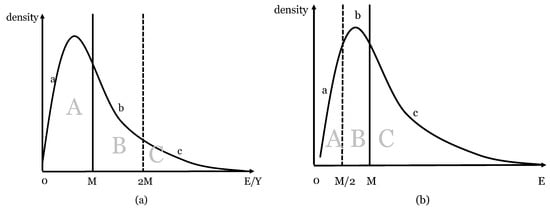
Figure 1.
Schematic representation of HS (a, left) and LA (b, right) indicators.
- (a)
- High share of expenditure in income (HS): the distribution of energy expenditure (E) over income (Y) with the median E/Y value (M) and the indicator threshold (double median, 2M). The “HS” indicator value is the share of the population HHs above the threshold, thus C/(A + B + C). Below, sensitivity effects are discussed as they change key parameters of the distribution and indicator definition.
- (b)
- Low absolute energy expenditure (LA): this section discusses results for sensitivity scenarios along the schematic distribution of low absolute energy expenditure (E) with the median (M) and the indicator threshold (M/2). The LA (“M/2”) indicator value is the share of the population below the threshold, thus A/(A + B + C).
2.2. Database
For the calculation of the expenditure-based indicators, we used the Household Budget Survey (HBS) [38] as the only currently available pan-European database containing the necessary micro data on income and energy expenditure. The HBS is based on nonregulated national data collection by the EU MS, which started in some countries as early as the 1960s and aims at collecting information on expenditure on goods and services. HBS micro data are thus merged from various national data collections, which are not harmonised in frequency, timing, content, and/or structure. Harmonisation of the data is challenging and time consuming and Eurostat only undertakes it in 5-year intervals. So far, only one comprehensive micro data wave (2010) has been released for scientific purposes. This scientific use file does however still not comprise data for all countries, as some have chosen to charge users for its national micro data (AT) or require an additional application via their national statistical office (NL), which complicates full micro data access. Although Eurostat has published “provisional” macro-data based on the newest 2015 wave on Eurobase [39], the release of the 2015 scientific micro data is still pending.
Accordingly, only 2010 data can be currently used, giving a somewhat out-dated perspective on energy poverty in the EU MS. However, it still represents the best data currently available. The complete merged data set comprises all 28 EU MS at the time (including UK), with in total 287,782 observations, and national data sets ranging from 2047 (SE) to 53,996 (DE) observations per country. Due to its unregulated nature, data quality and coverage of relevant variables energy expenditure and income vary between MS despite harmonisation efforts. This concerns particularly household income (the HBS focus lies on expenditure data across different consumption categories). Collection of valid and reliable income data at EU level is instead implemented within the regulated EU Survey on Income and Living Conditions (SILC), which however lacks expenditure data. Relevant variable-specific data gaps and anomalies of HBS data identified in the data preparation process include:
- Income (EUR_HE099): for Italy, no income data is available due to validity concerns following the national data collection process. Accordingly, neither the HS indicator nor income deciles for disaggregation purposes can be calculated for IT. Furthermore, for Luxembourg, reported income components seem to relate to different time units (i.e., per month or per year). Eurostat considers the data unreliable and thus does not use it for publication. Across all countries there are 24,728 observations (i.e., 8.6% of all observations) for which negative income is reported and 22,362 observations (i.e., 7.8% of all observations) for which no income (i.e., income = 0) is reported. Out of these, the majority (22,246) reflect missing data from IT, while the remaining 116 observations are treated as actual income data (i.e., HHs with no income). Furthermore, for Germany there are 698 cases with income values of 1 €, which were also not considered in the analysis.
- Energy expenditure (EUR_HE045): across all countries there are 450 observations (i.e., 0.16% of all observations) for which negative expenditure data is reported and 6014 observations (i.e., 2.1% of all observations) for which no energy expenditure (i.e., energy expenditure = 0) is reported.
While there are possible explanations for negative income values (e.g., payments exceeding annual income, leading to debts) or zero values for energy expenditure (e.g., if energy costs are included in the rent or covered by another party), it is not possible to trace back the origin of these anomalies. For the calculation of indicators, observations with negative income values were deleted.
2.3. Scenarios for Sensitivity Analysis
The purpose of this paper is to analyse the above described expenditure-based indicators as they are defined in the literature [19] and applied by the EU Energy Poverty Observatory [2] (indicators section) regarding their sensitivity to varying patterns in income and energy expenditure development. For this analysis, we define a set of scenarios for income and energy expenditure changes and analyse indicator sensitivities subsequently.
2.3.1. Potential Income Changes
The level of disposable household income influences only the “HS” indicator, as the “LA” indicator is based only on total energy expenditure. Historically, there is a large variety in income change patterns across the EU:
- Income increases are higher in upper income deciles, thus decreasing the share of total income for the lowest decile/quintile (a pattern found for BG, LT, LU by Eurostat [40], for total EU by EIB [41]) or even in combination with decreases of absolute incomes in the lowest deciles (found in Germany by the Deutsches Institut für Wirtschaftsforschung [42] (p. 184)). This is a global pattern found by many scholars, including seminal work and data by Thomas Piketty et al. [43,44].
- No significant change in shares of national income by income quintiles (i.e., even distribution of increases), seen for most EU MS [40,41].
- A redistributive pattern, where lower income classes gain minor shares while higher classes shares are minimally decreasing, and from high levels, as observed for FI, PL, HR, CZ in the 2011-2017 period [40,41], although not likely in the long term and not consistent with other findings (e.g., [44]).
All these varying patterns may happen in the future (at least in certain EU MS) and following the above sources, an effect of +10% income increase (for the entire population, or only in the lower or upper income deciles) may be in a realistic range for a 10-year horizon. We additionally test for indicator sensitivity to 5–20% income changes. We label income as “Y” in graphs and tables. We refer to certain income deciles with “D” and a number [1,10] indicating respective deciles, e.g., D5 for the fifth decile.
2.3.2. Potential Energy Expenditure Changes
HH energy expenditure is a function of energy prices and quantities which both may change over time. It may increase following a rise in prices or energy-relevant activity levels (e.g., increasing floor space heated/capita, larger equipment, etc.) or it may decrease, e.g., due to price decreases, energy efficiency measures, or a decrease in activity levels, i.e., sufficiency actions. Some plausible scenarios include:
- Energy prices may increase significantly, raising costs across all income deciles. For example, official EUCO scenarios [45] (p. 12) project up to 1.2% annual electricity price increases across the EU (EUCO27), and often much higher rates for individual MS.
- Building owners may invest heavily in the energy efficiency of buildings leading to significant decreases in their high building energy consumption and occupants may invest in more efficient equipment decreasing electricity consumption. Such measures are more likely to happen with higher-income classes.
- Additionally, as a consequence of requirements in the EU Energy Efficiency Directive (2018/2002) and Energy Performance of Buildings Directive (2018/844), EU MS may set up targeted and effective programmes that decrease high energy consumption of the vulnerable population via EE measures, i.e., especially of lower-income HHs. In addition, targeted social policies (e.g., direct energy bill payments) may enable low-income HHs to pay a sufficient amount to satisfy their basic energy service needs, which would raise very low energy expenses.
From the above, it seems reasonable to analyse the following medium-term scenarios: (1) energy prices rising by 10%, with accordingly increasing expenditures. (2) Lowering very high (i.e., above double-median) energy expenditures by 10% (as an average, following efficiency measures and targeted policies). (3) An increase of very low (i.e., below half the median) expenditures by 10% (as an average, following targeted policies to the vulnerable and increase in activity levels of wealthier groups). In addition, we analyse sensitivities of 5–20% changes.
We denote energy expenditures as “E”, adding subscripts for especially high “h”, low “l”, or any/all “all” expenditures.
2.3.3. Income and Energy Expenditure Sensitivity Scenarios
A scenario-based projection of income and energy expenditure paths is beyond the scope of this paper. Instead, we analyse the sensitivity of existing indicators to the delineated possible patterns. We thus derive from the above potential futures a set of illustrative combination scenarios and apply these to the HBS micro data. We test the sensitivity of the two indicators (I) to a variation of income (Y) and energy expenditure (E) (see second column of Table 2). With regard to the latter, we test for a variation of decreasing only high expenditures that exceed the double of the national median (Eh), increasing only low energy expenditures that are below half of the national median (El), and of increasing all energy expenditures (Eall). Finally, we test for a joint variation of energy poverty-alleviating changes (increasing income, reducing very high expenditures, and increasing very low expenditures), again for all income groups and lower/higher income half. In addition, we apply these variations to households in all, only in the lower (D1-5), or only in the upper five income deciles (D6-10). The below table shows the variations we test (+/−x%) for all EU MS and the EU in total. We analyse changes of x = 5%, 10%, 15%, and 20% to the respective indicator components.
Table 2.
Sensitivity tests of indicator I, with I = [HS, LA] and x = 5%, 10%, 15%, and 20%.
We apply the sensitivity assumptions as defined in the above sections to the empirical HBS micro data and calculate the effect on the two indicators. The proceeding is straightforward: first, we calculate the indicator values based on the nonaltered HBS 2010 micro data set (status quo). In a second step, we apply the changes: income and energy expenditure data are altered as defined in the scenarios—either for all income deciles or for the lower/upper five income deciles and either all energy expenditures or only very low (below half equivalised national median) or very high (above double equivalised national median) energy expenditures are increased/decreased according to assumptions in Table 2. Calculations are performed for each EU MS separately and for the entire EU. Following Eurostat standard procedures, when defining income deciles at the EU level, deciles are first assigned from national income deciles. Calculations are repeated for the varying levels of change, i.e., 5%, 10%, 15%, and 20%.
3. Results
Results of all sensitivities include data for the (formerly) 28 EU MS and EU total, for two indicators and 15 sensitivity scenarios. Additionally, we provide separate results XLS for the 5%, 10%, 15%, and 20% change sensitivities. These results cannot be presented and discussed exhaustively in this paper. We limit this results section to presenting EU totals and refer to all country findings presented in the full XLS results database (Supplementary Material). We first present key findings of the 10% change sensitivities comparing the different scenarios and provide short explanations of the sometimes counter-intuitive effects. In many cases, effects are due to (changing) underlying national variable distributions in the population. Explanations are given with exemplary distributions (see figures below), while national distributions deviate and may increase/decrease or even revert the effects (see results XLS). In a second step, we present and analyse results of varying the change by 5–20%.
3.1. High Share of Energy Expenses/Income (HS)
This section discusses results for sensitivity scenarios as displayed in Table 3 and Figure 2 for the EU. All EU MS results are provided in the results XLS.
Table 3.
Results of sensitivity scenarios for “high share of expenditure/income” (10% change of indicator components).
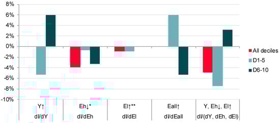
Figure 2.
Results of sensitivity scenarios for HS (10% change of indicator components). * high energy expenditure defined as above twice the national median expenditure. ** under-consumption defined as below half the national median expenditure. Arrows denote an ↑ increase and ↓ decrease.
dHS/dY: a flat-rate increase of Y for all observations leads to a flat-rate decrease of E/Y shares and no change in their distribution, thus there is no change in the indicator. If increases of Y affect only D1-5 HHs, the effect on the indicator is negative, as for these HHs, E/Y-shares are higher (they tend to be at the tail of the distribution in area BC). An increase in Y thus leads to HHs moving from C to B, which reduces the indicator. For D6-10 HHs who tend to have lower shares E/Y (area AB), the left distribution part ab is shifted further left. If HHs move from B to A, M and consequently the HS threshold decrease (effect visible in country effects, see results XLS). Following the HS decrease, more D1-5 HHs at the tail are coded as energy poor without a substantial change to their situation. The total effect depends on the distribution at the tail.
dHS/dEh: reducing very high energy expenditures for all incomes reduces the indicator in all EU MS. The negative effect is found to be substantially stronger when applied to D6-10 HHs than to D1-5 HHs in all MS (except LU). This is due to the applied definition of high energy expenditures (Eh) as more than twice the median expenditures. Such high-expenditures HHs are found mostly in D6-10 and hardly in D1-5. Accordingly, the reduction of Eh affects especially D6-10 HHs. Applied to D1-5 HHs the effect is substantially smaller.
dHS/dEl: an increase of very low energy expenditures defined as below half the national median expenditures (El) leads to a decrease in the indicator. This counterintuitive effect occurs due to the distributional dependency of the indicator. The indicator only changes if an increase in El means also significant change in E/Y (possible for D1-5, but minuscule for D6-10 HHs). Two effects apply here: (1) at least some of the affected HHs are located in the upper end of section A close to M. If these HHs move from A to B, M together with the threshold 2M increase, this is leading to lower indicator values due to HHs being moved from C to B at the tail of the distribution. As a consequence, again the indicator decreases without changing the situation of HHs now labelled “not energy poor”. (2) if HHs have low Eh and at the same time very low incomes (i.e., high E/Y shares), they may shift from B to C, thus increasing the indicator. Empirically we observe a net negative effect for all EU MS apart from AT, DK, and SK, where the net effect is minimally positive. If very low El are increased only for D6-10 HHs, the only minuscule increase of small E/Y (at the very left end of the distribution) causes no change in M nor tail and thus has no effect on the indicator.
dHS/dEall: a change of all energy expenditures (Eall) for all income groups (i.e., right-shifting of distribution abc) has no effect as it does not change the shape of the distribution and increases M by the same percentage. If E increases only for D1-5 HHs, whose shares of E/Y are higher and who tend to be on the right side of the distribution (area BC), their E/Y share further increases and more HHs move from B to C increasing the indicator (see above). The second effect raises the median and thus the threshold value, decreasing the indicator. The net effect is positive when applied to D1-5 HHs (indicator increase) in all EU MS except for FI and SE. For D6-10 HHs who locate more in AB, the net effect is negative (with the exception of SE) without actually changing the situation of the households concerned.
dHS/(dY, dEh, dEl): if a combination of energy-poverty alleviating changes of increasing Y, decrease of high energy expenditures Eh, and increase of low energy expenditures El takes place for all income deciles, this has a net negative effect on the HS indicator (decrease). If only D1-5 HHs are “treated” with the changes, this has a strong negative effect (following above reasons). If only D6-10 HHs benefit from the changes, the income effect increasing the indicator in most countries outweighs the effect of lowered high-expenditures decreasing the indicator. Only in FI, SE, LT, CY, also when only applied to D6-10 HHs a net reducing effect is observed.
3.2. Low Absolute Energy Expenditure (LA)
This section discusses results for sensitivity scenarios along the schematic distribution of low absolute energy expenditure (LA) as presented in Table 4 and Figure 3.
Table 4.
Results of sensitivity scenarios for “low absolute expenditures” (10% change of indicator components).
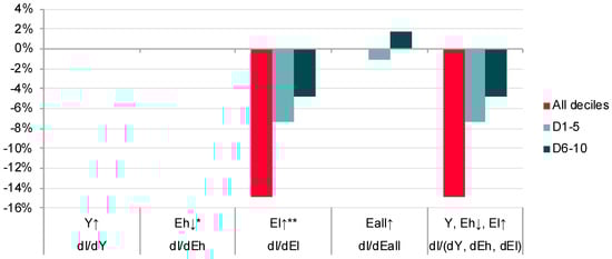
Figure 3.
Results of sensitivity scenarios for LA indicator (10% change of indicator components). * high energy expenditure defined as above twice the national median expenditure. ** under-consumption defined as below half the national median expenditure. Arrows denote an ↑ increase and ↓ decrease.
The LA indicator is defined as household share with absolute energy expenses below half the national median (i.e., area A/(A + B + C) in Figure 1), thus a variation of income Y does not have any effect on the indicator. Equally, if high energy expenses Eh are altered, this changes the distribution at the tail c, but has no effect on the M/2 indicator. Effects can be observed for the other sensitivities:
dLA/dEl: the increase of very low expenditures for all incomes (shifting the distribution a to the right) has by definition a strong negative effect on the indicator (area A decreases due to HHs moving from A to B), while the median M and consequently the threshold M/2 are not altered. If El increases only for D1-5 HHs, who tend to populate area A more, the effect is stronger than for D6-10 HHs who are less represented in area A. Outliers to this effect are IE and UK (see results XLS).
dLA/dEall: if energy expenditures E increase for all incomes, the entire curve abc is shifted to the right, together with M and M/2. As there is no change to the distribution, there is no effect on the indicator A/(A + B + C). If Eall increase only for D1-5 HHs who tend to populate lower expenditure areas AB, more HHs are moving from A to B thus decreasing A and the indicator value. If E increase only for D6-10 HHs who tend to populate higher expenditure areas BC, the distribution a is not changed much, but M and consequently LA may shift to the right thus moving HHs from B to A. This leaves a larger area A increasing indicator values though the situation for these HHs remains unchanged.
dLA/(dY, dEh, dEl): as the LA indicator is independent of Y (dLA/dY = 0) and high energy expenses (dLA/dEh = 0), the combination of changes has the equivalent effect of only changing low expenses (dLA/(dY, dEh, dEl) = dLA/dEl), see above.
3.3. Varying Change: Stability of Sensitivities
As both indicators are calculated applying threshold values that depend on the median of underlying distributions, possible alterations of the threshold values or distributions below/above the thresholds lead to instable indicators. If incomes and energy expenditures rise smoothly for all, little change in indicators is expected. If the changes affect only parts of the distribution and these happen to change the threshold, indicator values may change. Such effects may be nonlinear, i.e., change with varying levels of change. We therefore analyse changes (within the scenarios defined above) of 5%, 10%, 15%, and 20%.
Full results tables for all scenarios and each EU MS are included in the Supplementary Material with one XLS by level of change. Space restrictions limit us to present only total EU findings here (see Figure 4 and Table 5).
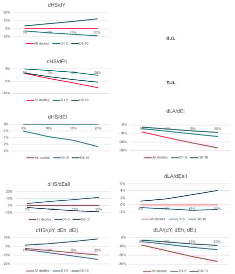
Figure 4.
Sensitivities of HS and LA indicators by scenarios and levels of change. Note: for dHS/dEl, “all decile” values equal D1-5 values and are thus hidden behind the green line.
Table 5.
Sensitivity results for HS and LA indicators, by scenario and variation in change.
We find that the high share of energy expenditure in income (HS) indicator behaves relatively stable across the scenarios and change levels analysed. This of course is contingent on the assumption that only the applied changes to the underlying distributions occur and no other changes take place (ceteris paribus). The changes found resemble the impacts described for the 10% change scenarios in Section 3.1 with the respective explanations.
For the low absolute expenditure (LA) indicator, the scenarios varying only incomes and high energy expenditures have no effect and are thus labelled “n.a.” (as the indicator depends only on low energy expenditures, see Section 3.2). For the three analysed scenarios that do impact the indicator, the sensitivity deviates slightly more from linearity than with the HS indicator. Most significantly, when increasing very low energy expenditures (dEl), the effect on the LA indicator is always negative.
For the combination scenario, again all scenario elasticities remain negative, with elasticities for lower income groups only being higher (negative) than for higher income groups. The combination scenario (dY, dEh, dEl) equals the dEl-scenario, because partial elasticities dY = 0 and dEh = 0, so the only effect in the combination scenario remains dEl.
Interpreting the elasticities in a policy-relevant way, we may draw conclusion on how the HS and LA indicators might react to respective policies. For this, see Section 4.3 below.
4. Discussion
From the sensitivity analysis done in this paper, we observe that in statistical terms, changes to the indicator outcome as an effect of changing income or energy expenditures can be the effect of (1) changes in the distribution curve actually changing the situation of the HHs defined as “energy poor” and (2) as an effect of a changing median and resulting threshold values. The latter can mean a mere “statistical threshold” effect, which is a general drawback of indicators using relative thresholds. To analyse these issues further, a more detailed analysis is necessary regarding which parts of the distribution are empirically populated by which income decile groups and how are these HHs moving within the distribution due to changes to the variables underlying the indicators.
As key question emerges, whether higher income groups (e.g., D6-10 HHs) can actually be considered and should be defined as energy poor, especially when incomes and energy expenditures are already adjusted for household size (via the OECD modified equivalence scale). After all, these HHs should be more able to deliberately increase/decrease energy expenditures (e.g., by energy efficiency measures). At least, a debate on restricting the definition to lower income deciles seems justified. Such a narrowed definition would lower indicator values, but possibly yield more reliable estimates and increase construct validity. Both indicators and effect sizes depend strongly on their underlying national distributions of input variables.
4.1. High Share of Energy Expenditure in Disposable Income (HS)
The HS indicator aims to capture the burden that energy bills put on the household, using the national median as a reference point. Whether a household is considered energy poor depends on the relation between its energy expenditure and disposable income compared to how this measure relates to the national distribution. Consequently, low-income households that under-consume energy services (leading to lower shares of E/Y) are not captured by this indicator. On the other hand, high-income households may be defined as energy poor according to this indicator, if they have a very high energy expenditure. If the key definition of energy poverty is “having limited access to energy services” or “being limited with regard to the consumption of other essential goods or services”, such cases may not fit the definition. As with the LA indicator, the results of the HS indicator depend on its country-level distribution and its median value. This in turn hinges on the distribution of its two components income and energy expenditures.
To limit possible bias that may be introduced by higher-income households (low expenditures due to high efficiency or part-time occupation and a high E/Y share chosen by high-income households that could choose to do otherwise), the definition of “energy poverty” might be restricted to an income threshold, e.g., the population below national median incomes.
In addition, a reduction of indicator values does not necessarily reflect progress: if e.g., low income groups reduce their energy consumption (and thus the HS indicator) below a sustainable level due to a lack of income, a reduction in well-being is wrongfully interpreted as improvement if the assessment is based solely with view to decrease this indicator.
4.2. Low Absolute Energy Expenditure (LA)
The LA indicator considers HHs as energy poor, if energy expenditure is below half the national median value. Consequently, country-specific results depend on the respective distribution of energy expenditures in the lower five expenditure deciles. If the distribution of values is right-skewed, the indicator may yield high shares of energy poor HHs. While such a result may reflect a real problem, there are also alternative explanations to low energy expenditure beyond under-consumption: in some countries (e.g., SE) or cases (e.g., student apartments), energy costs (or a part of them) may be included in the rent and are not captured separately as energy expenditure. Additionally, comparatively low energy expenditure may be the result of higher building and/or appliance energy efficiency, equivocally defining HHs as “energy poor” under the LA definition. If these are high-income HHs, low expenditures actually do not measure under-consumption but wellbeing and may bias the indicator. In addition, in some countries (e.g., DE) parts of energy expenditure of welfare recipients is covered by the state. Interpretation of LA results therefore requires embedding in additional information on national circumstances with regard to building sector characteristics/regulation and social policy.
As a consequence to the definition of the “low absolute expenditures” (LA) indicator, the application of effective energy poverty-alleviating policies that lead to higher energy efficiency in vulnerable groups may lead to increased use of energy services, but not higher expenditure. Such policies would thus not have any effect on the respective indicator. This shows, that the LA indicator alone is not appropriate to capture policy impacts and needs to be accompanied by complementary information.
The HS indicator has also been criticised for applying a supposedly arbitrary threshold of double-mean income that by its introduction equalled a 10% share of energy expenditure in income [44] (p. 11). The threshold would need to be justified with a normative meaning, which is arguably difficult (p. 12). The indicator is criticised for violating “commonly accepted conditions for poverty measurement” (ibid. p. 12) due to its statistical properties such as sensitivity to adding fixed costs (that would reduce the indicator). This implies that rising energy costs may actually reduce the HS indicator. The author therefore argues for the simpler “Ten-Percent [share of energy expenditure in income] -Rule”, or TPR, (ibid, pp. 16–18).
While the calculation of both indicators is relatively straightforward, this does not always apply to the interpretation of outcomes and understanding of effects. Results of the expenditure-based indicators generally have to be interpreted against the background of national circumstances and be complemented by other indicators.
4.3. Discussion of Policy Impacts
The scenarios implemented for this sensitivity analysis may also be seen as effects of potential future policies, such as redistributive polices on incomes (e.g., higher taxation of higher incomes, lower taxation of lower incomes) or on dedicated energy poverty policies using tax or financial allowance instruments (e.g., state coverage of energy bills). Effects can be inferred from sensitivity results (see Figure 4).
An effective redistributive policy raising incomes of low-income groups would lower the HS energy poverty indicator while not affecting at all the LA indicator (which is independent of incomes). Policies that lead to higher income inequality (raising only high incomes) would lead to rising HS indicator levels.
If policies were dedicated to lowering energy costs for those who already have very high expenditures (e.g., through lowering of taxes and levies or energy efficiency improvements only for high-expenditure groups), this would lower HS indicator values. This effect would be stronger, if high-income groups are especially targeted, as they have statistically higher energy expenditures. This hints at a nonbalanced representation of socially vulnerable groups in the indicator. Again, the LA indicator would not be affected (as it is based on low energy costs only).
Policies that aim to raise energy expenditures for those households who currently spend very little on energy would by definition decrease the LA indicator. The effect is stronger for lower income groups as those represent a higher share of low energy-expenditure households. Such policies might include tax/levy refunds or payment of energy bills by state agencies for low-income groups.
If all (low, medium, and high) energy costs rise, e.g., due to rising energy prices or increasing tax/levy levels, this would not alter overall indicator levels (as the entire distribution would be shifted, but relative shares are not changed). However, it would have distributive effects. The HS indicator would rise (fall) in the low (high) income group. For the LA indicator, the effect is inverse: by definition, higher energy bills lower the indicator, which is relatively more pronounced for low-income groups. A decrease of this indicator however has to be interpreted cautiously with regard to energy poverty alleviation, as it rather reflects an aggravation of the situation for the vulnerable households, if bills have to be paid by them.
Finally, a combination of policies that aim at redistributing incomes towards lower-income groups, target cost-reductions for high-cost groups (e.g., through energy efficiency improvements) and aim at raising energy expenses to a sustainable level for under-consuming households (e.g., by covering energy bills from social funds) would lower both indicators. LA indicator values would be lowered in all income groups. The HS indicator however would rise for high incomes, but the effect be overcompensated by strongly falling values for lower incomes leading to a net total decline.
5. Conclusions
For the analyses in this paper, we systematically applied partial changes to incomes and energy expenditures in the national micro data of the HBS for evaluating the resulting changes to the two expenditure-based energy poverty metrics implemented by the EU Energy Poverty Observatory. This sensitivity analysis finds that both indicators provide valuable insights into the state of energy poverty and that changes in the input variables reflect well underlying problems. However, also some mere statistical effects are encountered, when threshold changes lead to indicator changes without improving the situation of the vulnerable population. Such issues might be avoided with a threshold not involving the median but defined in absolute percentage terms [44]. Some countries also exhibit “outlier effects” due to the underlying distributions.
The sensitivity analysis was performed only on the two expenditure-based indicators as defined in the literature and as applied in the EU Energy Poverty Observatory. It thus falls short of discussing these indicators in comparison with other possible energy poverty metrics. This remains as a future research need, then more directed towards the discussion on the various metrics proposed in the literature.
We compared and discussed the sensitivity of the two expenditure-based indicators to a set of scenarios, and analysed variations in change levels of the composing variables energy expenditures and income. We found that effects remain relatively stable across variation levels.
The impacts found can also be interpreted as impacts that future policies affecting energy costs and income distributions have on the two analysed indicators. A general income redistribution policy would have positive impacts on the HS indicator while not affecting the LA indicator. The same is true for policies lowering costs of energy-intensive households e.g., through energy efficiency measures. Any policy that raises energy expenditures that are currently very low would positively alter low absolute expenditure indicator values. Whether this can be interpreted as positive however depends on how this is implemented (rising bills paid by households or state, enabled or forced to pay).
The largest positive effect on both indicators is found for a combination scenario that may follow from a holistic energy poverty policy programme: redistribution of income, lowering high energy costs, and allowing for a sustainable minimum consumption.
The above issues point to the necessity of continuing the academic debate on which indicators are best suited to monitor energy poverty and to assess policy impacts (see e.g., [19,23]). Without engaging in this debate, from the analysis presented in this article we can conclude that a closer national analysis and complementation of the proposed indicators in national cases is needed. Revisiting the definition of indicators for the EU Energy Poverty Observatory and possibly a restriction to lower income deciles seems justified. Still, the two indicators under analysis here in most cases would reflect improvements in the respective covered dimension of energy poverty.
Supplementary Materials
The following are available online at https://www.mdpi.com/1996-1073/14/1/8/s1, XLS files with full sensitivity results by EU member states, for both analysed indicators and all sensitivity scenarios, one file by 5%, 10%, 15%, and 20% sensitivity calculations.
Author Contributions
Conceptualisation, J.T. and F.V.; methodology, J.T. and F.V.; statistical analyses, F.V.; validation, J.T.; investigation, J.T. and F.V.; data curation, F.V.; writing—original draft preparation, J.T.; writing—review and editing, F.V.; visualisation, J.T.; project administration, J.T.; funding acquisition, J.T. All authors have read and agreed to the published version of the manuscript.
Funding
This research received no external funding. It is based on previous research projects (service contracts with the EU Commission) within which authors contributed databases.
Conflicts of Interest
The authors declare no conflict of interest.
Abbreviations
Note: for country references, we use ISO 3166-1 alpha-2 country codes.
| CO2 | Carbon dioxide |
| D# | Decile (# referring to decile 1 to 10) |
| E | Energy expenditure |
| EU | European Union |
| HBS | Household Budget Survey |
| HH | Household |
| HS | High share (of energy expenditure in income indicator) |
| LA | Low absolute (energy expenditure indicator) |
| M | Median |
| MS | Member States |
| SDG | Sustainable Development Goals |
| SILC | Survey on Income and Living Conditions |
| XLS | (MS) Excel table |
| Y | Income |
References
- Thema, J.; Vondung, F. Expenditure-Based Indicators for Measuring Energy Poverty—Sensitivities and Analyses. In SDEWES Conference Proceedings; SDEWES: Zagreb, Croatia, 2020. [Google Scholar]
- EU Commission. EU Energy Poverty Observatory; EU Commission: Brussels, Belgium, 2020. [Google Scholar]
- Dagoumas, A.; Kitsios, F. Assessing the impact of the economic crisis on energy poverty in Greece. Sustain. Cities Soc. 2014, 13, 267–278. [Google Scholar] [CrossRef]
- Frondel, M.; Sommer, S.; Vance, C. The Burden of Germany’s Energy Transition—An Empirical Analysis of Distributional Effects; RWI: Essen, Germany, 2015. [Google Scholar]
- Pye, S.; Dobbins, A.; Baffert, C.; Brajković, J.; Deane, P.; De Miglio, R. Addressing energy poverty and vulnerable consumers in the energy sector across the EU. L’europe En Form. 2015, 378, 64–89. [Google Scholar] [CrossRef]
- European Commission. Energy Prices and Costs in Europe 2020; EU Commission: Brussels, Belgium, 2020. [Google Scholar]
- Perlaviciute, G.; Steg, L. Contextual and psychological factors shaping evaluations and acceptability of energy alternatives: Integrated review and research agenda. Renew. Sustain. Energy Rev. 2014, 35, 361–381. [Google Scholar] [CrossRef]
- Sovacool, B.K. The political economy of energy poverty: A review of key challenges. Energy Sustain. Dev. 2012, 16, 272–282. [Google Scholar] [CrossRef]
- Sovacool, B.K. Energy, Poverty, and Development; Routledge: New York, NY, USA, 2014; Volume 1, ISBN 1-138-01478-8. [Google Scholar]
- Pachauri, S.; Mueller, A.; Kemmler, A.; Spreng, D. On measuring energy poverty in Indian households. World Dev. 2004, 32, 2083–2104. [Google Scholar] [CrossRef]
- Pachauri, S.; Spreng, D. Measuring and monitoring energy poverty. Energy Policy 2011, 39, 7497–7504. [Google Scholar] [CrossRef]
- Bednar, D.J.; Reames, T.G. Recognition of and response to energy poverty in the United States. Nat. Energy 2020, 5, 432–439. [Google Scholar] [CrossRef]
- Okushima, S. Measuring energy poverty in Japan, 2004–2013. Energy Policy 2016, 98, 557–564. [Google Scholar] [CrossRef]
- Jo, H.-H.; Lim, H.-W.; Kim, H.-D. Measuring the Energy Poverty and the Severity in Korea; Economic Research Institute Yonsei University: Seoul, Korea, 2019. [Google Scholar]
- Day, R.; Walker, G.; Simcock, N. Conceptualising energy use and energy poverty using a capabilities framework. Energy Policy 2016, 93, 255–264. [Google Scholar] [CrossRef]
- Simcock, N.; Walker, G.; Day, R. Fuel poverty in the UK: Beyond heating. People Place Policy Online 2016, 10, 25–41. [Google Scholar] [CrossRef]
- Thomson, H.; Bouzarovski, S.; Snell, C. Rethinking the measurement of energy poverty in Europe: A critical analysis of indicators and data. Indoor Built Environ. 2017, 26, 879–901. [Google Scholar] [CrossRef] [PubMed]
- Moore, R. Definitions of fuel poverty: Implications for policy. Energy Policy 2012, 49, 19–26. [Google Scholar] [CrossRef]
- Rademaekers, K.; Yearwood, J.; Ferreira, A.; Pye, S.; Hamilton, I.; Agnolucci, P.; Grover, D.; Karásek, J.; Anisimova, N. Selecting Indicators to Measure Energy Poverty; Trinomics: Rotterdam, The Netherlands, 2016. [Google Scholar]
- OpenExp. European Energy Poverty Index (EEPI) 2020. Available online: https://ec.europa.eu/energy/sites/ener/files/documents/Selecting%20Indicators%20to%20Measure%20Energy%20Poverty.pdf (accessed on 21 December 2020).
- Atanasiu, B.; Kontonasiou, E.; Mariottini, F. Alleviating Fuel Poverty in the EU: Investing in Home Renovation, a Sustainable and Inclusive Solution; Buildings Performance Institute Europe: Brussels, Belgium, 2014. [Google Scholar]
- Thomson, H.; Snell, C. Quantifying the prevalence of fuel poverty across the European Union. Energy Policy 2013, 52, 563–572. [Google Scholar] [CrossRef]
- Tirado Herrero, S. Energy poverty indicators: A critical review of methods. Indoor Built Environ. 2017, 26, 1018–1031. [Google Scholar] [CrossRef]
- Heindl, P. Measuring Fuel Poverty: General Considerations and Application to German Household Data; SOEP Papers on Multidisciplinary Panel Data Research; DIW: Berlin, Germany, 2014. [Google Scholar]
- Hills, J. Fuel Poverty: The Problem and Its Measurement; CASEreport, 69; Department for Energy and Climate Change: London, UK, 2011. [Google Scholar]
- Schuessler, R. Energy Poverty Indicators: Conceptual Issues-Part I: The Ten-Percent-Rule and Double Median/Mean Indicators. SSRN Electron. J. 2014. [Google Scholar] [CrossRef]
- Hills, J. Getting the Measure of Fuel Poverty: Final Report of the Fuel Poverty Review; Centre for Analysis of Social Exclusion, London School of Economics and Political Science: London, UK, 2012. [Google Scholar]
- BRE. BREDEM 2012. A Technical Description of the BRE Domestic Energy Model. Version 1.1; BRE: Watford, UK, 2015. [Google Scholar]
- Clinch, J.P.; Healy, J.D.; King, C. Modelling improvements in domestic energy efficiency. Environ. Model. Softw. 2001, 16, 87–106. [Google Scholar] [CrossRef]
- Papada, L.; Kaliampakos, D. A Stochastic Model for energy poverty analysis. Energy Policy 2018, 116, 153–164. [Google Scholar] [CrossRef]
- DECC. Annual Report on Fuel Poverty Statistics 2011; Department for Energy and Climate Change: London, UK, 2011. [Google Scholar]
- Clinch, J.P.; Healy, J.D. Housing standards and excess winter mortality. J. Epidemiol. Community Health 2000, 54, 719–720. [Google Scholar] [CrossRef]
- Bouzarovski, S.; Simcock, N. Spatializing energy justice. Energy Policy 2017, 107, 640–648. [Google Scholar] [CrossRef]
- Mashhoodi, B.; Stead, D.; van Timmeren, A. Spatial homogeneity and heterogeneity of energy poverty: A neglected dimension. Ann. Gis 2019, 25, 19–31. [Google Scholar] [CrossRef]
- Wang, B.; Li, H.-N.; Yuan, X.-C.; Sun, Z.-M. Energy Poverty in China: A Dynamic Analysis Based on a Hybrid Panel Data Decision Model. Energies 2017, 10, 1942. [Google Scholar] [CrossRef]
- Cambridge Econometrics. Jobs, Growth and Warmer Homes Evaluating the Economic Stimulus of Investing in Energy Efficiency Measures in Fuel Poor Homes; Cambridge Econometrics: Cambridge, UK, 2012. [Google Scholar]
- European Commission E.C. Commission Staff Working Document Impact Assessment: Accompanying the Document Proposal for A Directive of The European Parliament and of the Council Amending Directive 2010/31/EU on the Energy Performance of Buildings; European Commission: Brussels, Belgium, 2016. [Google Scholar]
- Eurostat Household Budget Survey—Eurostat. Available online: https://ec.europa.eu/eurostat/web/microdata/household-budget-survey (accessed on 17 April 2020).
- Eurostat HBS Database. Available online: https://ec.europa.eu/eurostat/web/household-budget-surveys/database (accessed on 17 April 2020).
- Eurostat Living Conditions in Europe—Income Distribution and Income Inequality—Statistics Explained. Available online: https://ec.europa.eu/eurostat/statistics-explained/index.php/Living_conditions_in_Europe_-_income_distribution_and_income_inequality#Income_distribution (accessed on 16 April 2020).
- Bubbico, R.; Freytag, L. Inequality in Europe; European Investment Bank: Luxembourg, 2018. [Google Scholar]
- Grabka, M.M.; Goebel, J. Income distribution in Germany: Real income on the rise since 1991 but more people with low incomes. DIW Wkly. Rep. 2018, 8, 181–190. [Google Scholar]
- Piketty, T.; Goldhammer, A. Capital in the Twenty-First Century; Harvard University Press: Cambridge, MA, USA, 2017; ISBN 978-0-674-97985-7. [Google Scholar]
- WID World Inequality Database. Available online: https://wid.world/ (accessed on 16 April 2020).
- E3MLab; IIASA. Technical Report on Member State Results of the EUCO Policy Scenarios; European Commission: Brussels, Belgium, 2016. [Google Scholar]
Publisher’s Note: MDPI stays neutral with regard to jurisdictional claims in published maps and institutional affiliations. |
© 2020 by the authors. Licensee MDPI, Basel, Switzerland. This article is an open access article distributed under the terms and conditions of the Creative Commons Attribution (CC BY) license (http://creativecommons.org/licenses/by/4.0/).