Investigating Fourteen Countries to Maximum the Economy Benefit by Using Offline Reconfiguration for Medium Scale PV Array Arrangements

 ,
,  , ,
, ,  and
and 
Abstract
1. Introduction
2. Electrical Characteristics of Photovoltaics (PVs)
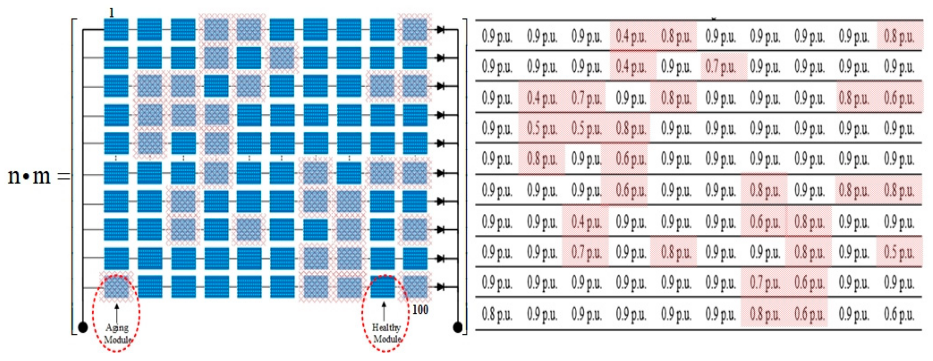
3. The Offline Reconfiguration Strategy without Replacing Extremely Aged Modules
4. Photovoltaic Array Reconfiguration Optimization Scheme
4.1. Reconfiguration Based on Gene Evolution Algorithm (GEA)
- Creation of the fitness function as a normalized quantity: the suggested fitness function is expressed by Equation (2), as follows in Figure 7 and the GEA is intended to increase the pvi value to the maximum;
- Parametric design underpinned by three conditions, namely, a population size of 300, a chromosome length of n*m, and number of evolution times of 3000;
- Decimal-based encoding approach: direct encoding with the PV module number; thus, chromosome expression can take the form of a sequence ;
- Fitness assessment of all chromosomes in the population: after chromosome conversion into a two-dimensional array (n*m), pvi calculation is undertaken based on the formulated fitness function;
- Appraisal to achieve iterations or optimization aim: steps 6–8 can be bypassed only if appraisal succeeds;
- Choice of parents for the future generation: this involves sorting the fitness from large to small to choose the surviving chromosomes, followed by arbitrary selection of individuals surviving despite small fitness;
- Parental chromosome crossbreeding: this issue is challenging due to the cross-over approach; the order cross-over technique is employed in the case of the direct use of the point cross, which will cause problems of PV-model duplication and omission in the offspring chromosomes; two hybridization points are chosen arbitrarily between the parents by the sequential hybridization algorithm, with subsequent exchange of hybridization segments and the relative locations of the parental models help to establish the other locations; for example, the chromosome can be given as the sequence .
- ❖
- Parent one =
- ❖
- Parent two = .
- ❖
- Parent one’ =
- ❖
- Parent two’= .
- ❖
- Parent one’ = , from the second crossing point in turn.
- ❖
- Parent two’ = .
- Chromosomal mutation: this helps to both diversify the population and to ensure universal optimization; the particular rate of mutation for the chosen mutant individual is the basis for the arbitrary selection of three integers that meet the condition 1 < u < v < w < n*m and the genes between v and u including u and v, with paragraph insertion after w; the fourth step is subsequently undertaken;
- Optimal output chromosome: comparative analysis between every configuration satisfying every step and the initial configuration is shown in Figure 8.
4.2. Cost Analysis of Rearrangements for PV Array
- PVpre is the PV array output power before arrangements
- PVpost is the output power after arrangements
- Ae is the additional electricity
- Hw is the average hourly wage of the manpower (60 min)
- Ep is the electricity price
- Ns is the number of swaps/replace
- Ts is the time per swap/replace
- Cper is the cost per swap/replace
- C sawp is the cost of swaps
- C replace is the cost of replace
- Wt Cost is the cost per watt peak (cents/Wp)
- Ss is the size per module (Wp)
- USD is United States Dollar ($)
5. Case Studies and Simulation Results
5.1. Case 1 (Arrange Aging Modules of 10 × 10 PV Array)
5.1.1. Scenario One (Initial–Final Rates Return of Electricity Revenue)
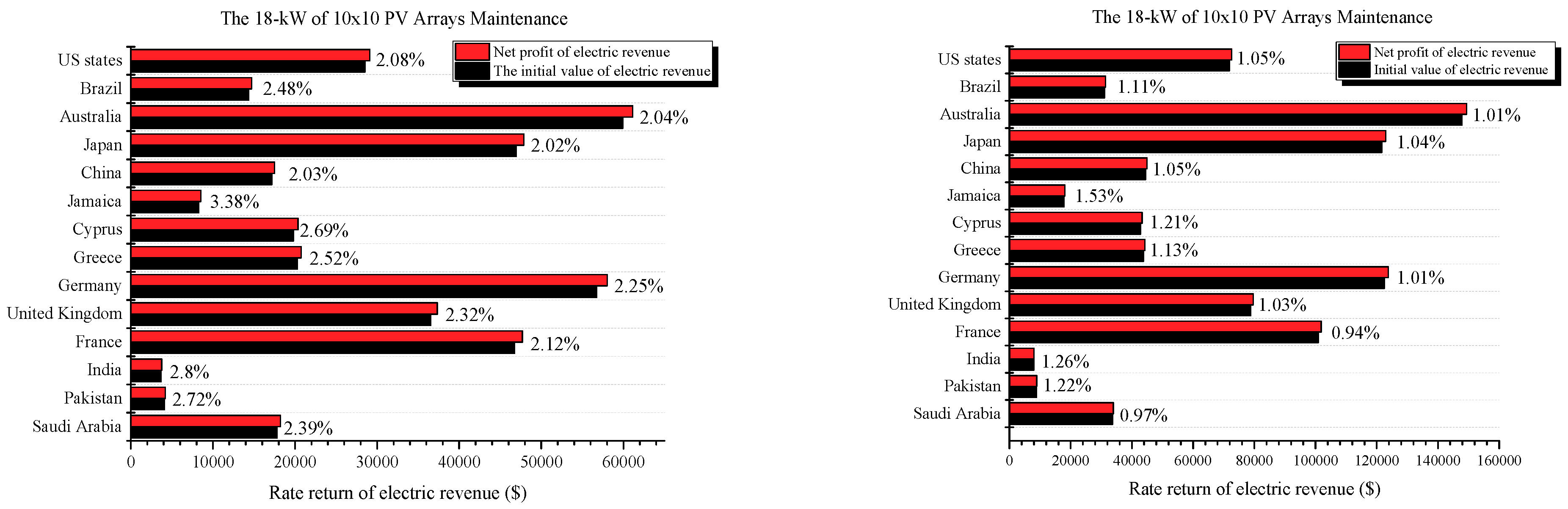
5.1.2. Scenario Two (Net Profits of Additional Electric Revenue)
5.2. Case 2 (Combine Swap/Replace Aging Modules of 10 × 10 PV Array)
5.2.1. Scenario One (Initial-Final Rates Return of Electricity Revenue)
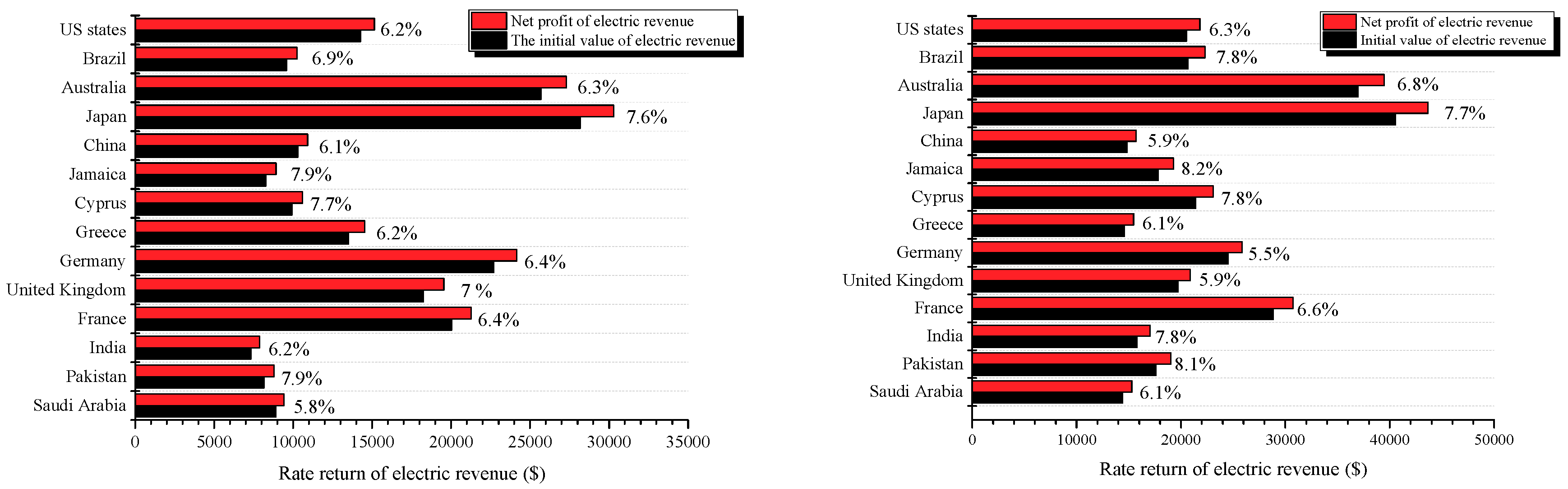
5.2.2. Scenario Two (Net Profits of Additional Electric Revenue)
6. Analysis Outcomes
7. Conclusions
Author Contributions
Funding
Institutional Review Board Statement
Informed Consent Statement
Data Availability Statement
Acknowledgments
Conflicts of Interest
References
- Dida, M.; Boughali, S.; Bechki, D.; Bouguettaia, H. Output power loss of crystalline silicon photovoltaic modules due to dust accumulation in Saharan environment. Renew. Sustain. Energy Rev. 2020, 124, 109787. [Google Scholar] [CrossRef]
- Hu, Y.; Zhang, J.; Wu, J.; Cao, W.; Tian, G.Y.; Kirtley, J.L. Efficiency Improvement of Nonuniformly Aged PV Arrays. IEEE Trans. Power Electron. 2017, 32, 1124–1137. [Google Scholar] [CrossRef]
- Alkahtani, M.; Hu, Y.; Wu, Z.; Kuka, C.S.; Alhammad, M.S.; Zhang, C. Gene Evaluation Algorithm for Reconfiguration of Medium and Large Size Photovoltaic Arrays Exhibiting Non-Uniform Aging. Energies 2020, 13, 1921. [Google Scholar] [CrossRef]
- Osterwald, C.R.; Anderberg, A.; Rummel, S.; Ottoson, L. Degradation analysis of weathered crystalline-silicon PV modules. In Proceedings of the Conference Record of the Twenty-Ninth IEEE Photovoltaic Specialists Conference, New Orleans, LA, USA, 19–24 May 2002; pp. 1392–1395. [Google Scholar]
- Ndiaye, A.; Kébé, C.M.F.; Ndiaye, P.A.; Charki, A.; Kobi, A.; Sambou, V. A Novel Method for Investigating Photovoltaic Module Degradation. Energy Procedia 2013, 36, 1222–1231. [Google Scholar] [CrossRef]
- Munoz, M.A.; Alonso-García, M.C.; Vela, N.; Chenlo, F. Early degradation of silicon PV modules and guaranty conditions. Solar Energy 2011, 85, 2264–2274. [Google Scholar] [CrossRef]
- Hu, Y.; Zhang, J.; Li, P.; Yu, D.; Jiang, L. Non-Uniform Aged Modules Reconfiguration for Large-Scale PV Array. IEEE Trans. Device Mater. Reliab. 2017, 17, 560–569. [Google Scholar] [CrossRef]
- Orozco-Gutierrez, M.L.; Spagnuolo, G.; Ramirez-Scarpetta, J.M.; Petrone, G.; Ramos-Paja, C.A. Optimized Configuration of Mismatched Photovoltaic Arrays. IEEE J. Photovol. 2016, 6, 1210–1220. [Google Scholar] [CrossRef]
- Velasco-Quesada, G.; Guinjoan-Gispert, F.; Pique-Lopez, R.; Roman-Lumbreras, M.; Conesa-Roca, A. Electrical PV Array Reconfiguration Strategy for Energy Extraction Improvement in Grid-Connected PV Systems. IEEE Trans. Ind. Electron. 2009, 56, 4319–4331. [Google Scholar] [CrossRef]
- Tanesab, J.; Parlevliet, D.; Whale, J.; Urmee, T. Dust Effect and its Economic Analysis on PV Modules Deployed in a Temperate Climate Zone. Energy Procedia 2016, 100, 65–68. [Google Scholar] [CrossRef]
- Alahmad, M.; Chaaban, M.A.; Lau, S.k.; Shi, J.; Neal, J. An adaptive utility interactive photovoltaic system based on a flexible switch matrix to optimize performance in real-time. Solar Energy 2012, 86, 951–963. [Google Scholar] [CrossRef]
- Schultz-Wittmann, O.; Glunz, S.; Willeke, G. Multicrystalline Silicon Solar Cells Exceeding 20% Efficiency. Prog. Photovol. Res. Appl. 2004, 12, 553–558. [Google Scholar] [CrossRef]
- Zhang, H.; Lu, Y.; Han, W.; Zhu, J.; Zhang, Y.; Huang, W. Solar energy conversion and utilization: Towards the emerging photo-electrochemical devices based on perovskite photovoltaics. Chem. Eng. J. 2020, 393, 124766. [Google Scholar] [CrossRef]
- Li, W.; Li, W.; Xiang, X.; Hu, Y.; He, X. High Step-Up Interleaved Converter With Built-In Transformer Voltage Multiplier Cells for Sustainable Energy Applications. IEEE Trans. Power Electr. 2014, 29, 2829–2836. [Google Scholar] [CrossRef]
- Hu, Y.; Deng, Y.; Liu, Q.; He, X. Asymmetry Three-Level Gird-Connected Current Hysteresis Control With Varying Bus Voltage and Virtual Oversample Method. IEEE Trans. Power Electr. 2014, 29, 3214–3222. [Google Scholar] [CrossRef]
- Rabaia, M.K.H.; Abdelkareem, M.A.; Sayed, E.T.; Elsaid, K.; Chae, K.-J.; Wilberforce, T.; Olabi, A.G. Environmental impacts of solar energy systems: A review. Sci. Total Environ. 2021, 754, 141989. [Google Scholar] [CrossRef] [PubMed]
- Alkahtani, M.; Wu, Z.; Kuka, C.S.; Alahammad, M.S.; Ni, K. A Novel PV Array Reconfiguration Algorithm Approach to Optimising Power Generation across Non-uniformly Aged PV Arrays by merely Repositioning. J. Multidisc. Sci. J. 2020, 3, 32–53. [Google Scholar] [CrossRef]
- Soliman, M.A.; Hasanien, H.M.; Alkuhayli, A. Marine Predators Algorithm for Parameters Identification of Triple-Diode Photovoltaic Models. IEEE Access 2020, 8, 155832–155842. [Google Scholar] [CrossRef]
- Takashima, T.; Yamaguchi, J.; Otani, K.; Oozeki, T.; Kato, K.; Ishida, M. Experimental studies of fault location in PV module strings. Solar Energy Mater. Solar Cells 2009, 93, 1079–1082. [Google Scholar] [CrossRef]
- Meyer, E.L.; Dyk, E.E.v. Assessing the reliability and degradation of photovoltaic module performance parameters. IEEE Trans. Reliab. 2004, 53, 83–92. [Google Scholar] [CrossRef]
- Hu, Y.; Cao, W.; Wu, J.; Ji, B.; Holliday, D. Thermography-Based Virtual MPPT Scheme for Improving PV Energy Efficiency Under Partial Shading Conditions. IEEE Trans. Power Electr. 2014, 29, 5667–5672. [Google Scholar] [CrossRef]
- Kumar, R.A.; Suresh, M.S.; Nagaraju, J. Measurement of AC parameters of gallium arsenide (GaAs/Ge) solar cell by impedance spectroscopy. IEEE Trans. Electron Dev. 2001, 48, 2177–2179. [Google Scholar] [CrossRef]
- Mattei, M.; Notton, G.; Cristofari, C.; Muselli, M.; Poggi, P. Calculation of the polycrystalline PV module temperature using a simple method of energy balance. Renew. Energy 2006, 31, 553–567. [Google Scholar] [CrossRef]
- Chouder, A.; Silvestre, S. Automatic supervision and fault detection of PV systems based on power losses analysis. Energy Convers. Manag. 2010, 51, 1929–1937. [Google Scholar] [CrossRef]
- Silvestre, S.; Chouder, A.; Karatepe, E. Automatic fault detection in grid connected PV systems. Solar Energy 2013, 94, 119–127. [Google Scholar] [CrossRef]
- Nguyen, D.; Lehman, B. An Adaptive Solar Photovoltaic Array Using Model-Based Reconfiguration Algorithm. IEEE Trans. Ind. Electron. 2008, 55, 2644–2654. [Google Scholar] [CrossRef]
- Storey, J.P.; Wilson, P.R.; Bagnall, D. Improved Optimization Strategy for Irradiance Equalization in Dynamic Photovoltaic Arrays. IEEE Trans. Power Electr. 2013, 28, 2946–2956. [Google Scholar] [CrossRef]
- Storey, J.; Wilson, P.R.; Bagnall, D. The Optimized-String Dynamic Photovoltaic Array. IEEE Trans. Power Electr. 2014, 29, 1768–1776. [Google Scholar] [CrossRef]
- Cristaldi, L.; Faifer, M.; Rossi, M.; Toscani, S.; Catelani, M.; Ciani, L.; Lazzaroni, M. Simplified method for evaluating the effects of dust and aging on photovoltaic panels. Measurement 2014, 54, 207–214. [Google Scholar] [CrossRef]
- Wu, Z.; Zhang, C.; Alkahtani, M.; Hu, Y.; Zhang, J. Cost Effective Offline Reconfiguration for Large-Scale Non-Uniformly Aging Photovoltaic Arrays Efficiency Enhancement. IEEE Access 2020, 8, 80572–80581. [Google Scholar] [CrossRef]
- Global Petrp Prices. Electricity Prices around the World. Available online: https://www.globalpetrolprices.com/electricity_prices/ (accessed on 20 November 2020).
- Salary Expert. Electrician Salary. Available online: https://www.salaryexpert.com/salary/job/electrician/ (accessed on 25 November 2020).
- Lazard. Levelized Cost of Energy and Levelized Cost of Storage–2020. Available online: https://www.lazard.com/perspective/levelized-cost-of-energy-and-levelized-cost-of-storage-2020/ (accessed on 25 November 2020).
- IRENA. Renewable Power Generation Costs-2019. Available online: https://www.irena.org/publications/2020/Jun/Renewable-Power-Costs-in-2019 (accessed on 25 November 2020).
- Djordjevic, S.; Parlevliet, D.; Jennings, P. Detectable faults on recently installed solar modules in Western Australia. Renew. Energy 2014, 67, 215–221. [Google Scholar] [CrossRef]
- Wang, Z.; Zhou, N.; Gong, L.; Jiang, M. Quantitative estimation of mismatch losses in photovoltaic arrays under partial shading conditions. Optik 2020, 203, 163950. [Google Scholar] [CrossRef]
- Nobile, G.; Vasta, E.; Cacciato, M.; Scarcella, G.; Scelba, G.; Stefano, A.G.F.D.; Leotta, G.; Pugliatti, P.M.; Bizzarri, F. Study on mismatch losses in large PV plants: Data analysis of a case study and modeling approach. In Proceedings of the 2020 International Symposium on Power Electronics, Electrical Drives, Automation and Motion (SPEEDAM), Sorrento, Italy, 24–26 June 2020; pp. 858–864. [Google Scholar]


| Parameter | Value | Units | Symbols |
|---|---|---|---|
| Open-circuit voltage | 21.10 | V | VOC |
| Short-circuit current | 3.8 | A | ISC |
| MPP power | 60 | W | Pmpp |
| MPP current | 3.5 | A | Impp |
| MPP voltage | 17.10 | V | Vmpp |
| Cell temperature | 25 | °C | T |
| Pre-Arrangement | |||||||||
|---|---|---|---|---|---|---|---|---|---|
| 0.9 p.u. | 0.9 p.u. | 0.9 p.u. | 0.4 p.u. | 0.9 p.u. | 0.9 p.u. | 0.6 p.u. | 0.9 p.u. | 0.8 p.u. | 0.9 p.u. |
| 0.6 p.u. | 0.9 p.u. | 0.5 p.u. | 0.9 p.u. | 0.9 p.u. | 0.8 p.u. | 0.9 p.u. | 0.9 p.u. | 0.6 p.u. | 0.8 p.u. |
| 0.9 p.u. | 0.8 p.u. | 0.9 p.u. | 0.9 p.u. | 0.9 p.u. | 0.9 p.u. | 0.9 p.u. | 0.9 p.u. | 0.8 p.u. | 0.8 p.u. |
| 0.9 p.u. | 0.9 p.u. | 0.8 p.u. | 0.9 p.u. | 0.9 p.u. | 0.9 p.u. | 0.7 p.u. | 0.9 p.u. | 0.9 p.u. | 0.9 p.u. |
| 0.5 p.u. | 0.6 p.u. | 0.9 p.u. | 0.9 p.u. | 0.9 p.u. | 0.9 p.u. | 0.9 p.u. | 0.7 p.u. | 0.9 p.u. | 0.9 p.u. |
| 0.9 p.u. | 0.9 p.u. | 0.9 p.u. | 0.4 p.u. | 0.9 p.u. | 0.9 p.u. | 0.9 p.u. | 0.8 p.u. | 0.5 p.u. | 0.9 p.u. |
| 0.6 p.u. | 0.9 p.u. | 0.9 p.u. | 0.9 p.u. | 0.9 p.u. | 0.8 p.u. | 0.9 p.u. | 0.9 p.u. | 0.6 p.u. | 0.8 p.u. |
| 0.9 p.u. | 0.8 p.u. | 0.9 p.u. | 0.9 p.u. | 0.9 p.u. | 0.9 p.u. | 0.9 p.u. | 0.9 p.u. | 0.8 p.u. | 0.8 p.u. |
| 0.9 p.u. | 0.9 p.u. | 0.8 p.u. | 0.9 p.u. | 0.9 p.u. | 0.9 p.u. | 0.7 p.u. | 0.9 p.u. | 0.9 p.u. | 0.9 p.u. |
| 0.4 p.u. | 0.6 p.u. | 0.9 p.u. | 0.9 p.u. | 0.9 p.u. | 0.9 p.u. | 0.9 p.u. | 0.7 p.u. | 0.9 p.u. | 0.9 p.u. |
| Post-Arrangement | |||||||||
|---|---|---|---|---|---|---|---|---|---|
| 0.9 p.u. | 0.9 p.u. | 0.9 p.u. | 0.4 p.u. | 0.8 p.u. | 0.9 p.u. | 0.9 p.u. | 0.9 p.u. | 0.9 p.u. | 0.8 p.u. |
| 0.9 p.u. | 0.9 p.u. | 0.9 p.u. | 0.4 p.u. | 0.9 p.u. | 0.7 p.u. | 0.9 p.u. | 0.9 p.u. | 0.9 p.u. | 0.9 p.u. |
| 0.9 p.u. | 0.4 p.u. | 0.7 p.u. | 0.9 p.u. | 0.8 p.u. | 0.9 p.u. | 0.9 p.u. | 0.9 p.u. | 0.8 p.u. | 0.6 p.u. |
| 0.9 p.u. | 0.5 p.u. | 0.5 p.u. | 0.8 p.u. | 0.9 p.u. | 0.9 p.u. | 0.9 p.u. | 0.9 p.u. | 0.9 p.u. | 0.9 p.u. |
| 0.9 p.u. | 0.8 p.u. | 0.9 p.u. | 0.6 p.u. | 0.9 p.u. | 0.9 p.u. | 0.9 p.u. | 0.9 p.u. | 0.9 p.u. | 0.9 p.u. |
| 0.9 p.u. | 0.9 p.u. | 0.9 p.u. | 0.6 p.u. | 0.9 p.u. | 0.9 p.u. | 0.8 p.u. | 0.9 p.u. | 0.8 p.u. | 0.8 p.u. |
| 0.9 p.u. | 0.9 p.u. | 0.4 p.u. | 0.9 p.u. | 0.9 p.u. | 0.9 p.u. | 0.6 p.u. | 0.8 p.u. | 0.9 p.u. | 0.9 p.u. |
| 0.9 p.u. | 0.9 p.u. | 0.7 p.u. | 0.9 p.u. | 0.8 p.u. | 0.9 p.u. | 0.9 p.u. | 0.8 p.u. | 0.9 p.u. | 0.5 p.u. |
| 0.9 p.u. | 0.9 p.u. | 0.9 p.u. | 0.9 p.u. | 0.9 p.u. | 0.9 p.u. | 0.7 p.u. | 0.6 p.u. | 0.9 p.u. | 0.9 p.u. |
| 0.8 p.u. | 0.9 p.u. | 0.9 p.u. | 0.9 p.u. | 0.9 p.u. | 0.9 p.u. | 0.8 p.u. | 0.6 p.u. | 0.9 p.u. | 0.6 p.u. |
| Country | Electricity Prices $/kWh | Hourly Wage $/hr | Cost Per Swap $/time | Cost Per Replace $/time |
|---|---|---|---|---|
| Saudi Arabia | 0.059 | 7.98 | 5.98 | 3.99 |
| Pakistan | 0.108 | 1.42 | 1.07 | 0.71 |
| India | 0.097 | 1.19 | 0.89 | 0.60 |
| France | 0.177 | 24.87 | 18.65 | 12.44 |
| United Kingdom | 0.242 | 17.2 | 12.9 | 8.60 |
| Germany | 0.301 | 27.91 | 20.93 | 13.96 |
| Greece | 0.179 | 8.28 | 6.21 | 4.14 |
| Cyprus | 0.263 | 7.11 | 5.21 | 3.56 |
| Jamaica | 0.219 | 1.24 | 0.93 | 0.62 |
| China | 0.091 | 9.57 | 7.17 | 4.79 |
| Japan | 0.249 | 26.33 | 19.74 | 13.17 |
| Australia | 0.227 | 33.35 | 25.02 | 16.68 |
| Brazil | 0.127 | 6.05 | 4.54 | 3.03 |
| US states | 0.126 | 15.47 | 11.8 | 7.78 |
| Pre-Arrangement | |||||||||
| 0.9 p.u. | 0.9 p.u. | 0.9 p.u. | 0.4 p.u. | 0.9 p.u. | 0.9 p.u. | 0.6 p.u. | 0.9 p.u. | 0.8 p.u. | 0.9 p.u. |
| 0.6 p.u. | 0.9 p.u. | 0.5 p.u. | 0.9 p.u. | 0.9 p.u. | 0.8 p.u. | 0.9 p.u. | 0.9 p.u. | 0.6 p.u. | 0.8 p.u. |
| 0.9 p.u. | 0.8 p.u. | 0.9 p.u. | 0.9 p.u. | 0.9 p.u. | 0.9 p.u. | 0.9 p.u. | 0.9 p.u. | 0.8 p.u. | 0.8 p.u. |
| 0.9 p.u. | 0.9 p.u. | 0.8 p.u. | 0.9 p.u. | 0.9 p.u. | 0.9 p.u. | 0.7 p.u. | 0.9 p.u. | 0.9 p.u. | 0.9 p.u. |
| 0.5 p.u. | 0.6 p.u. | 0.9 p.u. | 0.9 p.u. | 0.9 p.u. | 0.9 p.u. | 0.9 p.u. | 0.7 p.u. | 0.9 p.u. | 0.9 p.u. |
| 0.9 p.u. | 0.9 p.u. | 0.9 p.u. | 0.4 p.u. | 0.9 p.u. | 0.9 p.u. | 0.9 p.u. | 0.8 p.u. | 0.5 p.u. | 0.9 p.u. |
| 0.6 p.u. | 0.9 p.u. | 0.9 p.u. | 0.9 p.u. | 0.9 p.u. | 0.8 p.u. | 0.9 p.u. | 0.9 p.u. | 0.6 p.u. | 0.8 p.u. |
| 0.9 p.u. | 0.8 p.u. | 0.9 p.u. | 0.9 p.u. | 0.9 p.u. | 0.9 p.u. | 0.9 p.u. | 0.9 p.u. | 0.8 p.u. | 0.8 p.u. |
| 0.9 p.u. | 0.9 p.u. | 0.8 p.u. | 0.9 p.u. | 0.9 p.u. | 0.9 p.u. | 0.7 p.u. | 0.9 p.u. | 0.9 p.u. | 0.9 p.u. |
| 0.4 p.u. | 0.6 p.u. | 0.9 p.u. | 0.9 p.u. | 0.9 p.u. | 0.9 p.u. | 0.9 p.u. | 0.7 p.u. | 0.9 p.u. | 0.9 p.u. |
| Post-Arrangement | |||||||||
| 0.9 p.u. | 0.9 p.u. | 0.9 p.u. | 0.4 p.u. | 0.8 p.u. | 0.9 p.u. | 0.9 p.u. | 0.9 p.u. | 0.9 p.u. | 0.8 p.u. |
| 0.9 p.u. | 0.9 p.u. | 0.9 p.u. | 0.4 p.u. | 0.9 p.u. | 0.7 p.u. | 0.9 p.u. | 0.9 p.u. | 0.9 p.u. | 0.9 p.u. |
| 0.9 p.u. | 0.9 p.u. | 0.7 p.u. | 0.9 p.u. | 0.8 p.u. | 0.9 p.u. | 0.9 p.u. | 0.9 p.u. | 0.8 p.u. | 0.6 p.u. |
| 0.9 p.u. | 0.5 p.u. | 0.5 p.u. | 0.8 p.u. | 0.9 p.u. | 0.9 p.u. | 0.9 p.u. | 0.9 p.u. | 0.9 p.u. | 0.9 p.u. |
| 0.9 p.u. | 0.8 p.u. | 0.9 p.u. | 0.6 p.u. | 0.9 p.u. | 0.9 p.u. | 0.9 p.u. | 0.9 p.u. | 0.9 p.u. | 0.9 p.u. |
| 0.9 p.u. | 0.9 p.u. | 0.9 p.u. | 0.6 p.u. | 0.9 p.u. | 0.9 p.u. | 0.8 p.u. | 0.9 p.u. | 0.8 p.u. | 0.8 p.u. |
| 0.9 p.u. | 0.9 p.u. | 0.4 p.u. | 0.9 p.u. | 0.9 p.u. | 0.9 p.u. | 0.6 p.u. | 0.8 p.u. | 0.9 p.u. | 0.9 p.u. |
| 0.9 p.u. | 0.9 p.u. | 0.7 p.u. | 0.9 p.u. | 0.8 p.u. | 0.9 p.u. | 0.9 p.u. | 0.8 p.u. | 0.9 p.u. | 0.5 p.u. |
| 0.9 p.u. | 0.9 p.u. | 0.9 p.u. | 0.9 p.u. | 0.9 p.u. | 0.9 p.u. | 0.7 p.u. | 0.6 p.u. | 0.9 p.u. | 0.9 p.u. |
| 0.8 p.u. | 0.9 p.u. | 0.9 p.u. | 0.9 p.u. | 0.9 p.u. | 0.9 p.u. | 0.8 p.u. | 0.6 p.u. | 0.9 p.u. | 0.6 p.u. |
| Country | Initial Rate Return of Electric Revenue 18-kW ($) | Final Rate Return of Electric Revenue 18-kW ($) | Initial Rate Return of Electric Revenue 43-kW ($) | Final Rate Return of Electric Revenue 43-kW ($) |
|---|---|---|---|---|
| Saudi Arabia | 17,795.83 | 18,484.95 | 33,625.78 | 34,216.7 |
| Pakistan | 4071.93 | 4229.61 | 8793.18 | 8947.71 |
| India | 3657.19 | 3798.81 | 7897.58 | 8036.37 |
| France | 46,714.07 | 48,523.01 | 100,877.35 | 102,650.11 |
| United Kingdom | 36,496.54 | 37,909.82 | 78,812.97 | 80,197.99 |
| Germany | 56,743.08 | 58,940.38 | 122,534.63 | 124,687.99 |
| Greece | 20,246.53 | 21,030.55 | 43,721.66 | 44,490.01 |
| Cyprus | 19,831.8 | 20,599.76 | 42,826.06 | 43,578.66 |
| Jamaica | 8256.97 | 8576.71 | 17,830.62 | 18,143.97 |
| China | 17,154.88 | 17,819.18 | 44,454.42 | 45,235.64 |
| Japan | 46,940.28 | 48,757.98 | 121,639.03 | 12,3776.65 |
| Australia | 59,910.13 | 62,230.07 | 147,855.74 | 150,454.07 |
| Brazil | 14,364.86 | 14,921.12 | 31,020.4 | 31,565.53 |
| US states | 28,503.5 | 29,607.26 | 71,810.99 | 73,072.96 |
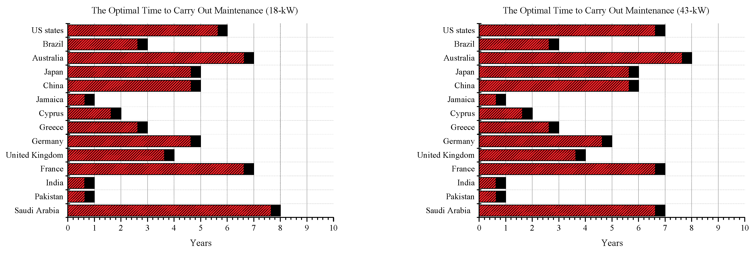
| Country | Cost of Swapping 44 Modules $/time | Best Cost-Effective Maintenance Period Time | Additional Electric Revenue 18-kW ($) | Cost of Swapping 44 Modules $/time | Best Cost-Effective Maintenance Period Time | Additional Electric Revenue 43-kW ($) |
|---|---|---|---|---|---|---|
| Saudi Arabia | 263.34 | 8 | 607.9 | 263.34 | 7 | 327.58 |
| Pakistan | 46.86 | 1 | 110.82 | 46.86 | 1 | 107.67 |
| India | 39.27 | 1 | 102.35 | 39.27 | 1 | 99.52 |
| France | 820.71 | 7 | 988.23 | 820.71 | 7 | 952.05 |
| United Kingdom | 567.60 | 4 | 845.68 | 567.60 | 4 | 817.41 |
| Germany | 921.03 | 5 | 1276.27 | 921.03 | 5 | 1232.32 |
| Greece | 273.24 | 3 | 510.78 | 273.24 | 3 | 495.10 |
| Cyprus | 234.63 | 2 | 533.33 | 234.63 | 2 | 517.97 |
| Jamaica | 40.92 | 1 | 278.82 | 40.92 | 1 | 272.43 |
| China | 315.81 | 5 | 348.49 | 315.81 | 6 | 465.41 |
| Japan | 868.89 | 5 | 948.81 | 868.89 | 6 | 1268.73 |
| Australia | 1100.55 | 7 | 1219.39 | 1100.55 | 8 | 1497.78 |
| Brazil | 199.65 | 3 | 356.61 | 199.65 | 3 | 345.48 |
| US states | 510.51 | 6 | 593.25 | 510.51 | 7 | 751.46 |
| Country | The Initial Value of Electric Revenue without Considering Labor Cost 18-kW ($) | Net Profit of Final Value Electric Revenue by Considering Labor Cost 18-kW ($) | The Initial Value of Electric Revenue without Considering Labor Cost 43-kW ($) | Net Profit of Final Value Electric Revenue by Considering Labor Cost 43-kW ($) |
|---|---|---|---|---|
| Saudi Arabia | 17,795.83 | 18,221.61 | 33,625.78 | 33,953.36 |
| Pakistan | 4071.93 | 4182.75 | 8793.18 | 8900.85 |
| India | 3657.19 | 3759.54 | 7897.58 | 7997.1 |
| France | 46,714.07 | 47,702.3 | 100,877.35 | 101,829.4 |
| United Kingdom | 36,496.54 | 37,342.22 | 78,812.97 | 79,630.39 |
| Germany | 56,743.08 | 58,019.35 | 122,534.63 | 123,766.96 |
| Greece | 20,246.53 | 20,757.31 | 43,721.66 | 44,216.77 |
| Cyprus | 19,831.8 | 20,365.13 | 42,826.06 | 43,344.03 |
| Jamaica | 8256.97 | 8535.79 | 17,830.62 | 18,103.05 |
| China | 17,154.88 | 17,503.37 | 44,454.42 | 44,919.83 |
| Japan | 46,940.28 | 47,889.09 | 121,639.03 | 122,907.76 |
| Australia | 59,910.13 | 61,129.52 | 147,855.74 | 149,353.52 |
| Brazil | 14,364.86 | 14,721.47 | 31,020.4 | 31,365.88 |
| US states | 28,503.5 | 29,096.75 | 71,810.99 | 72,562.45 |
| Parameters Input | 10 × 10 PV Array 18 kW | 10 × 10 PV Array 43 kW | Unit |
|---|---|---|---|
| Number of Replace | 6 | 6 | PV module |
| Number of Swap | 38 | 38 | PV module |
| Time per replace | 30 | 30 | Minute |
| Time per swap | 45 | 45 | Minute |
| Cost per panel | 40 | 70 | USD |
| Cost per watt peak | 0.22 | 0.36 | Cents/Wp |
| Size per module | 180 | 430 | Wp |
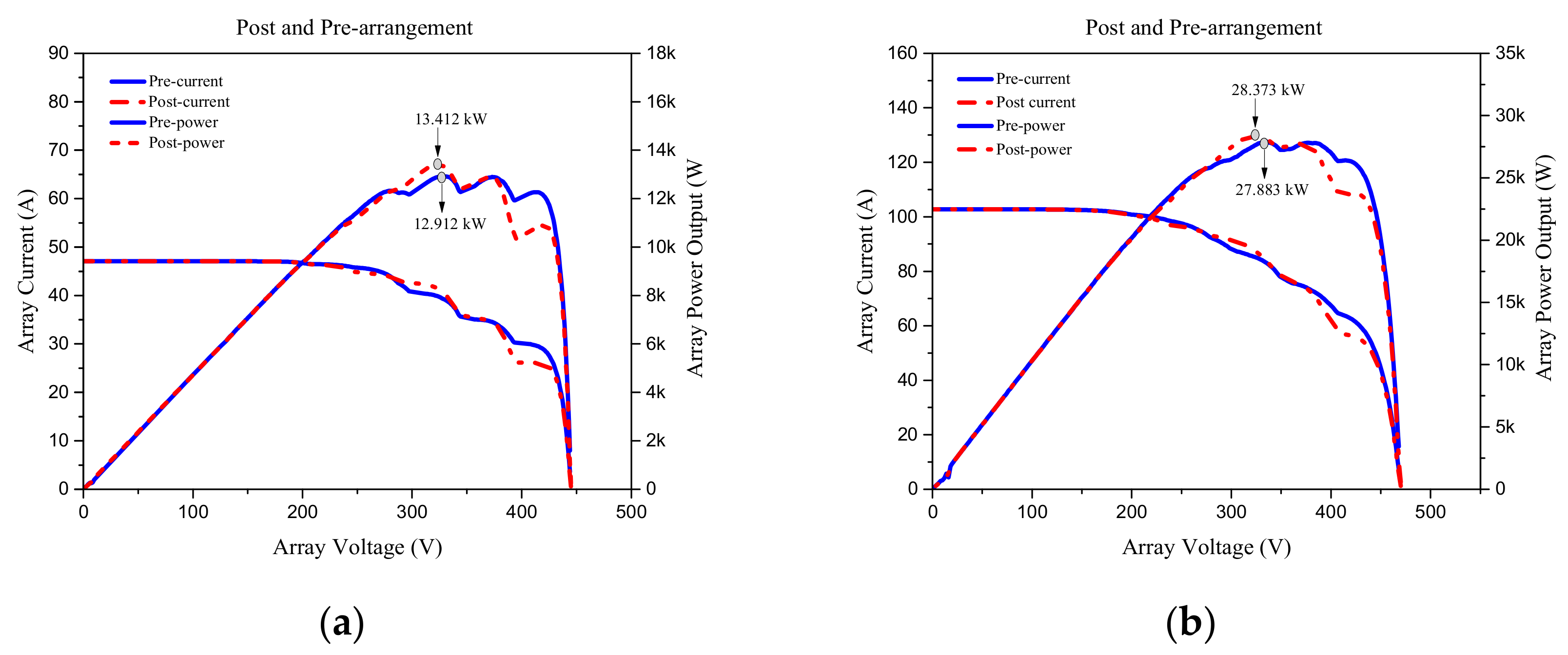
| Initial Output | 12.912 | 27.883 | kW |
| Final Output | 15.957 | 33.990 | kW |
| Difference | 3.045 | 6.108 | kW |
| Number of Replace | 6 | 6 | PV module |
| Number of Swap | 38 | 38 | PV module |
| Pre-Arrangement | |||||||||
| 0.9 p.u. | 0.9 p.u. | 0.9 p.u. | 0.4 p.u. | 0.9 p.u. | 0.9 p.u. | 0.6 p.u. | 0.9 p.u. | 0.8 p.u. | 0.9 p.u. |
| 0.6 p.u. | 0.9 p.u. | 0.5 p.u. | 0.9 p.u. | 0.9 p.u. | 0.8 p.u. | 0.9 p.u. | 0.9 p.u. | 0.6 p.u. | 0.8 p.u. |
| 0.9 p.u. | 0.8 p.u. | 0.9 p.u. | 0.9 p.u. | 0.9 p.u. | 0.9 p.u. | 0.9 p.u. | 0.9 p.u. | 0.8 p.u. | 0.8 p.u. |
| 0.9 p.u. | 0.9 p.u. | 0.8 p.u. | 0.9 p.u. | 0.9 p.u. | 0.9 p.u. | 0.7 p.u. | 0.9 p.u. | 0.9 p.u. | 0.9 p.u. |
| 0.5 p.u. | 0.6 p.u. | 0.9 p.u. | 0.9 p.u. | 0.9 p.u. | 0.9 p.u. | 0.9 p.u. | 0.7 p.u. | 0.9 p.u. | 0.9 p.u. |
| 0.9 p.u. | 0.9 p.u. | 0.9 p.u. | 0.4 p.u. | 0.9 p.u. | 0.9 p.u. | 0.9 p.u. | 0.8 p.u. | 0.5 p.u. | 0.9 p.u. |
| 0.6 p.u. | 0.9 p.u. | 0.9 p.u. | 0.9 p.u. | 0.9 p.u. | 0.8 p.u. | 0.9 p.u. | 0.9 p.u. | 0.6 p.u. | 0.8 p.u. |
| 0.9 p.u. | 0.8 p.u. | 0.9 p.u. | 0.9 p.u. | 0.9 p.u. | 0.9 p.u. | 0.9 p.u. | 0.9 p.u. | 0.8 p.u. | 0.8 p.u. |
| 0.9 p.u. | 0.9 p.u. | 0.8 p.u. | 0.9 p.u. | 0.9 p.u. | 0.9 p.u. | 0.7 p.u. | 0.9 p.u. | 0.9 p.u. | 0.9 p.u. |
| 0.4 p.u. | 0.6 p.u. | 0.9 p.u. | 0.9 p.u. | 0.9 p.u. | 0.9 p.u. | 0.9 p.u. | 0.7 p.u. | 0.9 p.u. | 0.9 p.u. |
| Post-Arrangement | |||||||||
| 0.9 p.u. | 0.9 p.u. | 0.9 p.u. | 1 p.u. | 0.8 p.u. | 0.9 p.u. | 0.9 p.u. | 0.9 p.u. | 0.9 p.u. | 0.8 p.u. |
| 0.9 p.u. | 0.9 p.u. | 0.9 p.u. | 1 p.u. | 0.9 p.u. | 0.7 p.u. | 0.9 p.u. | 0.9 p.u. | 0.9 p.u. | 0.9 p.u. |
| 0.9 p.u. | 0.9 p.u. | 0.7 p.u. | 0.9 p.u. | 0.8 p.u. | 0.9 p.u. | 0.9 p.u. | 0.9 p.u. | 0.8 p.u. | 0.6 p.u. |
| 0.9 p.u. | 1 p.u. | 1 p.u. | 0.8 p.u. | 0.9 p.u. | 0.9 p.u. | 0.9 p.u. | 0.9 p.u. | 0.9 p.u. | 0.9 p.u. |
| 0.9 p.u. | 0.8 p.u. | 0.9 p.u. | 0.6 p.u. | 0.9 p.u. | 0.9 p.u. | 0.9 p.u. | 0.9 p.u. | 0.9 p.u. | 0.9 p.u. |
| 0.9 p.u. | 0.9 p.u. | 0.9 p.u. | 0.6 p.u. | 0.9 p.u. | 0.9 p.u. | 0.8 p.u. | 0.9 p.u. | 0.8 p.u. | 0.8 p.u. |
| 0.9 p.u. | 0.9 p.u. | 1 p.u. | 0.9 p.u. | 0.9 p.u. | 0.9 p.u. | 0.6 p.u. | 0.8 p.u. | 0.9 p.u. | 0.9 p.u. |
| 0.9 p.u. | 0.9 p.u. | 0.7 p.u. | 0.9 p.u. | 0.8 p.u. | 0.9 p.u. | 0.9 p.u. | 0.8 p.u. | 0.9 p.u. | 1 p.u. |
| 0.9 p.u. | 0.9 p.u. | 0.9 p.u. | 0.9 p.u. | 0.9 p.u. | 0.9 p.u. | 0.7 p.u. | 0.6 p.u. | 0.9 p.u. | 0.9 p.u. |
| 0.8 p.u. | 0.9 p.u. | 0.9 p.u. | 0.9 p.u. | 0.9 p.u. | 0.9 p.u. | 0.8 p.u. | 0.6 p.u. | 0.9 p.u. | 0.6 p.u. |
| Country | Initial Rate Return of Electric Revenue 18-kW ($) | Final Rate Return of Electric Revenue 18-kW ($) | Initial Rate Return of Electric Revenue 43-kW ($) | Final Rate Return of Electric Revenue 43-kW ($) |
|---|---|---|---|---|
| Saudi Arabia | 8897.92 | 9908.17 | 14,411.05 | 15,966.74 |
| Pakistan | 8143.86 | 9068.49 | 17,586.37 | 19,484.83 |
| India | 7314.39 | 8144.85 | 15,795.16 | 17,500.27 |
| France | 20,020.31 | 22,293.38 | 28,822.1 | 31,933.48 |
| United Kingdom | 18,248.27 | 20,320.14 | 19,703.24 | 21,830.23 |
| Germany | 22,697.23 | 25,274.22 | 24,506.93 | 27,152.48 |
| Greece | 13,497.69 | 15,030.19 | 14,573.89 | 16,147.15 |
| Cyprus | 9915.91 | 11,041.73 | 21,413.03 | 23,724.59 |
| Jamaica | 8256.97 | 9194.44 | 17,830.62 | 19,755.46 |
| China | 10,292.93 | 11,461.57 | 14,818.14 | 16,417.78 |
| Japan | 28,164.17 | 31,361.87 | 40,546.34 | 44,923.36 |
| Australia | 25,675.77 | 28,590.94 | 36,963.94 | 40,954.23 |
| Brazil | 9576.57 | 10,663.88 | 20,680.26 | 22,912.72 |
| US states | 14,251.75 | 15,869.86 | 20,517.43 | 22,732.31 |
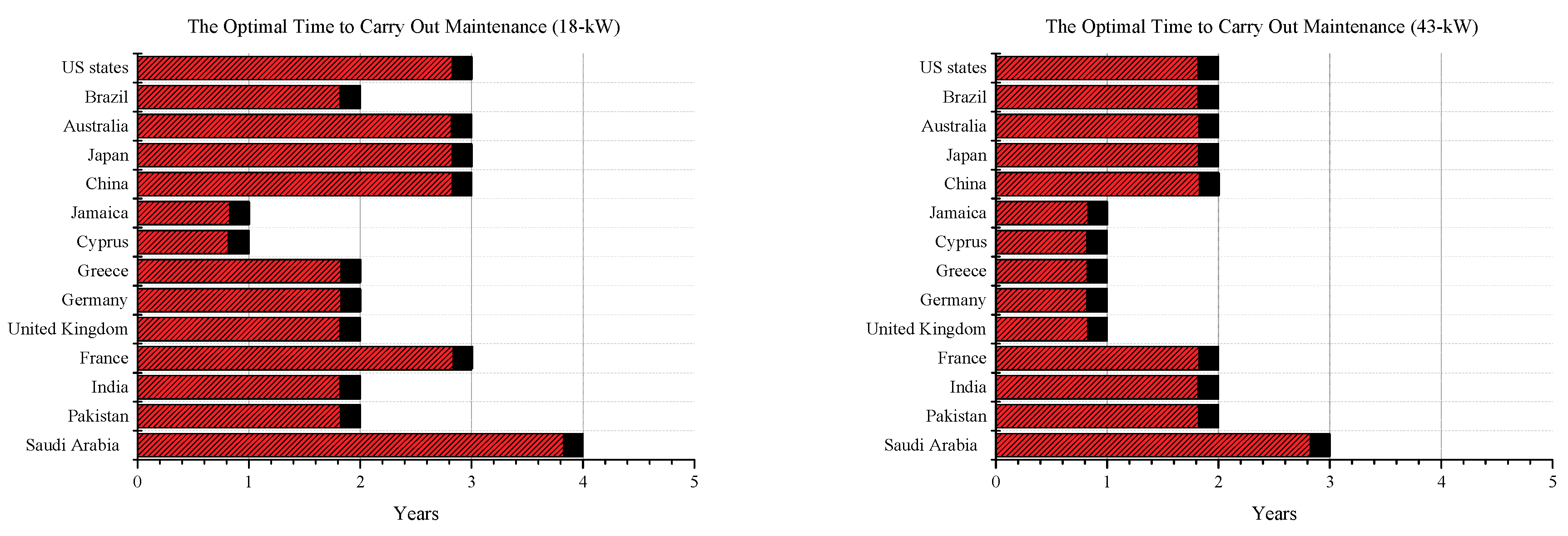
| Country | Cost of Swap/Replace Modules $/Time | Best Cost-Effective Maintenance Period Time | Additional Electric Revenue 18-kW ($) | Cost of Swap/Replace Modules $/Time | Best Cost-Effective Maintenance Period Time | Additional Electric Revenue 43-kW ($) |
|---|---|---|---|---|---|---|
| Saudi Arabia | 491.37 | 4 | 518.88 | 671.37 | 3 | 884.32 |
| Pakistan | 284.73 | 2 | 639.91 | 464.73 | 2 | 1433.74 |
| India | 277.49 | 2 | 552.97 | 457.49 | 2 | 1247.62 |
| France | 1023.41 | 3 | 1249.66 | 1203.41 | 2 | 1907.97 |
| United Kingdom | 781.8 | 2 | 1290.07 | 961.8 | 1 | 1165.19 |
| Germany | 1119.17 | 2 | 1457.83 | 1299.17 | 1 | 1346.38 |
| Greece | 500.82 | 2 | 1031.68 | 680.82 | 1 | 892.45 |
| Cyprus | 463.97 | 1 | 661.86 | 643.97 | 1 | 1667.59 |
| Jamaica | 279.06 | 1 | 658.42 | 459.06 | 1 | 1465.77 |
| China | 541.46 | 3 | 627.18 | 721.46 | 2 | 878.18 |
| Japan | 1069.4 | 3 | 2128.3 | 1249.4 | 2 | 3127.63 |
| Australia | 1290.53 | 3 | 1624.65 | 1470.53 | 2 | 2519.77 |
| Brazil | 430.58 | 2 | 656.73 | 610.58 | 2 | 1621.88 |
| US states | 727.31 | 3 | 890.81 | 907.31 | 2 | 1307.57 |
| Country | The Initial Value of Electric Revenue without Considering Labor Cost 18-kW ($) | Net Profit of Final Value Electric Revenue by Considering Labor Cost 18-kW ($) | The Initial Value of Electric Revenue without Considering Labor Cost 43-kW ($) | Net Profit of Final Value Electric Revenue by Considering Labor Cost 43-kW ($) |
|---|---|---|---|---|
| Saudi Arabia | 8897.92 | 9416.8 | 14,411.05 | 15,295.37 |
| Pakistan | 8143.86 | 8783.76 | 17,586.37 | 19,020.1 |
| India | 7314.39 | 7867.36 | 15,795.16 | 17,042.78 |
| France | 20,020.31 | 21,269.97 | 28,822.1 | 30,730.07 |
| United Kingdom | 18,248.27 | 19,538.34 | 19,703.24 | 20,868.43 |
| Germany | 22,697.23 | 24,155.06 | 24,506.93 | 25,853.31 |
| Greece | 13,497.69 | 14,529.37 | 14,573.89 | 15,466.33 |
| Cyprus | 9915.91 | 10,577.76 | 21,413.03 | 23,080.62 |
| Jamaica | 8256.97 | 8915.38 | 17,830.62 | 19,296.4 |
| China | 10,292.93 | 10,920.11 | 14,818.14 | 15,696.32 |
| Japan | 28,164.17 | 30,292.47 | 40,546.34 | 43,673.97 |
| Australia | 25,675.77 | 27,300.42 | 36,963.94 | 39,483.71 |
| Brazil | 9576.57 | 10,233.3 | 20,680.26 | 22,302.15 |
| US states | 14,251.75 | 15,142.56 | 20,517.43 | 21,825.01 |
| Case One (Swapping Age Modules) | Case Two (Swap/Replace Age Modules) | |||||||
|---|---|---|---|---|---|---|---|---|
| Country | Net Profit of Electric Revenue 18-kW ($) | Profits Return | Net Profit of Electric Revenue 43-kW ($) | Profits Return | Net Profit of Electric Revenue 18-kW ($) | Profits Return | Net Profit of Electric Revenue 43-kW ($) | Profits Return |
| Saudi Arabia | 18,484.95 | 2.39% | 33,953.36 | 0.97% | 9416.8 | 5.8% | 15,295.37 | 6.1% |
| Pakistan | 4229.61 | 2.72% | 8900.85 | 1.22% | 8783.76 | 7.9% | 19,020.1 | 8.1% |
| India | 3798.81 | 2.8% | 7997.1 | 1.26% | 7867.36 | 7.6% | 17,042.78 | 7.8% |
| France | 48,523.01 | 2.12% | 101,829.4 | 0.94% | 21,269.97 | 6.4% | 30,730.07 | 6.6% |
| United Kingdom | 37,909.82 | 2.32% | 79,630.39 | 1.04% | 19,538.34 | 7.01% | 20,868.43 | 5.9% |
| Germany | 58,940.38 | 2.25% | 123,766.96 | 1.01% | 24,155.06 | 6.4% | 25,853.31 | 5.5% |
| Greece | 21,030.55 | 2.52% | 44,216.77 | 1.13% | 14,529.37 | 7.6% | 15,466.33 | 6.1% |
| Cyprus | 20,599.76 | 2.69% | 43,344.03 | 1.21% | 10,577.76 | 7.7% | 23,080.62 | 7.8% |
| Jamaica | 8576.71 | 3.38% | 18,103.05 | 1.53% | 8915.38 | 7.9% | 19,296.4 | 8.2% |
| China | 17,819.18 | 2.03% | 44,919.83 | 1.05% | 10,920.11 | 6.1% | 15,696.32 | 5.9% |
| Japan | 48,757.98 | 2.02% | 122,907.76 | 1.04% | 30,292.47 | 7.6% | 43,673.97 | 7.7% |
| Australia | 62,230.07 | 2.04% | 149,353.52 | 1.01% | 27,300.42 | 6.3% | 39,483.71 | 6.8% |
| Brazil | 14,921.12 | 2.48% | 31,365.88 | 1.11% | 10,233.3 | 6.9% | 22,302.15 | 7.8% |
| US states | 29,607.26 | 2.08% | 72,562.45 | 1.05% | 151,42.56 | 6.2% | 21,825.01 | 6.3% |
Publisher’s Note: MDPI stays neutral with regard to jurisdictional claims in published maps and institutional affiliations. |
© 2020 by the authors. Licensee MDPI, Basel, Switzerland. This article is an open access article distributed under the terms and conditions of the Creative Commons Attribution (CC BY) license (http://creativecommons.org/licenses/by/4.0/).
Share and Cite
Alkahtani, M.; Hu, Y.; Alghaseb, M.A.; Elkhayat, K.; Kuka, C.S.; Abdelhafez, M.H.; Mesloub, A. Investigating Fourteen Countries to Maximum the Economy Benefit by Using Offline Reconfiguration for Medium Scale PV Array Arrangements. Energies 2021, 14, 59. https://doi.org/10.3390/en14010059
Alkahtani M, Hu Y, Alghaseb MA, Elkhayat K, Kuka CS, Abdelhafez MH, Mesloub A. Investigating Fourteen Countries to Maximum the Economy Benefit by Using Offline Reconfiguration for Medium Scale PV Array Arrangements. Energies. 2021; 14(1):59. https://doi.org/10.3390/en14010059
Chicago/Turabian StyleAlkahtani, Mohammed, Yihua Hu, Mohammed A Alghaseb, Khaled Elkhayat, Colin Sokol Kuka, Mohamed H Abdelhafez, and Abdelhakim Mesloub. 2021. "Investigating Fourteen Countries to Maximum the Economy Benefit by Using Offline Reconfiguration for Medium Scale PV Array Arrangements" Energies 14, no. 1: 59. https://doi.org/10.3390/en14010059
APA StyleAlkahtani, M., Hu, Y., Alghaseb, M. A., Elkhayat, K., Kuka, C. S., Abdelhafez, M. H., & Mesloub, A. (2021). Investigating Fourteen Countries to Maximum the Economy Benefit by Using Offline Reconfiguration for Medium Scale PV Array Arrangements. Energies, 14(1), 59. https://doi.org/10.3390/en14010059