Dynamic Modeling of an Offshore Floating Wind Turbine for Application in the Mediterranean Sea

Abstract

Wind power is emerging as one of the most sustainable and low-cost options for energy production. Far-offshore floating wind turbines are attractive in view of exploiting high wind availability sites while minimizing environmental and landscape impact. In the last few years, some offshore floating wind farms were deployed in Northern Europe for technology validation, with very promising results. At present time, however, no offshore wind farm installations have been developed in the Mediterranean Sea. The aim of this work is to comprehensively model an offshore floating wind turbine and examine the behavior resulting from a wide spectrum of sea and wind states typical of the Mediterranean Sea. The flexible and accessible in-house model developed for this purpose is compared with the reference model FAST v8.16 for verifying its reliability. Then, a simulation campaign is carried out to estimate the wind turbine LCOE (Levelized Cost of Energy). Based on this, the best substructure is chosen and the convenience of the investment is evaluated.

1. Introduction

The improvement of technology and the use of larger turbines have led offshore wind projects to reach capacity factor (CF) levels between 40% and 50%. CF describes the average power output over the year relative to the maximum rated power capacity. These values enable wind energy to have very competitive Levelized Cost of Energy (LCOE), often already comparable to that of fossil fuel power plants. In addition, wind turbines typical production profiles are partially complementary to those of photovoltaic (PV) systems, with beneficial effects in the reduction of the overall energy supply cost. Offshore wind power today has a global capacity of 23 GW (80% of which in Europe), but still constitutes only the 0.3% of global electricity production. Despite this, it has the potential to become one of the best green alternatives in the global energy supply [1,2]. To fully understand the importance of this energy resource, it is useful to observe that the best offshore wind sites could provide more than the total amount of electricity consumed worldwide today. Considering that the current annual global demand amounts to 23,000 TWh [1], it is necessary to analyze the available technical potential by distinguishing the wind turbine offshore structures into two groups: bottom-fixed structures and floating platforms. The former are cheaper installations, located at a sea depth lower than 50–60 m, over to which the installation costs would make the investment inconvenient [1,2,3,4]. The global technical potential of the areas suitable for this type of structures is approximately 87,000 TWh per year [1,3]. The latter, on the other hand, can also be installed in areas very far from the coast, with sea depth higher than 60 m. This makes the costs of these structures much higher than the fixed ones, but they allow to reach areas with a global technical potential of 330,000 TWh. Many industries are pushing towards the latter solution. In this way, through technological development, costs would decrease thus making this potential accessible.

To date, the leader in offshore wind is Europe, specifically Northern Europe [5,6,7] which generally has huge wind resource availability. The largest wind farms installed in these areas are Hornsea (situated in UK with a capacity of 1218 MW) [8], Gemini Wind Farm (situated in Netherlands with a capacity of 600 MW) [9], Gode Wind (situated in Germany with a capacity of 600 MW) [10]. As for the Mediterranean, instead, there are no operating offshore wind farms, especially because of its steep bathymetric profile and generally deep waters; for this reason it is important to start planning an offshore wind farm project in the Mediterranean, in order to meet the growing electricity needs of the area with cost-efficient and low environmental impact renewable technologies. Since the Mediterranean Sea has different characteristics from the North Sea, it is important to explore different substructure concepts [11,12] with respect to those that were already deployed, in order to identify those that best fit the characteristic sea conditions. Once a small group of substructure concepts has been identified, a dynamic model is needed to simulate the behavior of each concept, so as to select the best in terms of performance and reliability.

The approaches to the modeling of floating offshore wind turbines can be categorised according to the required accuracy of the model to be developed, taking into consideration the role that the model will have in the design phase. Very simple models, which therefore require a minimum computational load, are generally used in the evaluation of the capacity factor of a given installation site [13]. They are generally represented by a simple power curve, through which it is possible to derive the estimated annual power, starting from the wind distribution in a given site. Models of much higher accuracy are those that take into account the interaction between hydrodynamic and aerodynamic effects, such as FAST [14,15], OrcaFlex [16] and the model that is presented as follows; also, it is worth mentioning the QBlade software [17,18,19], that is exclusively related to wind turbines aerodynamic but has similar characteristics. All these models return quite precise results, at the expenses of a medium-to-high computational burden. In particular, the FAST model was used for comparison thanks to its proven and well-established reliability. Finally, CFD (Computational Fluid Dynamics) high-fidelity models such as OpenFoam [20], that are based on the resolution of Navier-Stokes equations, guarantee very high accuracy, but are characterised by huge computational burden. For these characteristics, they are mostly used in the verification phase of new structures.

FAST is a computational-efficient simulator and is the reference software for the simulation of offshore floating wind turbines [21,22,23]. Nevertheless, it is characterised by a low accessibility because of its complex background code. In the work hereby presented, we developed and applied a new comprehensive modeling tool for the planning and design phase of offshore floating wind turbine projects. In order to enable high adaptability and flexibility of use of the tool, we developed the in-house model on the programming language Simulink-MATLAB [24], which, thanks to its intuitive structure and user friendliness, makes the tool easily programmable and editable.

The following steps were followed for the full definition of the model:

• Construction of a state of the art mathematical model for onshore wind turbines, in order to implement the aerodynamics and finally verify the results with FAST, in terms of control on the blade pitch, generated power and loads discharged at the tower base.
• Construction of a state of the art mathematical model for a platform immersed in water, in order to implement hydrodynamics and finally verify the results with FAST, in terms of hydrostatic and hydrodynamic loads, moorings and displacements of the hull.
• Combination of the aerodynamics and hydrodynamics macro-blocks: the loads at the base of the tower act on the hull, the movements of the platform influence the orientation of the turbine which is integral with it.

Once the in-house model was verified by comparing it with FAST v8.16, it was applied through a genetic algorithm to the optimization of the geometrical dimensions of two floaters concepts, with the aim of minimizing the investment cost [25]. Then, the CF and LCOE of a 5 × 5 MW wind farm were calculated for the two concepts, leading to the identification of the best platform. Finally, the convenience of the investment compared to an onshore case study was discussed, with a view on future developments of the offshore wind sector.

The paper is structured as follows. Materials and methods (Section 2) describes the considered offshore floating wind turbine and floating platforms: Section 2.1 shows the overall modeling framework; Section 2.2 deals with the hydrodynamic modeling of the floating platform; Section 2.3 analyses the mooring loads acting on the floating platform and Section 2.4 explains the aerodynamic modeling of the wind turbine. In Results (Section 3), Section 3.1 provides bases for the installation site identification; Section 3.2 validates the developed model; Section 3.3 describes the choice of the most suitable floating platform. Finally, Section 4 contains conclusions.

2. Materials and Methods

The overall system under study consists of four main elements: NREL 5-MW wind turbine, floater (optimized hexafloat or optimized spar), mooring lines, surrounding environment.

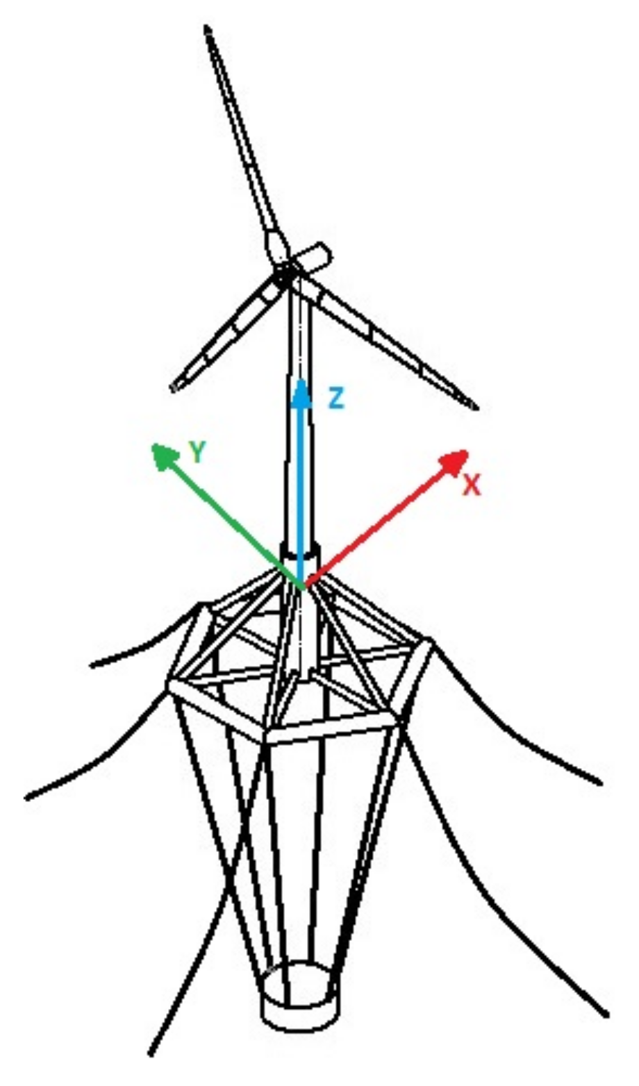
The Fixed Reference Axis (FRA) frame $Oxyz$, represented in Figure 1, is defined as a right-handed reference frame with the origin O identified as the intersection between the system vertical y axis of “symmetry” at rest and the mean water plane, the z axis pointing upwards and the x axis pointing backwards downwind; this frame is fixed in the space and thus represents an inertial reference. The Local Structure Axis (LSA) frame $Gxyz$ has its origin coincident with the FRA; it is employed to describe the motions of the system in the FRA.

Table 1. Undistributed blade aerodynamic and structural properties.

Mass	4605 t
Displacement	5250 m${}^3$
Draft	12 m
Center of gravity from the FRA	(0, 0, −55) m
Roll moment of inertia	34,803,381,981 kg m${}^2$
Pitch moment of inertia	1,579,004,565 kg m${}^2$
Yaw moment of inertia	34,818,228,666 kg m${}^2$

summarizes the properties of the complete system.

2.1. Dynamic Modeling

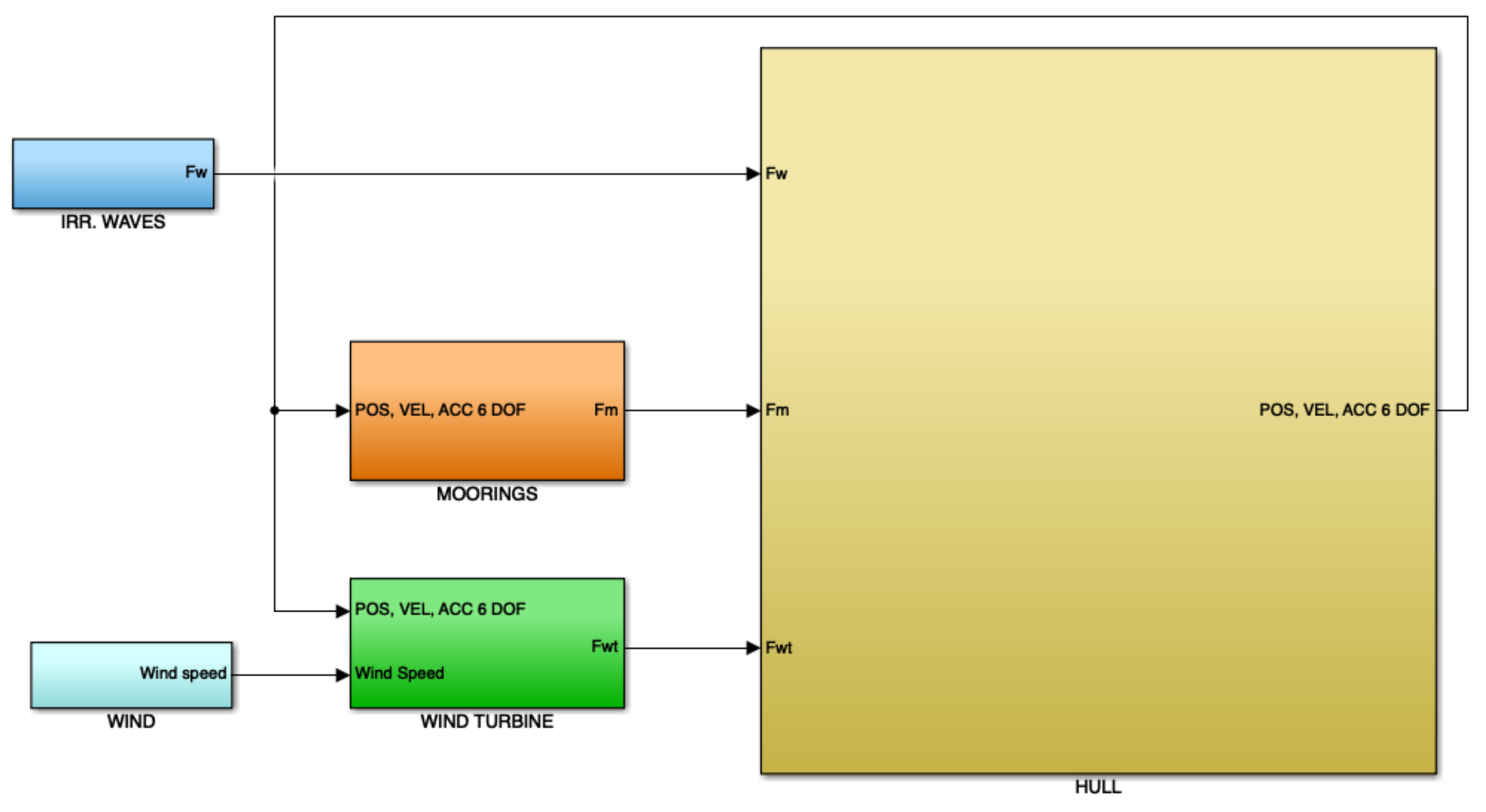
Figure 2 represents the overall implementation in MATLAB-Simulink [26] of the complete system.

This is divided into two macroblocks: hydrodynamics (which represents the hull immersed in water and held in place by the moorings) and aerodynamics (which represents the turbine). The connection between the two macroblocks is represented by the loads at the base of the turbine, which act on the hull and influence its movements.

As shown in Figure 2, the system is composed by several blocks representing the different components:

• Waves: for each timestep it provides the loads in the 6-DOFs acting on the hull and derived from waves.
• Wind: for each timestep it provides the wind speed components on the three axis of the FRA (U-wind, V-wind, W-wind).
• Wind turbine: for each timestep it provides loads in the 6-DOFs acting at the turbine tower base on the hull. It takes as input wind speeds and 6-DOFs positions of the hull, from which it calculates loads on the turbine that generate power and reaction loads at the base.
• Moorings: for each timestep it provides loads in the 6-DOFs acting on the hull due to mooring lines for stability maintenance. Moorings block outputs depend on hull 6-DOFs position.
• Hull: for each timestep it takes loads by waves, moorings and wind turbine. Through hydrodynamics laws 6-DOFs position are detected.

Note that mooring and wind turbine loads, acting on hull, depend on hull position in the previous timestep (that is the output of hull block): there is a feedback of 6-DOFs position.

2.2. Hydrodynamics

Waves loads (${\mathit{F}}_{\mathit{FK}}+{\mathit{F}}_{\mathit{D}}$), moorings loads (${\mathit{F}}_{\mathit{moor}}$) and tower base loads (${\mathit{F}}_{\mathit{wt}}$) act on the hull. The hull movement in water then gives rise to other effects such as drag (${\mathit{F}}_{\mathit{drag}}$), radiation (${\mathit{F}}_{\mathit{R}}$) and hydrostatic loads (${\mathit{F}}_{\mathit{hst}}$) [27].

Newton’s law of motion for a floating body is:

$$\mathbf{M}\ddot{\mathit{x}}={\mathit{F}}_{\mathit{hst}}+{\mathit{F}}_{\mathit{FK}}+{\mathit{F}}_{\mathit{D}}+{\mathit{F}}_{\mathit{R}}+{\mathit{F}}_{\mathit{drag}}+{\mathbf{F}}_{\mathbf{moor}}+{\mathit{F}}_{\mathit{wt}}$$

(1)

The regular incoming wave, considered on the vertical axis of the structure, has the form:

$$\eta \left(t\right)=a{e}^{-j\omega t}$$

then the excitation load have analogue structure. Moreover, since the Froude-Krylov and diffraction loads are those associated with the incident wave, they determine the excitation load:

$${\mathit{F}}_{\mathit{exc}}\left(t\right)={\mathit{F}}_{\mathit{FK}}+{\mathit{F}}_{\mathit{D}}=a\left|\mathit{f}\left(\omega \right)\right|e^{-j(\omega t+\angle \mathit{f}(\omega \left)\right)}$$

(2)

where the complex excitation load $\mathit{f}$ carries the Froude-Krylov coefficients, excitation load amplitude and phase with respect to that of the incident wave, as real and complex part, respectively. So, the excitation load can be written in the frequency domain as:

$${\mathit{F}}_{\mathit{exc}}\left(\omega \right)=a\mathit{f}\left(\omega \right)$$

(3)

By considering small-amplitude motions around a mean equilibrium floating position and neglecting non-linear terms, the equation of motion in the frequency domain becomes:

$$\left[-{\omega }^2\left(\mathbf{M}+\mathbf{A}\left(\omega \right)\right)+j\omega \mathbf{B}\left(\omega \right)+\mathbf{K}\right]\mathit{x}\left(\omega \right)={\mathit{F}}_{\mathbf{exc}}\left(\omega \right)$$

(4)

The added-mass $\mathbf{A}\left(\omega \right)$, radiation-damping $\mathbf{B}\left(\omega \right)$ and hydrostatic-stiffness $\mathbf{K}$ matrices, along with the Froude-Krylov coefficient vector $\mathit{f}\left(\omega \right)$, are extrapolated by the analysis performed by ANSYS Aqwa [28] in the frequency domain, for a given direction of the incident wave.

Finally, the mass & inertia matrix on reference frame (0,0,0) is defined as follows:

$$\mathbf{M}=\left[\begin{array}{cccccc}m& 0& 0& 0& m{z}_g& -m{y}_g\\ 0& m& 0& -m{z}_g& 0& m{x}_g\\ 0& 0& m& m{y}_g& -m{x}_g& 0\\ 0& -m{z}_g& m{y}_g& I_{xx}& I_{xy}& I_{xz}\\ m{z}_g& 0& -m{x}_g& I_{yx}& I_{yy}& I_{yz}\\ -m{y}_g& m{x}_g& 0& I_{zx}& I_{zy}& I_{zz}\end{array}\right]$$

where m is the full-system mass, I are moments of inertia, $(x_g,y_g,z_g)$ is the distance of the center of mass from the reference frame.

The representation of the equation of motion in the time domain is due to Cummins [29]:

$$(\mathbf{M}+{\mathbf{A}}_{\infty })\ddot{\mathit{x}}\left(t\right)+{\int }_0^t\mathbf{K}{}_{\mathit{R}}(t-\tau )\dot{\mathit{x}}\left(\tau \right)d\tau +\mathbf{K}\mathit{x}\left(t\right)-{\mathit{F}}_{\mathit{drag}}\left(t\right)={\mathit{F}}_{\mathit{exc}}\left(t\right)+{\mathit{F}}_{\mathit{moor}}\left(t\right)+{\mathit{F}}_{\mathit{wt}}\left(t\right)$$

(5)

Ogilvie (1964) [30] established the relationship between the frequency- and the time-domain representations, Equations (4) and (5), by using the Fourier transform:

$$\begin{array}{cc}\hfill & \mathbf{A}\left(\omega \right)={\mathbf{A}}_{\infty }-\frac{1}{\omega }{\int }_0^{\infty }\mathbf{K}{}_{\mathit{R}}\left(t\right)sin\left(\omega t\right)dt\hfill \end{array}$$

(6)

$$\begin{array}{cc}\hfill & \mathbf{B}\left(\omega \right)={\int }_0^{\infty }\mathbf{K}{}_{\mathit{R}}\left(t\right)cos\left(\omega t\right)dt\hfill \end{array}$$

(7)

The infinite limit of Equation (6) expresses the meaning of the infinite-frequency added mass ${\mathbf{A}}_{\infty }$:

$${\mathbf{A}}_{\infty }=\underset{\omega \to \infty }{lim}\mathbf{A}\left(\omega \right)$$

Fourier transforms also provide the time- and frequency-domain representation of the retardation function $\mathbf{K}{}_{\mathit{R}}$:

$$\begin{array}{cc}\hfill & \mathbf{K}{}_{\mathit{R}}\left(t\right)=\frac{2}{\pi }{\int }_0^{\infty }\mathbf{B}\left(\omega \right)cos\left(\omega t\right)d\omega \hfill \end{array}$$

(8)

$$\begin{array}{cc}\hfill & \mathbf{K}{}_{\mathit{R}}\left(j\omega \right)={\int }_0^{\infty }\mathbf{K}{}_{\mathbf{R}}\left(t\right)e^{-j\omega t}d\omega =\mathbf{B}\left(\omega \right)+j\omega \left[\mathbf{A}\left(\omega \right)-{\mathbf{A}}_{\infty }\right]\hfill \end{array}$$

(9)

The obsequious implementation of the time-domain representation Equation (5) for simulations proves to be highly time- and memory-demanding because of the presence of the convolution integral associated with the radiation damping, hence approximations have been developed. In this work is used FOAMM, which is an algorithm based on finite order moment matching [31]. It proposes the approximation through linear-time-invariant state-space model (LTI SSM), a set of linear ordinary differential equations:

$$\mathit{\mu }\left(t\right)\doteq {\int }_0^t\mathbf{K}{}_{\mathit{R}}(t-\tau )\dot{\mathit{x}}\left(\tau \right)d\tau \approx \left\{\begin{array}{c}\dot{\mathit{u}}\left(t\right)={\mathbf{A}}_{\mathbf{ss}}\mathit{u}\left(t\right)+{\mathbf{B}}_{\mathbf{ss}}\dot{\mathit{x}}\left(t\right)\hfill \\ \mathit{\mu }\left(t\right)={\mathbf{C}}_{\mathbf{ss}}\mathit{u}\left(t\right)\hfill \end{array}\right.$$

(10)

where $\mathit{x}\left(t\right)$ represents the input vector, $\mathit{\mu }\left(t\right)$ the output vector and $\mathit{u}\left(t\right)$ the state vector of the state-space model, whose parameters matrices ${\mathbf{A}}_{\mathbf{ss}}$, ${\mathbf{B}}_{\mathbf{ss}}$ and ${\mathbf{C}}_{\mathbf{ss}}$ are to be estimated through model identification.

2.2.1. Irregular Waves

Real waves are the result of systems of winds blowing on the water surface. Swells are usually long-crested nearly-unidirectional sinusoidal waves because they were generated by the wind in a previous space or time, but local winds still affect the sea surface, producing short-crested multidirectional highly-irregular waves (sea). For this reason, the sea surface may be expressed as a Fourier series, a superposition of-theoretically infinite-regular waves components with different height, frequency, wavelength and random phase (Figure 3). For a single direction, this takes the form:

$$\eta (x,t)=\sum _N^{n=1}{a}_{n}sin({\omega }_{n}t-k_{n}x+{\phi }_n)$$

(11)

where the subscripts n indicate that the wave parameters are relative to the n-th component of the summation along N.

This summation is finite because the contribution of the the n-th wave becomes less significant for increasing frequencies. A wave spectral density function $S_{\eta }\left({\omega }_n\right)$, calculated as the variance function of the waves amplitudes $a_n$, carries information about the significance of each wave component-identified by the n-th frequency ${\omega }_n$-in the signal; narrower curves represent waves closer to be regular.

Standard Wave Spectra

The JONSWAP (Joint North Sea Wave Project) spectrum [33], developed for the North Sea coastal wind-generated waves, is based on the significant wave height $H_s$ and a reference wave period $\overline{T}$ ($T_1$, $T_2$ or $T_p$):

$$S_{\eta }\left(\omega \right)=\frac{320H_s^2}{T_p^4}{\omega }^{-5}{\gamma }^A{e}^{-{\displaystyle \frac{1950}{T_p^4}}{\omega }^{-4}}$$

(12)

with:

$$\begin{array}{cc}\hfill \gamma & =3.3\mathrm{peak}\mathrm{enhancement}\mathrm{factor}\hfill \end{array}$$

(13)

$$\begin{array}{cc}\hfill A& =exp\left(-{\left(\frac{\frac{\omega }{{\omega }_p}-1}{\sigma \sqrt{2}}\right)}^2\right)\hfill \end{array}$$

(14)

$$\begin{array}{cc}\hfill {\omega }_p& =\frac{2\pi }{T_p}\mathrm{peak}\mathrm{frequency}\hfill \end{array}$$

(15)

$$\begin{array}{cc}\hfill \sigma & =\left\{\begin{array}{cc}0.07\hfill & \omega <{\omega }_p\hfill \\ 0.09\hfill & \omega <{\omega }_p\hfill \end{array}\right.\hfill \end{array}$$

(16)

The transformation to time series requires the statistical description of the wave as spectrum to be transformed into a deterministic time history of wave elevation, without losing the statistical properties of the original spectrum, that is the energy density. This is done by filling in all the constants of the already-presented Equation (11), that are the amplitude $a_n$, the wave number $k_n$, and the phase ${\phi }_n$, for each frequency component ${\omega }_n$, usually chosen at evenly-spaced intervals $\Delta {\omega }_n$ along the frequency axis. The wave amplitudes $a_n$ are determined from the notion that the finite area under the relative $\Delta {\omega }_n$ interval of the spectrum, $S_{\eta }\left(\omega \right)\Delta \omega$, represents the variance of the n-th wave component:

$$a_n=\sqrt{2}\sqrt{S_{\eta }\left(\omega \right)\Delta \omega }$$

(17)

The wave numbers $k_n$ are obtained from the given frequency ${\omega }_n$ using the dispersion relation. Since the phase angles ${\phi }_n$ were discarded when the wave spectrum $S_{\eta }\left(\omega \right)$ was generated from the irregular wave history, these are now randomly selected in the linear space in the range $0\le {\phi }_n\le 2\pi$. The exact value of phase angle correlated to the given frequency does not influence the statistics of the newly-generated time history, therefore the new random set of ${\phi }_n$ values produce an instantaneously-different but statistically- (and thus energetically-) equivalent time record.

2.2.2. Hydrostatic ‘Restoring’ Load

As stated by Archimede’s principle, any body, fully or partially submerged in still water, receives an upward buoyant load equal to the weight of the fluid displaced by the body and applied on the center of buoyancy ${\overrightarrow{X}}_B$ (defined with respect of the center of gravity reference):

$${\overrightarrow{F}}_{buoy}=-\rho V_0\overrightarrow{g}$$

where $\rho$ is the water density, $V_0$ is the submerged volume, $\overrightarrow{g}$ the gravitational acceleration. The buoyancy force is the vertical component of the hydrostatic force. The hydrostatic force and moment are the actions resulting from the hydrostatic pressure field applied on the wetted surface:

$$\begin{array}{cc}\hfill {\overrightarrow{F}}_{hs}& =-\underset{S_0}{\int }{p}_{hs}\overrightarrow{n}dS\hfill \\ \hfill {\overrightarrow{M}}_{hs}& =-\underset{S_0}{\int }{p}_{hs}(\overrightarrow{r}\times \overrightarrow{n})dS\hfill \end{array}$$

where $p_{hs}\left(z\right)=-\rho gz$ is the hydrostatic pressure, $\overrightarrow{r}$ the position vector of a surface point with respect to the center of gravity (COG), $\overrightarrow{n}$ the unit vector of the buoyant surface pointing outwards, $S_0$ the wetted surface. When the body is in its hydrostatic equilibrium position, the hydrostatic force balances the gravity force and the hydrostatic moment balances the moment of the distributed gravity force about the center of gravity, which translates into the center of gravity and the center of buoyancy being vertically aligned.

Horizontal translations or rotation on a horizontal plane take the floating body to a new equilibrium condition, therefore surge, sway and yaw motions ($x,y$ and $rz$) induce neutral equilibrium. Heave motion (z) does not perturb the equilibrium condition, which is stable. Roll and pitch motions ($rx$ and $ry$), conversely, induce moments about the center of gravity, so the equilibrium may be stable, neutral or unstable.

Considering the overall motions around a mean equilibrium floating position, the buoyancy load is balanced by the weight, and the remaining actions result from the displacements z, $rx$, $ry$: the change in load due to the change in the submerged volume of the vessel as it heaves, rolls and pitches (waterplane area effects), and the change in moment caused by movement of the vessel’s centre of gravity and centre of buoyancy as it rolls and pitches (moment arm effects). Adopting the small amplitude approximation, the submerged volume and the wetted surface are constant and equal to the ones at rest, therefore the coefficients relating forces and moments to displacements are constant as well. In this way, waterplane area effects can be neglected, while moment arm effects can be described by a linear relation. Under this assumptions, the hydrostatic restoring loads is composed of hydrostatic loads ${\mathit{F}}_{\mathit{hsr}}$, restoring moments ${\mathit{F}}_{\mathit{restoring}}$ and non-linear loads ${\mathit{F}}_{\mathit{non}-\mathit{linear}}$:

$${\mathit{F}}_{\mathit{hsr}}=-\mathbf{K}\mathit{x}+{\mathit{F}}_{\mathit{restoring}}+{\mathit{F}}_{\mathit{non}-\mathit{linear}}$$

(18)

Being $\mathit{x}$ the vector containing the displacements of the floater COG relatively to the FRA and $\mathbf{K}$ the hydrostatic stiffness matrix:

$$\mathbf{K}=\left[\begin{array}{cccccc}0& 0& 0& 0& 0& 0\\ 0& 0& 0& 0& 0& 0\\ 0& 0& K_{33}& K_{34}& K_{35}& 0\\ 0& 0& K_{43}& K_{44}& K_{45}& K_{46}\\ 0& 0& K_{53}& K_{54}& K_{55}& K_{56}\\ 0& 0& 0& 0& 0& 0\end{array}\right]$$

where $K_{34}=K_{43}$, $K_{45}=K_{54}$ and $K_{35}=K_{53}$. Positive coefficients are associated with stable equilibrium (restoring forces and moments), null coefficients are associated with neutral equilibrium and negative coefficients are associated with unstable equilibrium (capsizing moments) [34].

The hydrostatic stiffness matrix is simplified by the following considerations:

• the $xz$ and the $yz$ planes are symmetry planes, so $K_{34}=K_{35}=K_{45}=0$. This approximation holds because the elements violating symmetry-the rotating blades and the nacelle-have negligible masses and their centres of mass are very close to the z axis
• in the small amplitude approximation, the centre of buoyancy and the centre of gravity stay vertically aligned, so $K_{46}=K_{56}=0$.

The resulting matrix is diagonal and has only three non-zero terms ($K_{33}$, $K_{44}$, $K_{55}$):

$$\mathbf{K}=\left[\begin{array}{cccccc}0& 0& 0& 0& 0& 0\\ 0& 0& 0& 0& 0& 0\\ 0& 0& K_{33}& 0& 0& 0\\ 0& 0& 0& K_{44}& 0& 0\\ 0& 0& 0& 0& K_{55}& 0\\ 0& 0& 0& 0& 0& 0\end{array}\right]$$

The other contribution to hydrostatic loads is given by the gravity restoring moments $M_x$ and $M_y$ related to gravity that leads to straightening the inclined system by exploiting the weight force (located in the center of mass, under the Still Water Level (SWL)). Considering the total mass m and the istantaneous position [35] of the center of mass ($x_g,y_g,z_g$):

$$M{x}_{restoring}=-mg{y}_g$$

(19)

$$M{y}_{restoring}=mg{x}_g$$

(20)

Finally, non-linear loads take into account the inertial loads due to the fact that the LSA is not in the center of mass. Its formulation for the 3 forces ${\mathit{F}}_{\mathit{non}-\mathit{linear}}$ and the 3 moments ${\mathit{M}}_{\mathit{non}-\mathit{linear}}$ is given by:

$${\mathit{F}}_{\mathit{non}-\mathit{linear}}=\mathsf{\Omega }\times (\mathsf{\Omega }\times r_{cm}m)$$

(21)

$${\mathit{M}}_{\mathit{non}-\mathit{linear}}=\mathsf{\Omega }\times \mathit{I}\mathsf{\Omega }$$

(22)

where $\mathsf{\Omega }=(rx,ry,rz)$: platform rotations, m: total mass, $r_{cm}=(x_g,y_g,z_g)$: center of mass in LSA and $\mathit{I}$: inertia matrix.

2.2.3. Froude-Krylov Load

The Froude-Krylov load is the resultant load of the unsteady pressure field generated by the undisturbed incident wave pressure field:

$${\mathit{F}}_{\mathit{FK}}=-\underset{S_0\left(t\right)}{\int }{p}_I\overrightarrow{n}dS$$

(23)

where $\overrightarrow{n}$ is the surface normal unit vector, $S_0\left(t\right)$ the instantaneous wetted surface and $p_I$ the incoming wave pressure field. Linear codes differ from non-linear ones for the assumption of constant wetted surface, which is legitimate for small body motions.

2.2.4. Diffraction Load

The diffraction load is caused by the disturbance wave due to the interaction between the incident wave and the body, considering $p_D$ the unsteady pressure field associated with the diffracted wave field. It may also be expressed through the diffraction loads impulse response function (${\mathit{K}}_{\mathit{D}}$):

$${\mathit{F}}_{\mathit{D}}=-\underset{S_0\left(t\right)}{\int }{p}_D\mathit{n}dS=-{\int }_0^t{\mathit{K}}_{\mathbf{D}}(t-\tau )\eta \left(\tau \right)d\tau$$

The diffraction loads ${\mathit{F}}_{\mathit{D}}$, combined with Froude-Krylov loads ${\mathit{F}}_{\mathit{FK}}$, constitute the wave loads ${\mathit{F}}_{\mathit{exc}}$ (Equation (2)).

2.2.5. Radiation Load

The unsteady motion of the platform originates radiated waves whose associated unsteady pressure field $p_R$ gives the radiation load as the resultant action on the body:

$${\mathit{F}}_{\mathit{R}}=-\underset{S_0\left(t\right)}{\int }{p}_R\mathit{n}dS$$

The radiation problem was analysed by Cummins [29], who gives the following expression:

$${\mathit{F}}_{\mathit{R}}\left(t\right)=-\mathbf{A}{}_{\infty }\ddot{\mathit{x}}-{\int }_0^t\mathbf{K}{}_{\mathit{R}}(t-\tau )\dot{\mathit{x}}\left(\tau \right)d\tau$$

(24)

The first term in Equation (24) is a frequency-independent inertial term which accounts for the water mass carried by the body in its motion, thus $\mathbf{A}{}_{\infty }$ is a constant positive definite matrix named added mass matrix. The second term is a convolution integral over velocity $\dot{\mathit{x}}\left(t\right)$, representing a source of damping; the impulse response function matrix $\mathbf{K}{}_{\mathit{R}}$ is called memory function matrix. The convolution integral is replaced by the state-space model (Equation (10)).

2.2.6. Drag Load

Drag load takes into account the effects of damping due to fluid viscosity and to flows detaching from the buoyant and dissipating energy into vortices. Although linear models do not consider these phenomena because of their base hypotheses, extra damping is required in order to accurately model the damping in a real system. These non-linearities may be integrated by a model of quadratic drag force distributed along the platform profile. By identifying nodes along z, it is possible to define the entity of the distributed load at that particular point, and then integrate along the entire z profile of the platform to derive forces and moments in the FRA. The discretization of the nodes has a variable step, gradually becoming finer towards the water level, where the speeds $V_x$ and $V_y$ are greater, and therefore the drag actions are more important.

The force per unit of length (N/m) at a particular node is defined as:

$$\begin{array}{c}\hfill \frac{d{F}_x}{dz}=\frac{1}{2}{C}_d\rho D{V}_x\sqrt{V_x^2+V_y^2}\\ \hfill \frac{d{F}_y}{dz}=\frac{1}{2}{C}_d\rho D{V}_y\sqrt{V_x^2+V_y^2}\end{array}$$

where $C_d$ is the drag coefficient, taken 0.6 which is the typical coefficient for a cylinder [36], $\rho =1025$ kg/m${}^3$ is the density of water, D is the platform diameter, $V_x$ and $V_y$ are the relative velocities between fluid particles and structure. In fact, these velocities are depth-dependent and include contributions both from wave/current kinematics and structural motions.

To calculate the total integrated force and moment in FRA (relative to the waterline), these must be integrated along the platform profile (from the lower end of the platform $z=-L$ to the water plan $z=0$):

$$\left\{\begin{array}{c}{F}_x={\int }_{-L}^0\frac{d{F}_x}{dz}dz\hfill \\ F_y={\int }_{-L}^0\frac{d{F}_y}{dz}dz\hfill \\ M_x={\int }_{-L}^0-z\frac{d{F}_y}{dz}dz\hfill \\ M_y={\int }_{-L}^{0}z\frac{d{F}_x}{dz}dz\hfill \end{array}\right.$$

(25)

2.3. Moorings

In offshore wind turbines, the mooring system is designed in order to prevent the system from drifting under the action of waves, currents and wind and to increase rotational stability. In fact, in order to have the turbine orientation stably in the direction of maximum exploitation of the wind resource, rotational stability is required. The solution hereby implemented is a catenary mooring system consisting of a set of six lines evolving radially and uniformly distributed in the 360${}^{\circ }$ of the water plane, to keep the floater in position. However, it is important to remark that, because of the difficult representation of the bind responses related to moorings, experimental testing in this field is a key element of floating platforms development [37].

The sea depth of the case study is about 120 m. The single lines are metal chain, this is the simplest and cheaper solution and gives a good stiffness. The mooring system properties are summarized in

Table 2. Mooring lines properties.

number of mooring lines	6
angle between adjacent lines	60${}^{\circ }$
seabed depth	120 m
mooring leg composition	chain
unstretched lengths	473.3 m
type	chainup
diameter	80.9 mm
mass per unit length	138.7 kg/m
min. breaking load	3380 kN
axial stiffness	1071 MN
cable/seabed friction coefficient	1

.

The modeling of the mooring lines is made basing on MAP++ theory, a multisegmented quasi-static (MSQS) mooring model available in FAST v8.16 that was developed by Marco Masciola with both the National Renewable Energy Laboratory (NREL) and the American Bureau of Shipping (Masciola, Jonkman, and Robertson 2013). “It is a relatively simple model that allows for a robust, first-pass evaluation of a mooring system by considering the average mooring line loads and nonlinear geometric restoring for both catenary and taut mooring systems” [38].

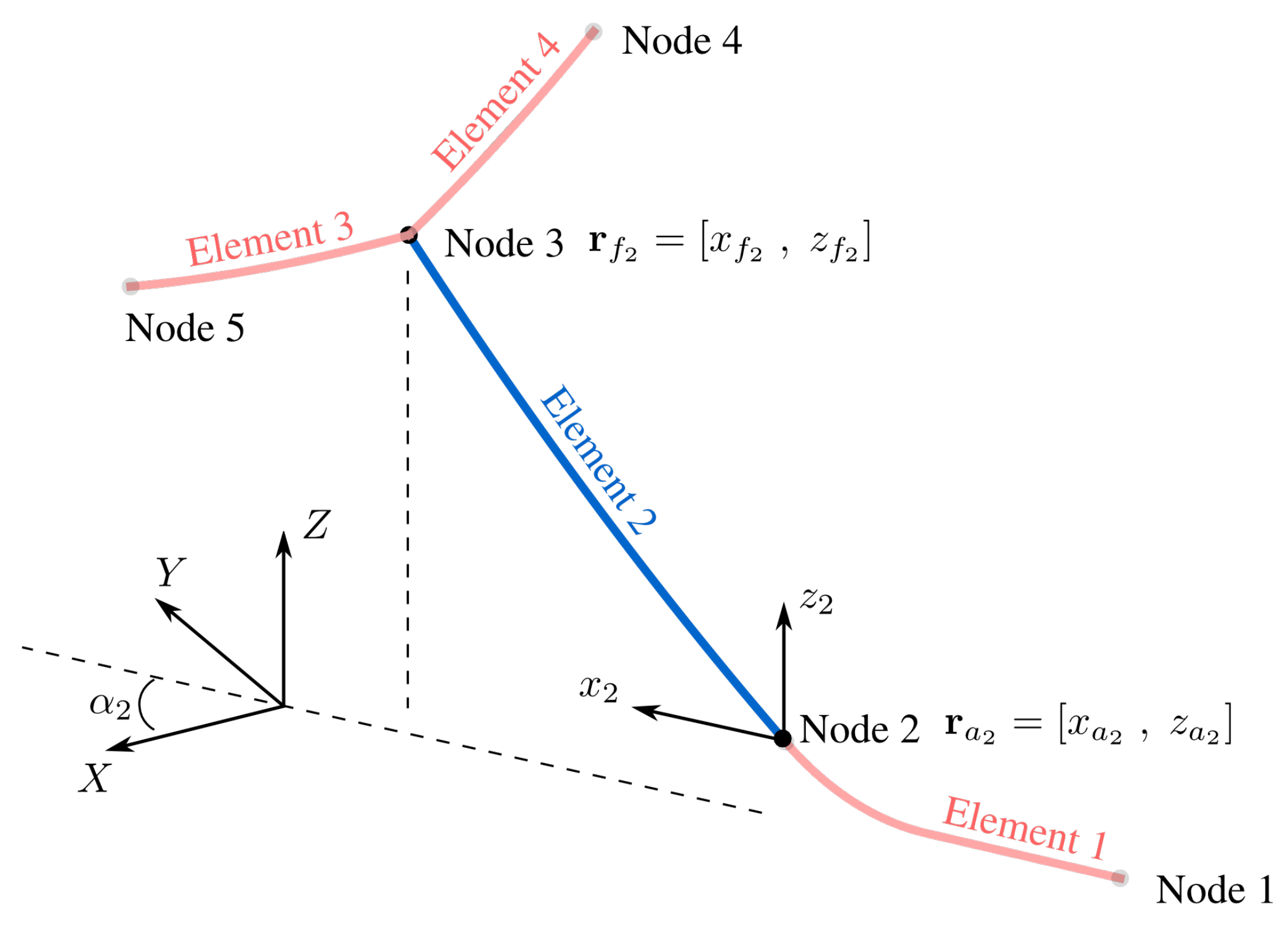
Assuming a quasi-static approach, the motion of the system during a given time step is considered uniform and linear between two static positions; for every timestep, the loads on the systems are assumed constant [39]. This method ignores the dynamic effects on the mooring, omitting the motion dependency of mass, damping and fluid acceleration on the system [40]. This assumption is justified by the fact that the platform has limited movement. Moreover, MAP++ does not consider bending and torsional cable stiffness and three-dimensional shape of lines, but it accounts the seabed friction. Multisegmented model means that the line is composed of a collection of nodes and elements (Figure 4).

To evaluate the forces in the global reference system XYZ of each mooring line, it is necessary to solve the analytical catenary equations based on values of l and h (Horizontal fairlead excursion and vertical fairlead excursion respectively), derived from the node displacement relationships. As can be seen from Figure 4, an element connects two adjacent nodes. Once the horizontal and vertical fairlead forces (H and V respectively) and the corresponding anchor forces (Ha and Va respectively) are obtained at the element level (local reference system $x_i$$z_i$), they can be reported in the global XYZ reference system [41,42,43].

Two types of equations are needed to do this. The former are the force-balance equations, applied in three directions for each node. The latter are the catenary equations commensurate with the number of elements. These equations depend on the configuration of the line, which can be:

• Free–Hanging Line
• Line Touching the Bottom

In the following are described the equations used by MAP++ during the calculation process. First, the information inside the input file is read by the program. Then, the calling program (Matlab in this case) passes the displacement of the vessel (three rotation and three linear movements) and the environmental condition ($\rho$, g, water depth). To take into account the fairlead excursion, MAP++ considers the floating platform displacement in the global reference and the fairlead attachment point in the vessel local frame:

$${\mathit{u}}_{\mathit{i}}=\mathit{r}+{\mathbf{R}}_{\mathbf{xyz}}(\mathbf{rx},\mathbf{ry},\mathbf{rz}){\mathit{r}}_{\mathbf{i}}$$

(26)

where ${\mathit{u}}_{\mathit{i}}$ is the displacement for the ith fairlead in the global refence frame, $\mathit{r}$ is the vessel displacement, ${\mathbf{R}}_{\mathbf{xyz}}$ is the orthogonal transformation from local to global reference frames, and ${\mathit{r}}_{\mathit{i}}$ is the fairlead attachment point in the vessel local frame. The complete rotation is represented by the matrix multiplication of three left-hand rotations around the three coordinate axis, with the order set to determine an extrinsic rotation through Euler angles:

$$\begin{array}{c}{\mathbf{R}}_{\mathbf{xyz}}(\mathbf{rx},\mathbf{ry},\mathbf{rz})={\mathbf{R}}_{\mathbf{z}}\left(\mathbf{rz}\right){\mathbf{R}}_{\mathbf{y}}\left(\mathbf{ry}\right){\mathbf{R}}_{\mathbf{x}}\left(\mathbf{rx}\right)=\hfill \\ \hfill =\left[\begin{array}{ccc}cos\left(ry\right)cos\left(rz\right)& cos\left(rz\right)sin\left(rx\right)sin\left(ry\right)-cos\left(rx\right)sin\left(rz\right)& cos\left(rx\right)cos\left(rz\right)sin\left(ry\right)+sin\left(rx\right)sin\left(rz\right)\\ cos\left(ry\right)sin\left(rz\right)& cos\left(rx\right)cos\left(rz\right)+sin\left(rx\right)sin\left(ry\right)sin\left(rz\right)& -cos\left(rz\right)sin\left(rx\right)+cos\left(rx\right)sin\left(ry\right)sin\left(rz\right)\\ -sin\left(ry\right)& cos\left(ry\right)sin\left(rx\right)& cos\left(rx\right)cos\left(ry\right)\end{array}\right]\end{array}$$

(27)

By multiplying matrix Equation (27) with the position vector ${\mathit{r}}_{\mathit{i}}$ of the connection point in the LSA reference frame, the contribution from the rotation alone is obtained:

$${\mathit{C}}_{\mathit{rot}}^{\mathbf{\prime }}={\mathbf{R}}_{\mathbf{xyz}}(\mathbf{rx},\mathbf{ry},\mathbf{rz}){\mathit{r}}_{\mathit{i}}$$

(28)

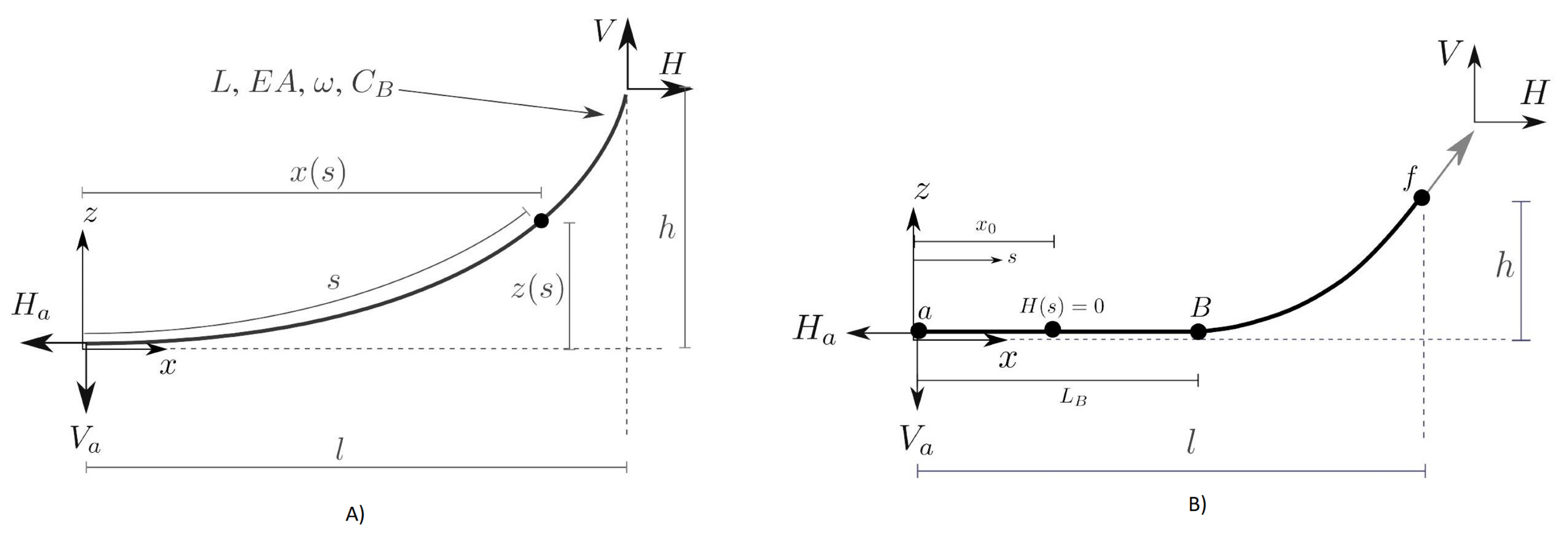
Subsequently, the catenary equations are simultaneously solved to find the horizontal and vertical fairlead forces for each line used to calculate the tension at the fairlead. As previously written, there are two type of catenary equations:

• Free–Hanging Line

  $$l=\frac{H}{\omega }+[ln(\frac{V}{H}+\sqrt{1+{\left(\frac{V}{H}\right)}^2})-ln(\frac{V-L\omega }{H}+\sqrt{1+{\left(\frac{V-L\omega }{H}\right)}^2})]+\frac{HL}{EA}$$

  (29)

  $$h=\frac{H}{\omega }+[\sqrt{1+{\left(\frac{V}{H}\right)}^2}-\sqrt{1+{\left(\frac{V-L\omega }{H}\right)}^2}]+\frac{1}{EA}\left(VL-\frac{L^2\omega }{2}\right)$$

  (30)

  $$\omega =gA\left({\rho }_{cable}-\rho \right)$$

  (31)
• Line Touching the Bottom

  $$l=L_B+\frac{H}{\omega }[ln(\frac{V}{H}+\sqrt{1+{\left(\frac{V}{H}\right)}^2})]+\frac{HL}{EA}+\frac{C_B\omega }{2EA}\left[x_0\lambda -L_B^2\right]$$

  (32)

  $$h=\frac{H}{\omega }[\sqrt{1+{\left(\frac{V}{H}\right)}^2}-1]+\frac{V^2}{2EA\omega }$$

  (33)

  $$\lambda =\left\{\begin{array}{cc}{L}_B-\frac{H}{C_B\omega }\hfill & x_0>0\hfill \\ 0\hfill & otherwise\hfill \end{array}\right.$$

  (34)

where:

• H: Horizontal fairlead force (Figure 5);
• V: Vertical fairlead force (Figure 5);
• A: Cable cross-section line;
• E: Young’s modulus;
• g: Gravity acceleration;
• ${\rho }_{cable}$: Cable density;
• $\rho$: Fluid density;
• L: Unstretched line length;
• $L_B$: Line length resting on the seabed (Figure 5B);
• $C_B$: Seabed friction coefficient;
• $x_0$: Horizontal force transition point (Figure 5B).

Finally, the force-balance equations for each node are solved to check the convergence:

$${\displaystyle F_x^j=\sum _{i=1}^N{H}_{i}cos{\alpha }_i-F{x}_j^{ext}=0}$$

(35)

$${\displaystyle F_y^j=\sum _{i=1}^N{H}_{i}sin{\alpha }_i-F{y}_j^{ext}=0}$$

(36)

$${\displaystyle F_z^j=\sum _{i=1}^N{V}_i-F{z}_j^{ext}+M_{j}g-g{B}_j\rho =0}$$

(37)

where:

• N: Elements i at node j
• $M_j$: Point mass applied to the node jth. Used to evaluate the clump weight;
• $B_j$: Displaced volume applied to node jth;
• $F^{ext}$: external force applied to node jth;
• ${\alpha }_i$: Angle between ith angle and global X direction.

The triad of forces described previously produces moments on the structure, because they have an arm described by the position vector ${\mathit{C}}_{\mathit{rot}}^{\mathbf{\prime }}$ (Equation (28)) of connection point $C^{\prime }$ on the rotated platform surface in the LSA reference frame. MAP++ does not calculate these moments, to do this the cross product between the tension vector and the position vector is made manually:

$${\mathit{M}}_{\mathit{C}}={\mathit{C}}_{\mathit{rot}}^{\mathbf{\prime }}\times {\mathit{T}}_{\mathit{C}}$$

(38)

The contributions of generalized loads coming from all the six mooring lines are then summed, and their sign changed to obtain the overall reaction exerted by the mooring lines on the floater.

2.4. Aerodynamics

The U.S. Department of Energy’s (DOE’s) and the Wind Department of the National Renewable Energy Laboratory’s (NREL) (website: https://www.nrel.gov/wind/) have developed a standardized wind turbine for usage in several different investigations, named NREL offshore 5-MW baseline wind turbine [44].

2.4.1. Wind-Speed Profile

The wind speed profile is highly influenced by geostrophic wind, surface roughness, Coriolis effects and thermal effects. For sufficiently stable atmospheric conditions, the wind-speed profile may be represented by a logarithmic or power law profile. As suggested by Jonkman [45], the power law expression was assumed to scale the wind speed value $U_H$ from the reference elevation of H = 10 m above the SWL of the site data to the 90 m of the hub.

$$U\left(z\right)=U_H{\left(\frac{z}{H}\right)}^{\alpha }$$

(39)

where the shear exponent $\alpha$, depending on the water surface roughness, for offshore wind turbines is given by IEC 61400-3 [46] as $\alpha =0.14$.

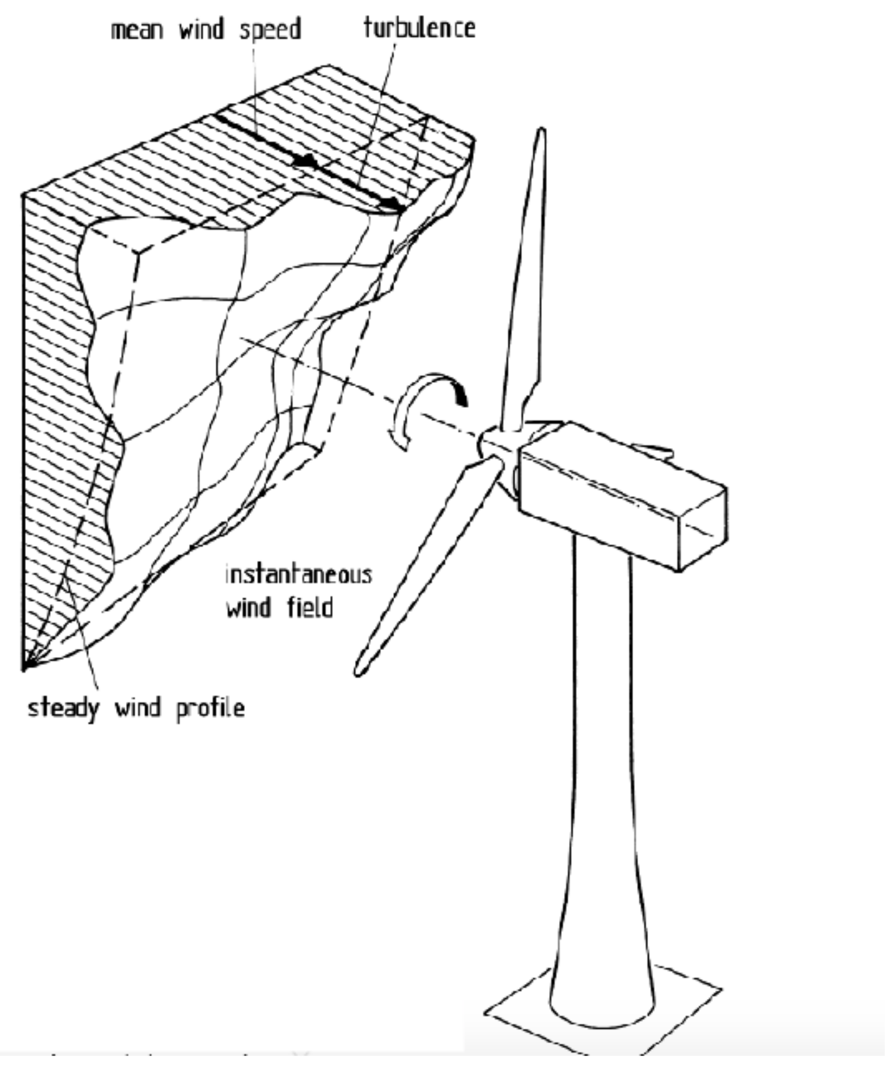
Turbulence

The short-term fluctuations in wind speed, in the order of tens to hundreds, are known as turbulence. Turbulence is a complex chaotic process and therefore its representation implies the use of statistical properties. If $\sigma$ is the standard deviation of wind speed about the mean wind speed $\overline{U}$, the level of turbulence is defined as:

$$I=\frac{\sigma }{\overline{U}}$$

(40)

The standard deviation $\sigma$ is roughly constant with height, so, since the mean wind speed $\overline{U}$ increases with height, the turbulence intensity I decreases with height. The IEC 61400-3 standard [46] recommends for the longitudinal direction:

$$I=I_{ref}\left(0.75+\frac{5.6}{\overline{U}}\right)$$

(41)

where $I_{ref}=$ 0.16, 0.14 or 0.12 depending on IEC classification of winds -‘A’, ‘B’, ‘C’- with A being the most intense.

“There are basically two methods for determining wind turbulence by theoretical means. One is via the energy spectrum of the turbulence, the other is by means of an actual wind speed time history. Independently of the chosen method, one phenomenon affecting the reaction of the wind rotor to turbulence must not be overlooked. In the open atmosphere, wind speed and turbulence are always unevenly distributed in space over the rotor-swept area. Many gusts strike the rotor not as a whole, but only on one side or only partially. This fact is significant for the response of the structure as regards the rotating rotor. The rotor blades "beat" into the gusts, i.e., the local wind speed changes, at their tangential speed. An observer travelling with the rotor blade experiences these speed changes considerably more strongly than he would in the steady-state system. Moreover, depending on the duration of the gust and the speed of the rotor, the rotor blade can encounter the same gust several times”

[47] (Figure 6).

In this study, through the Turbsim software [48], it is possible to add turbulence to the wind spectrum.

2.4.2. Shaft Torque Balance

The shafts are described as a one DOF system with no stiffness and no damping. The equation of rotation for the low-speed and high-speed shaft are respectively:

$$T_{rot}-T_{dt,rot}=I_{rot}\dot{\mathsf{\Omega }}$$

(42)

$$T_{dt,gen}-T_{gen}=I_{gen}{\dot{\mathsf{\Omega }}}_{gen}$$

(43)

where $T_{rot}$ is the rotor torque, $T_{gen}$ the generator torque, $T_{dt,rot}$ the torque transmitted by the gearbox to the rotor shaft, $T_{dt,gen}$ the torque transmitted by the gearbox to the generator shaft, $I_{rot}$ the rotor overall moment of inertia, $I_{gen}$ the generator moment of inertia, $\mathsf{\Omega }$ the rotor speed and ${\mathsf{\Omega }}_{gen}$ the generator speed. The moment of inertia of the rotor is the sum of the moment of inertia of the hub $I_{hub}$ and those of the three blades $I_{blade}$:

$$I_{rot}=I_{hub}+3I_{blade}$$

(44)

The gearbox ratio $N=97$ ties the speeds and torques between the two shafts through ${\mathsf{\Omega }}_{gen}/\mathsf{\Omega }=T_{dt,rot}/T_{dt,gen}=N$, then Equations (42) and (43) become:

$$T_{rot}-N{T}_{gen}=(I_{rot}+N^2{I}_{gen})\dot{\mathsf{\Omega }}=I_{dt}\dot{\mathsf{\Omega }}$$

(45)

where $I_{dt}=(I_{rot}+N^2{I}_{gen})=5.06\times {10}^9$ kgm${}^2$ is the moment of inertia of the transmission chain cast to the rotor shaft.

2.4.3. Aerodynamic Loads

The steady Blade Element Momentum (BEM), developed by Glauert [49] in 1935, is the most used method for calculating the velocities and the loads acting on a wind turbine rotor for any set of wind speed, rotor speed, pitch angle and turbine orientation [50,51,52]. This model originates from the union of two theories:

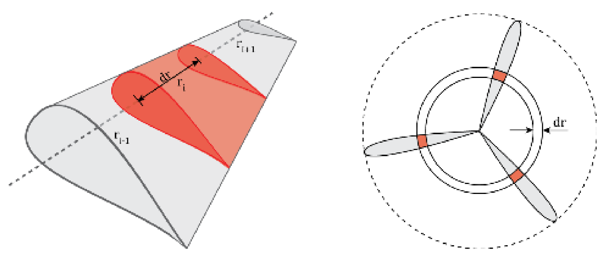
• blades are divided into small elements represented by 2D airfoils which are only subject to local physical events (blade element model); this means that all blade sections are independent and any spanwise evolution is neglected. The rotor disk area is divided into annuli of thickness dr; in each annulus there are Z blade elements of length dr, where Z is the number of wind turbine blades (Figure 7). The forces contribution from all annuli are summed along the span of the blade to calculate the total loads on the rotor.
• the rotor acts as an actuator disk (momentum theory) removing kinetic energy from the wind and thus gradually slowing down the stream, making the streamlines diverge; the disk is considered frictionless and the flow stationary, incompressible and frictionless; the momentum loss in the rotor plane is used to calculate the axial tangential velocities, that affect the forces calculated from the blade element theory.

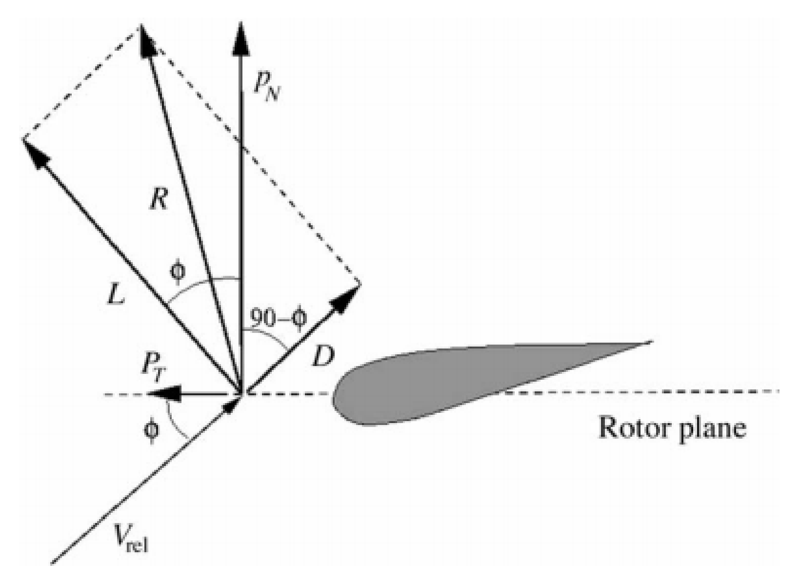
Assuming a 2D approach implies that there is no difference at all along the radial distance of a blade, i.e., that blade has an infinite span. The cross section of a blade, an airfoil, divides the incoming air into two streams, which are forced to follow the curved geometry. As the direction of the momentum of a particle varies following the stream, a pressure gradient $\partial p/\partial r=\rho V^2/r>0$ establishes from the lower to the upper surface, and since the pressure must be null far from the airfoil, this introduces a pressure drop. The resulting set of generalized forces are the lift L, perpendicular to the direction of the undisturbed wind velocity $V_0$, carrying the effect of the pressure difference, the drag D, parallel to $V_0$, carries the effect of the friction caused by the air, and a moment M, all conventionally applied at $1/4$ of the length of the chord c and expressed as generalized forces per unit of length. The set of loads acting on a blade airfoil are represented in Figure 8.

Being the wind resource associated with an available mechanical power $P_{avail}=\frac{1}{2}\dot{m}{V}_0^2=\frac{1}{2}\rho A{V}_0^3$ (where $\rho$ is the air density, A the rotor swept area and $\dot{m}$ the air flow rate) the set of generalized forces just introduced may be expressed by three dimensionless coefficients by normalizing them with respect to a measure of the available wind force:

$$\begin{array}{cc}\hfill & C_l=\frac{L}{\frac{1}{2}\rho V_0^{2}c}\mathrm{lift}\mathrm{coefficient}\hfill \end{array}$$

(46)

$$\begin{array}{cc}\hfill & C_d=\frac{D}{\frac{1}{2}\rho V_0^{2}c}\mathrm{drag}\mathrm{coefficient}\hfill \end{array}$$

(47)

$$\begin{array}{cc}\hfill & C_m=\frac{M}{\frac{1}{2}\rho V_0^2{c}^2}\mathrm{moment}\mathrm{coefficient}\hfill \end{array}$$

(48)

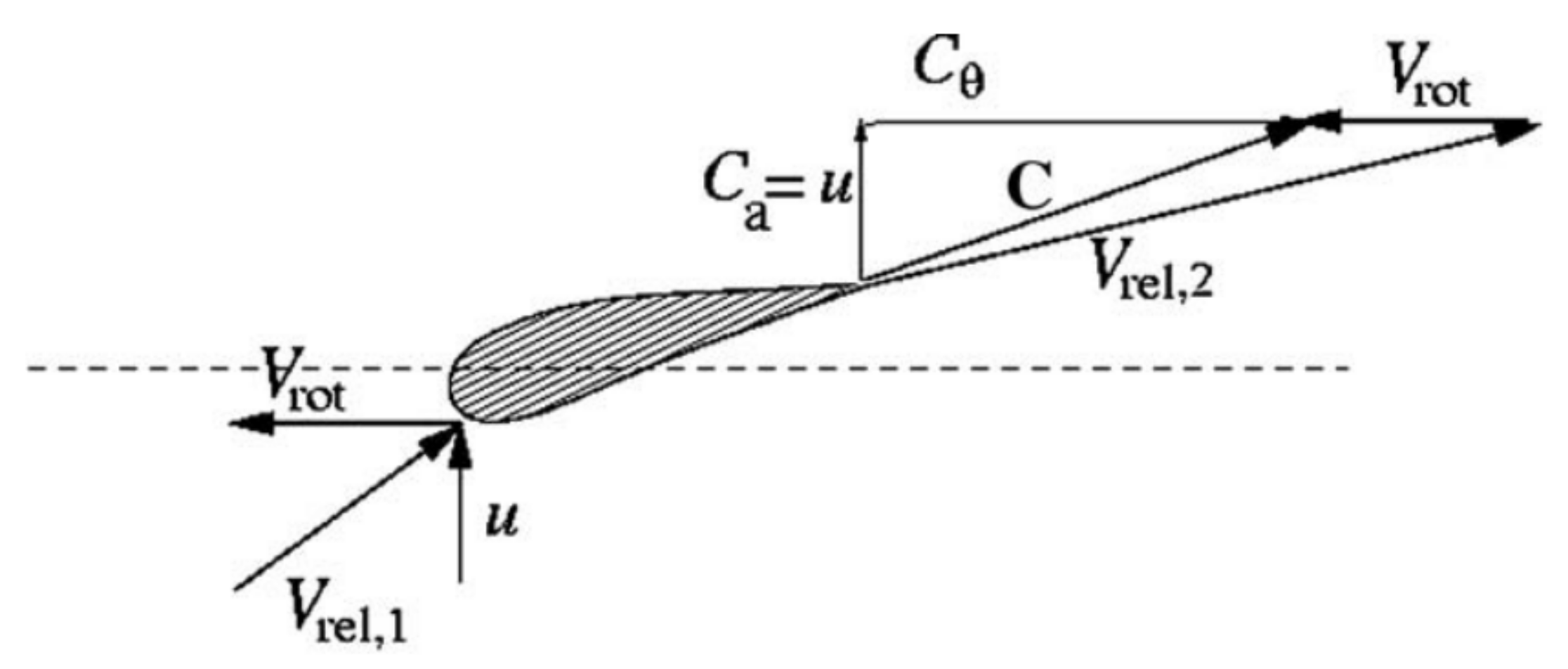
An airfoil is fully defined by the tables $C_l\left(\alpha \right),C_d\left(\alpha \right)$, where $\alpha$ is the angle of attack. In the reality, a blade cannot be considered as 2D. The first and most important effect of the spanwise variable geometry of a blade is the presence of tips, which introduce a discontinuity that causes as ultimate effect a complex system of trailing free vortices, which develops as if the rotor was also translating in the axial direction, thus describing a helical path. This may be explained in a simple manner considering it as a reaction for the extraction of a torque by the wind turbine, the air downstream must rotate in a direction opposite to that of the rotor. The effect of trailing vortices on the aerodynamic of the blade is the introduction of two orthogonal components of induced velocity: an axial induced velocity $a{V}_0$, opposite to the direction of the wind, and a tangential induced velocity $2a^{\prime }\mathsf{\Omega }r$, where a and $a^{\prime }$ are the axial and tangential induction factors and $\mathsf{\Omega }$ the rotor speed. Since the air has tangential component $2a^{\prime }\omega r$ downstream and null upstream, then at the rotor it may be considered as $a^{\prime }\mathsf{\Omega }r$. The velocity triangle at the rotor is then defined (Figure 9):

$$\begin{array}{cc}\hfill & V_a=(1-a)V_x\hfill \end{array}$$

(49)

$$\begin{array}{cc}\hfill & V_{rot}=(1+a^{\prime })V_y\hfill \end{array}$$

(50)

$$\begin{array}{cc}\hfill & {\mathit{V}}_{\mathit{rel}}={\mathit{V}}_{\mathit{a}}+{\mathit{V}}_{\mathit{rot}}\hfill \end{array}$$

(51)

From the momentum theory, the axial and tangential induction factors are respectively:

$$\begin{array}{cc}\hfill & a=\frac{1}{{\displaystyle \frac{4{sin}^2\varphi }{\sigma C_n}}+1}\hfill \end{array}$$

(52)

$$\begin{array}{cc}\hfill & a^{\prime }=\frac{1}{{\displaystyle \frac{4sin\varphi cos\varphi }{\sigma C_t}}-1}\hfill \end{array}$$

(53)

where the local solidity $\sigma$ is defined as the actual fraction of circumference covered by blades:

$$\sigma =\frac{Bc}{2\pi r}$$

(54)

An iterative algorithm is used to determine the convergence values of a and $a^{\prime }$ and thus determine L and D. As an initial approximation [54], the induction factors may be assumed as:

$$a_0=\frac{1}{4}\left[2+\pi {\lambda }_r\sigma -\sqrt{4-4\pi {\lambda }_r\sigma +\pi {\lambda }_r^2\sigma (8\theta +\pi \sigma )}\right]$$

(55)

where ${\lambda }_r=\mathsf{\Omega }r/V_0$ is the tip-speed ratio, and

$$a_0^{\prime }=0$$

(56)

Since the aerodynamic coefficients $C_l$ and $C_d$ used in the blade element theory depend on the angle of attack $\alpha$ of the inflow, the latter must be determined as:

$$\alpha =\varphi -\theta$$

(57)

where $\theta =\beta +{\theta }_p$ is the local pitch of the blade, sum of the twist angle $\beta$ and the active pitch control angle ${\theta }_p$, and $\varphi$ is the angle between the plane of rotation and the relative velocity $V_{rel}$, given by:

$$tan\varphi =\frac{V_a}{V_{rot}}=\frac{(1-a)V_x}{(1+a^{\prime })V_y}$$

(58)

Considering an annulus of width $dr$, from the blade element theory the normal and tangential contributions $p_n$ and $p_t$ are related to the lift and drag forces L and D through the geometric relations:

$$\begin{array}{cc}\hfill & p_n=Lcos\varphi +Dsin\varphi \hfill \end{array}$$

(59)

$$\begin{array}{cc}\hfill & p_t=Lsin\varphi -Dcos\varphi \hfill \end{array}$$

(60)

which, normalized with respect to the inflow representative force $\frac{1}{2}\rho V_0^{2}c$, become, according to the definitions Equations (46) and (47):

$$\begin{array}{cc}\hfill & C_n=C_l\left(\alpha \right)cos\varphi +C_d\left(\alpha \right)sin\varphi \hfill \end{array}$$

(61)

$$\begin{array}{cc}\hfill & C_t=C_l\left(\alpha \right)sin\varphi -C_d\left(\alpha \right)cos\varphi \hfill \end{array}$$

(62)

The definitive algorithm will be presented after all the corrections to the BEM model.

Corrections to the BEM Model

One can easily notice that many limitations affect the simple BEM model. To overcome some of these, the following corrections are implemented:

• Prandtl’s tip-loss factor: considers that the airflow is not parallel near the tip of the blade.
• Glauert correction: in reality the thrust force on the turbine will not decrease when $a>0.4$, but its value will increase beyond 1. It avoids overestimating the tangential load with turbulent wind.
• Skewed wake correction: considers the deflection of the inflow wind that increases the induction factor; in fact, the wind direction is not perpendicular to the plane of rotation of the blades.

BEM Model Algorithm

The definitive BEM model algorithm is summarized here.

• Discretize the blade into $n_{nodes}$ nodes, each i-th node of length $l_{BE,i}$ representing the blade element in that section
• Find the loads for each node, through the following steps (BEM theory):

  (a)

  Estimate the starting values of axial and tangential induction factor and flow angle by mean of Equations (55) and (56), with a starting flow angle ${\varphi }_0=0$.

  (b)

  Iteration cycle for convergence of the induction factors, which provides:

  • Calculate the angle of attack by mean of Equation (57).

    $$\alpha ={\varphi }_0-(\beta +{\theta }_p)$$
  • Read the lift and drag coefficients from airfoil tables for $\alpha$

    $$\begin{array}{cc}\hfill & C_l=C_l\left(\alpha \right)\hfill \\ \hfill & C_d=C_d\left(\alpha \right)\hfill \end{array}$$
  • Calculate normal and tangential forces coefficients by mean of Equations (61) and (62).

    $$\begin{array}{cc}\hfill & C_n=C_l\left(\alpha \right)cos{\varphi }_0+C_d\left(\alpha \right)sin{\varphi }_0\hfill \end{array}$$

    $$\begin{array}{cc}\hfill & C_t=C_l\left(\alpha \right)sin{\varphi }_0-C_d\left(\alpha \right)cos{\varphi }_0\hfill \end{array}$$
  • Calculate Prantdtl’s tip- and hub-loss factor

    $$F_{Pr}\left(r\right)=F_{Pr,tip}\left(r\right)·F_{Pr,hub}\left(r\right)$$

    (63)

    $$\begin{array}{cc}\hfill & F_{Pr,tip}\left(r\right)=\frac{2}{\pi }{cos}^{-1}\left(e^{-{\displaystyle \frac{B}{2}}{\displaystyle \frac{R-r}{rsin{\varphi }_0}}}\right)\hfill \end{array}$$

    (64)

    $$\begin{array}{cc}\hfill & F_{Pr,hub}\left(r\right)=\frac{2}{\pi }{cos}^{-1}\left(e^{-{\displaystyle \frac{B}{2}}{\displaystyle \frac{r-R_h}{rsin{\varphi }_0}}}\right)\hfill \end{array}$$

    (65)
  • Calculate the axial and tangential induction factor using Glauert correction:

    $$\begin{array}{cc}\hfill & a=\left\{\begin{array}{cc}{\displaystyle \frac{\kappa }{\kappa +1}}\hfill & \hfill {\varphi }_0>0,\kappa \le \frac{2}{3}\\ {\displaystyle \frac{{\gamma }_1-\sqrt{{\gamma }_2}}{{\gamma }_3}}\hfill & \hfill {\varphi }_0>0,\kappa >\frac{2}{3},{\gamma }_3\ne 0\\ 1-{\displaystyle \frac{1}{2\sqrt{{\gamma }_2}}}\hfill & \hfill {\varphi }_0>0,\kappa >\frac{2}{3},{\gamma }_3=0\\ {\displaystyle \frac{\kappa }{\kappa -1}}\hfill & \hfill {\varphi }_0<0,\kappa >1\\ 0\hfill & \hfill {\varphi }_0<0,\kappa \le 1\end{array}\right.\hfill \end{array}$$

    (66)

    $$\begin{array}{cc}\hfill & a^{\prime }={\displaystyle \frac{{\kappa }^{\prime }}{1-{\kappa }^{\prime }}}\hfill \end{array}$$

    (67)

    where

    $$\kappa =\frac{\sigma C_n}{4F_{Pr}{sin}^2{\varphi }_0};{\kappa }^{\prime }=\frac{\sigma C_t}{4F_{Pr}sin{\varphi }_{0}cos{\varphi }_0}$$

    (68)

    and

    $$\left\{\begin{array}{c}{\gamma }_1=2F_{Pr}\kappa -\left(\frac{10}{9}-F_{Pr}\right)\hfill \\ {\gamma }_2=2F_{Pr}\kappa -F_{Pr}\left(\frac{4}{3}-F_{Pr}\right)\hfill \\ {\gamma }_3=2F_{Pr}\kappa -\left(\frac{25}{9}-2F_{Pr}\right)\hfill \end{array}\right.$$

    (69)
  • Calculate the flow angle by mean of Equation (58).
  • Check for convergence on the flow angle ($\epsilon$ is an arbitrary tolerance)

    $$|\varphi -{\varphi }_0|<\epsilon$$

    (70)
  • If the cycle has not converged yet, use the values a, $a^{\prime }$ and ${\varphi }_0=\varphi$ as new attempt values for the iteration, otherwise, continue. The relative tolerance for convergence is 0.01${}^{\circ }$ and a maximum number of iterations is 1000.

  (c)

  Once the values of a and $a^{\prime }$ are obtained, skew correction is applied on a:

  $$a_{skew}=a\left(1+\frac{15\pi }{64}\frac{r}{R}tan\frac{\chi }{2}sin\psi \right)$$

  (71)

  where

  $$\chi =(0.6a+1){\chi }_0$$

  (72)

  and, considering $V_{Avg}$ the relative velocity (wind minus structure) averaged over the rotor disk:

  $${\chi }_0=\frac{V_{Avg,x}}{\sqrt{V_{Avg,x}^2+V_{Avg,y}^2+V_{Avg,z}^2}}$$

  (73)

  (d)

  Calculate the relative wind speed by Equation (51).

  (e)

  Calculate the normal and tangential loads per unit length

  $$\begin{array}{cc}\hfill & p_n=\frac{1}{2}\rho C_n{V}_{rel}^{2}c\hfill \end{array}$$

  (74)

  $$\begin{array}{cc}\hfill & p_t=\frac{1}{2}\rho C_t{V}_{rel}^{2}c\hfill \end{array}$$

  (75)

• Calculate the aerodynamic loads at the nacelle as the integral of the normal and tangential loads over the length of each of the 3 blades, defined r the node position between hub radius $r_h$ and the blade length $r_b$

  $$\begin{array}{cc}\hfill & F{x}_{aer}={\int }_{r_h}^{r_b}{p}_{n,1}dr+{\int }_{r_h}^{r_b}{p}_{n,2}dr+{\int }_{r_h}^{r_b}{p}_{n,3}dr\hfill \end{array}$$

  (76)

  $$\begin{array}{cc}\hfill & F{y}_{aer}={\int }_{r_h}^{r_b}{p}_{t,1}sin{\psi }_{1}dr+{\int }_{r_h}^{r_b}{p}_{t,2}sin{\psi }_{2}dr+{\int }_{r_h}^{r_b}{p}_{t,3}sin{\psi }_{3}dr\hfill \end{array}$$

  (77)

  $$\begin{array}{cc}\hfill & F{z}_{aer}={\int }_{r_h}^{r_b}{p}_{t,1}cos{\psi }_{1}dr+{\int }_{r_h}^{r_b}{p}_{t,2}cos{\psi }_{2}dr+{\int }_{r_h}^{r_b}{p}_{t,3}cos{\psi }_{3}dr\hfill \end{array}$$

  (78)

  $$\begin{array}{cc}\hfill & M{x}_{aer}={\int }_{r_h}^{r_b}{p}_{t,1}rdr+{\int }_{r_h}^{r_b}{p}_{t,2}rdr+{\int }_{r_h}^{r_b}{p}_{t,3}rdr\hfill \end{array}$$

  (79)

  $$\begin{array}{cc}\hfill & M{y}_{aer}={\int }_{r_h}^{r_b}{p}_{n,1}rsin{\psi }_{1}dr+{\int }_{r_h}^{r_b}{p}_{n,2}rsin{\psi }_{2}dr+{\int }_{r_h}^{r_b}{p}_{n,3}rsin{\psi }_{3}dr\hfill \end{array}$$

  (80)

  $$\begin{array}{cc}\hfill & M{z}_{aer}={\int }_{r_h}^{r_b}{p}_{n,1}rcos{\psi }_{1}dr+{\int }_{r_h}^{r_b}{p}_{n,2}rcos{\psi }_{2}dr+{\int }_{r_h}^{r_b}{p}_{n,3}rcos{\psi }_{3}dr\hfill \end{array}$$

  (81)

It is worth highlighting that the inflow wind speed considered for computations is the sum of the absolute wind speed and the relative motion of the rotor, resulting from the rigid translation of the system and the fore-aft motion around the COG. Once the loads on the nacelle ${\mathit{F}}_{\mathit{aer}}$ have been obtained, they are transported to the tower base obtaining ${\mathit{F}}_{\mathit{wt}}$.

2.4.4. Control System

The control system chosen for the NREL 5-MW wind turbine was a conventional variable-speed, variable pitch-to-feather configuration [44]. It is made up of two control systems, working independently:

• A generator-torque controller is designed to maximize the power extraction below the nominal point
• A full-span rotor-collective blade-pitch controller is designed to regulate generator speed above the nominal point

The nominal or rated point is defined as the reference operation point for the maximum continuous power conversion, towards which the control system tends. It is summarized in

Table 3. Rated operation point for the wind turbine.

rated wind speed	11.4	m/s
rated rotor speed	12.1	rpm
rated generator speed	1173.7	rpm
rated generator torque	43,094	Nm
rated mechanical power	5.30	MW
rated electric power	5.00	MW

.

This work does not include any further control for start-up, shutdown, safety and protection sequences or any nacelle-yaw regulation.

Generator-Torque Controller

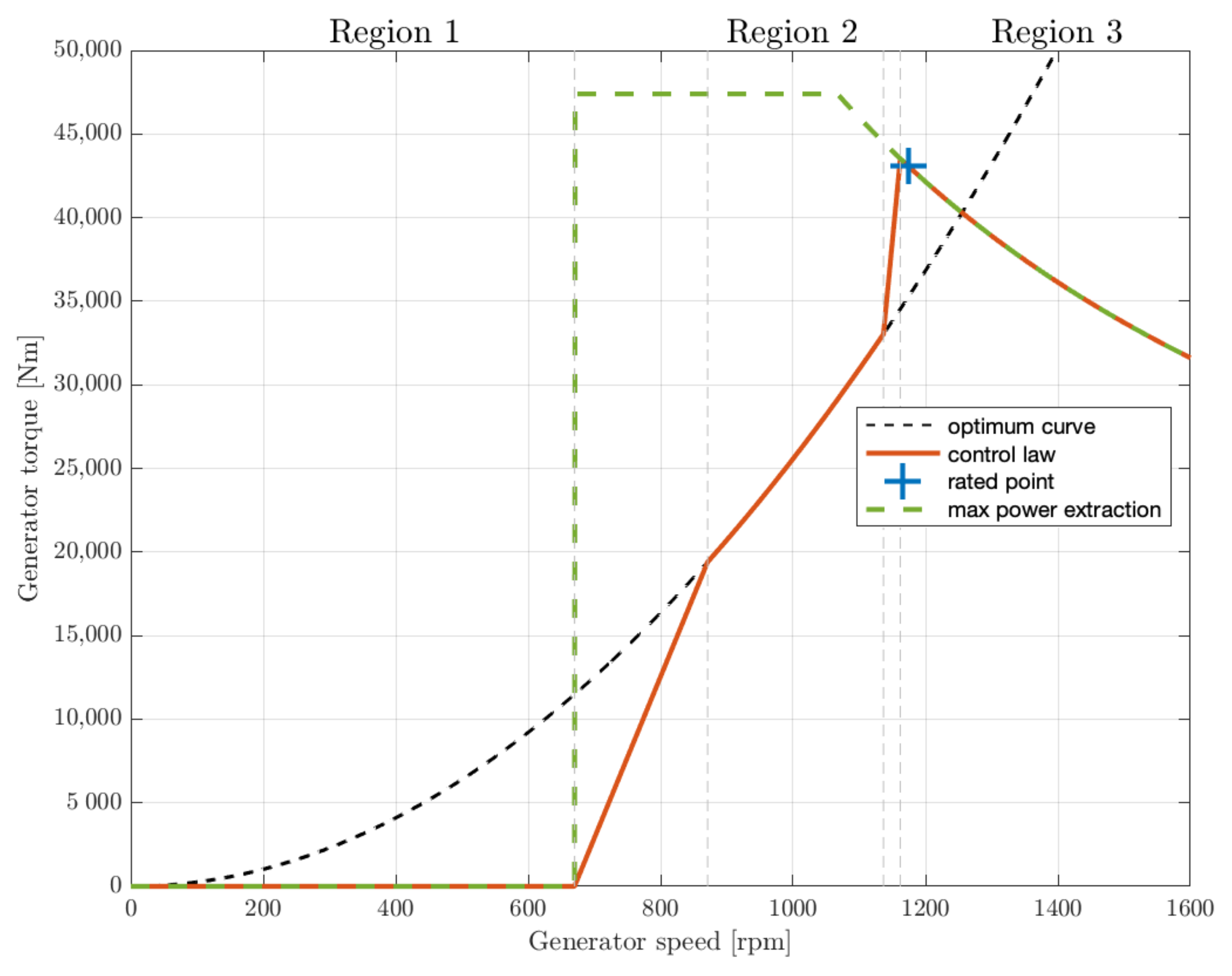
The generator-torque control law is designed to have three main regions and two transition regions in-between. Before describing this mapping, it is worth reminding that, while the torque originated by wind acts as an accelerating load, the generator torque, converting mechanical energy to electrical energy, acts as a braking load, and an equilibrium has to be sought between them for the sake of regularity. The control law is described in the next lines and plotted in Figure 10.

The generator torque is computed as a tabulated function of the filtered generator speed, incorporating five control regions: 1, 1${}_2^1$, 2, 2${}_2^1$, and 3.

Region 1 is a control region before cut-in wind speed, where the generator is detached from the rotor so as to allow the wind to accelerate the rotor for start-up. In this region, the generator torque is zero and no power is extracted from the wind.

Region 2 is a control region for optimizing power capture. Here, to maintain the tip speed ratio constant at its optimal value, the generator torque is proportional to the square of the filtered generator speed $T_{gen}=k_{opt}{\mathsf{\Omega }}_{gen}^2$.

In Region 3 is the constant power region, where the generator torque is inversely proportional to the filtered generator speed. Therefore, by increasing the generator speed beyond the rated value ${\mathsf{\Omega }}_{gen,rated}$ = 1173 rpm, the torque will drop below the rated value $T_{gen,rated}$ = 43,093 Nm.

Region 1$\frac{\mathit{1}}{\mathit{2}}$ is the start-up region, a linear transition between Regions 1 and 2. This region is used to place a lower limit on the generator speed to limit the wind turbine’s operational speed range and is defined in the region of generator speed between 670 rpm and 30% above this value (or 871 rpm).

Region 2$\frac{\mathit{1}}{\mathit{2}}$ is a linear transition between Regions 2 and 3 with a torque slope corresponding to the slope of an induction machine (10% in our case). Region 2$\frac{\mathit{1}}{\mathit{2}}$ is typically needed to limit tip speed (and hence noise emissions) at rated power. The boundaries of this region are the optimum power extraction curve of Region 2 and the constant power curve of Region 3, intersected at 99% of the rated generator speed, or 1162 rpm [44].

This control system does not include any control loop for the high-speed shaft rotation because the drivetrain inner structural damping is considered sufficient to filter any torsional vibration.

There is, however, a conditional statement (green curve in Figure 10) on the generator-torque controller so that the torque would follow the constant power curve (as if it was in Region 3)—regardless of the generator speed—whenever the previous blade-pitch-angle command was 1${}^{\circ }$ or greater [44]. Since the blade-pitch-angle control intervenes when the generator speed is greater than the nominal value, bringing it back below this value, there is a transient in which the generator speed is already below the nominal value, while the blade-pitch-angle has not yet returned to zero. In this situation, the constant power curve is followed to optimize the extracted power. This results in improved output power quality (fewer dips below rated) and quantity (tests show a 5% increase of the extracted power) at the expense of short-term overloading of the generator and the gearbox: for this reason, the torque is saturated to a maximum of 10% above rated, or 47,403 Nm, to avoid this excessive overloading.

Finally, a torque rate limit of 15,000 Nm/s has been imposed. In Region 3, where the generator speed is above the rated value, the blade-pitch control system is active.

Blade-Pitch Controller

As anticipated in Generator-Torque Controller, the full-span rotor-collective blade-pitch-angle regulates the generator speed in Region 3 (where it exceeds its rated speed of 1173 rpm) to maintain it at its rated value through a proportional-integral control (PI), using variable gains [44,55].

Starting from Equation (45), by perturbing the rotor speed of an amount $\Delta \mathsf{\Omega }$ about the rated rotor speed ${\mathsf{\Omega }}_0$:

$$T_{rot}-N{T}_{gen}=I_{dt}\frac{d}{dt}({\mathsf{\Omega }}_0+\Delta \mathsf{\Omega })=I_{dt}\frac{d\Delta \mathsf{\Omega }}{dt}$$

(82)

In Region 3, the generator torque is regulated so to maintain a constant generator power:

$$T_{gen}\left({\mathsf{\Omega }}_{gen}\right)=\frac{P_0}{{\mathsf{\Omega }}_{gen}}=\frac{P_0}{N_{gear}\mathsf{\Omega }}$$

(83)

where $P_0$ is the rated mechanical power, while the rotor torque, assuming that it only varies with the blade pitch ${\theta }_p$ and not with the rotor speed $\mathsf{\Omega }$, is computed around the rated rotor speed ${\mathsf{\Omega }}_0$ as:

$$T_{rot}(\mathsf{\Omega },{\theta }_p)=\frac{P(\mathsf{\Omega },{\theta }_p)}{\mathsf{\Omega }}\simeq \frac{P\left({\theta }_p\right){|}_{\mathsf{\Omega }={\mathsf{\Omega }}_0}}{\mathsf{\Omega }}=T_{rot}\left({\theta }_p\right)$$

(84)

By expressing the first-order Taylor expansion of Equation (84) with respect to the blade pitch ${\theta }_p$, centered at the rated operating blade pitch ${\theta }_{p,0}$:

$$\begin{array}{cc}\hfill T_{rot}\left({\theta }_p\right)& \simeq T_{rot}\left({\theta }_p\right){|}_{{\theta }_p={\theta }_{p,0}}+\frac{d{T}_{rot}\left({\theta }_p\right)}{d{\theta }_p}{|}_{{\theta }_p={\theta }_{p,0}}({\theta }_p-{\theta }_{p,0})=\hfill \\ \hfill & =\frac{P\left({\theta }_p\right)}{{\mathsf{\Omega }}_0}{|}_{\begin{array}{c}{\theta }_p={\theta }_{p,0}\\ \mathsf{\Omega }={\mathsf{\Omega }}_0\end{array}}+\frac{1}{{\mathsf{\Omega }}_0}\frac{dP\left({\theta }_p\right)}{d{\theta }_p}{|}_{\begin{array}{c}{\theta }_p={\theta }_{p,0}\\ \mathsf{\Omega }={\mathsf{\Omega }}_0\end{array}}({\theta }_p-{\theta }_{p,0})=\hfill \\ \hfill & =\frac{P_0}{{\mathsf{\Omega }}_0}+\frac{1}{{\mathsf{\Omega }}_0}\frac{dP}{d{\theta }_p}\Delta {\theta }_p\hfill \end{array}$$

(85)

where $\Delta {\theta }_p$ represents a small perturbation of the blade pitch angle about its rated operating point ${\theta }_{p,0}$ (zero in this case). By expressing the blade-pitch regulation starting from the speed perturbation with a proportional-integrative control law (PI), it is possible to write:

$$\Delta {\theta }_p=K_P{N}_{gear}\Delta \mathsf{\Omega }+K_I{N}_{gear}{\int }_0^t\Delta \mathsf{\Omega }dt$$

(86)

where $K_P$ is the proportional gain and $K_I$ the integrative gain. As suggested by Jonkman [45], a derivative term is not implemented, as it would not improve the response of the system. By inserting equations Equations (84)–(86) into the equation of motion Equation (82), it is possible to obtain, defined $\Delta \mathsf{\Omega }=\dot{\phi }$:

$$\frac{P_0}{\mathsf{\Omega }}+\frac{1}{{\mathsf{\Omega }}_0}\frac{dP}{d{\theta }_p}\left(K_P{N}_{gear}\dot{\phi }+K_I{N}_{gear}\phi \right)-\frac{P_0}{\mathsf{\Omega }}=I_{dt}\ddot{\phi }$$

(87)

which can be rearranged as:

$$I_{dt}\ddot{\phi }+\left[-\frac{dP}{d{\theta }_p}\frac{N_{gear}{K}_P}{{\mathsf{\Omega }}_0}\right]\dot{\phi }+\left[-\frac{dP}{d{\theta }_p}\frac{N_{gear}{K}_P}{{\mathsf{\Omega }}_0}\right]\phi =0$$

(88)

that, in the canonical form:

$$M\ddot{\phi }+C\dot{\phi }+K\phi =0$$

(89)

defines the natural frequency and the damping ratio of the second order system:

$${\omega }_n=\sqrt{\frac{M}{K}}\zeta =\frac{C}{2M{\omega }_n}$$

(90)

A typical damping ratio for a control system is $0.7$, used to compensate for neglecting negative damping from the generator-torque controller in the determination of $K_P$, while the natural frequency suggested by Hansen [56] is 0.60 rad/s.

The two gains of the controller take the form:

$$\begin{array}{cc}\hfill K_P& ={\displaystyle \frac{2I_{dt}{\omega }_n\zeta {\mathsf{\Omega }}_0}{-N_{gear}{\displaystyle \frac{dP}{d{\theta }_p}}}}\hfill \end{array}$$

(91)

$$\begin{array}{cc}\hfill K_I& ={\displaystyle \frac{I_{dt}{\omega }_n^2{\mathsf{\Omega }}_0}{-N_{gear}{\displaystyle \frac{dP}{d{\theta }_p}}}}\hfill \end{array}$$

(92)

The pitch sensitivity $dP/d{\theta }_p$ is computed, as described by Jonkman, by “performing a linearization analysis at a number of given, steady, and uniform wind speeds at the rated rotor speed (${\mathsf{\Omega }}_0$ = 12.1 rpm) and at the corresponding blade-pitch angles that produce the rated mechanical power ($P_0$ = 5.297 MW). The linearization analysis involves perturbing the rotor-collective blade-pitch angle by a very small quantity at each operating point and measuring the resulting variation in aerodynamic power” [45]. The ratio $dP/d{\theta }_p$ varies nearly linearly with blade-pitch angle ${\theta }_p$:

$$\begin{array}{cc}\hfill \frac{dP}{d{\theta }_p}& ={\displaystyle \frac{{\displaystyle \frac{dP}{d{\theta }_p}}{|}_{{\theta }_p=0}}{{\theta }_{p,k}}}{\theta }_p+\frac{dP}{d{\theta }_p}{|}_{{\theta }_p}=\hfill \\ \hfill & ={\displaystyle \frac{dP}{d{\theta }_p}}{|}_{{\theta }_p=0}\left(1+{\displaystyle \frac{{\theta }_p}{{\theta }_{p,k}}}\right)\hfill \end{array}$$

(93)

where ${\theta }_{p,k}=$ 6.3${}^{\circ }$ is the blade-pitch angle at which the pitch sensitivity has doubled from its value at the rated operating point ${\theta }_p=0$. Then the PI gains become:

$$\begin{array}{cc}\hfill K_P\left({\theta }_p\right)& ={\displaystyle \frac{2I_{dt}{\omega }_n\zeta {\mathsf{\Omega }}_0}{-N_{gear}{\displaystyle \frac{dP}{d{\theta }_p}}}}GK\left({\theta }_p\right)\hfill \end{array}$$

(94)

$$\begin{array}{cc}\hfill K_I\left({\theta }_p\right)& ={\displaystyle \frac{I_{dt}{\omega }_n^2{\mathsf{\Omega }}_0}{-N_{gear}{\displaystyle \frac{dP}{d{\theta }_p}}}}GK\left({\theta }_p\right)\hfill \end{array}$$

(95)

where

$$GK\left({\theta }_p\right)={\displaystyle \frac{1}{1+{\displaystyle \frac{{\theta }_p}{{\theta }_{p,k}}}}}$$

(96)

Then, the values found for the gains at ${\theta }_p=0$, where $GK=0$, are:

$$\begin{array}{cc}\hfill K_P({\theta }_p=0)& =0.01882681\mathrm{s}\hfill \end{array}$$

(97)

$$\begin{array}{cc}\hfill K_I({\theta }_p=0)& =0.008068634\hfill \end{array}$$

(98)

3. Results

3.1. Choice of the Best Location

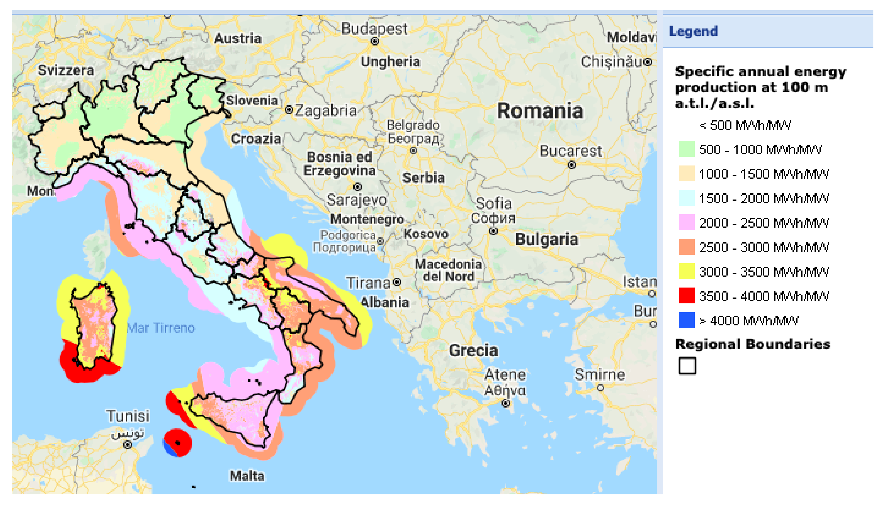
The research of the best installation site started from the map in Figure 11 showing specific productivity in each area of the Italian sea. As could be noted, the best locations are near Pantelleria island, in the middle of the Strait of Siciliy, and in the southern part of Sardinia.

By consulting the ERA5 ECMWF [58] database, hourly wind data for the last decade were obtained and then extracted using Qgis [59] software. Starting from the entire marine area within the Italian borders around Pantelleria, the best installation site has been identified through the following procedure: for each spot of the selected area the annual productivity was evaluated putting together wind distribution and the power curve of a NREL 5 MW reference wind turbine. Once the best spot was identified, a finer grid was built to identify the best site in that area. To make the right choice, in addition to productivity other parameters were considered (in order of importance):

• The distance from shore, that impacts on the installation costs (longer route for laying vessels) and visual pollution (the greater the distance from the coast, the less the wind farm will be visible).
• The sea depth, which should be considered for the mooring costs (shorter bathymetry means shorter length of the mooring lines).
• Air and sea traffic: the wind farm cannot be installed on routes traveled by ships or planes [60,61,62].
• Migration of birds: considered not to disturb the migration [63].
• Geo-political reasons. All other conditions being equal, areas not close to foreign borders are preferred.

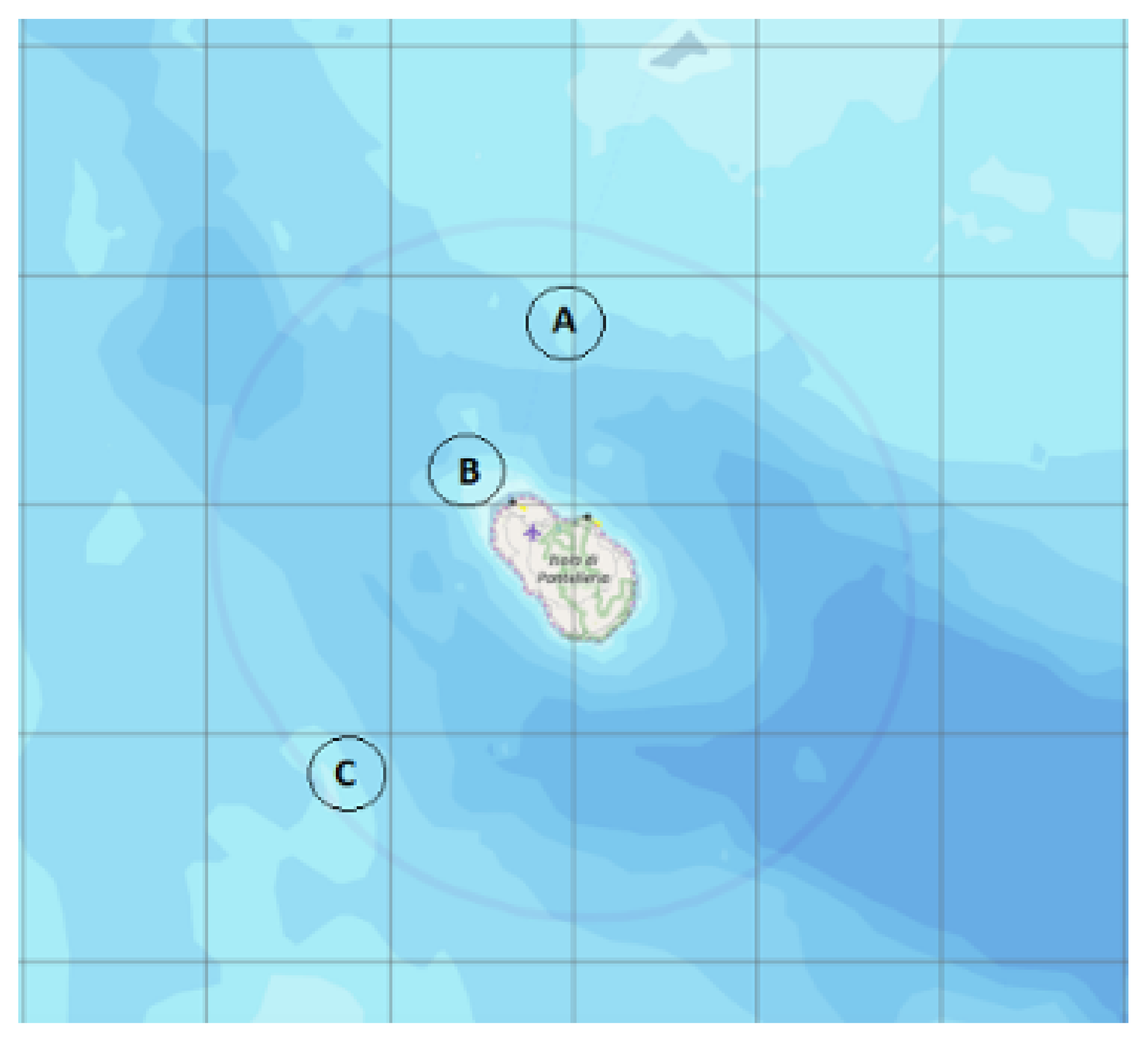
Combining all this parameters, three best sites were chosen (Figure 12). The characteristics of these site are described in

Table 4. Charateristics of study sites.

	Site A	Site B	Site C
Sea depth	120 m	420 m	115 m
Distance from shore	21.5 km	8.3 km	26.5 km
Productivity	4235 MWh/MW	4320 MWh/MW	4205 MWh/MW
C.F.	48.3%	49.3%	48.0%
Coordinates	LAT 37.01${}^{\circ }$ N, LONG 12.02${}^{\circ }$ E	LAT 36.54${}^{\circ }$ N, LONG 11.54${}^{\circ }$ E	LAT 36.37${}^{\circ }$ N, LONG 11.48${}^{\circ }$ E

.

Provided that Site B is very closed to the coast, reducing the advantages in terms of limited landscape impact, and that site C is very near to the border with Tunisia, site A was finally chosen for the hereby presented case study.

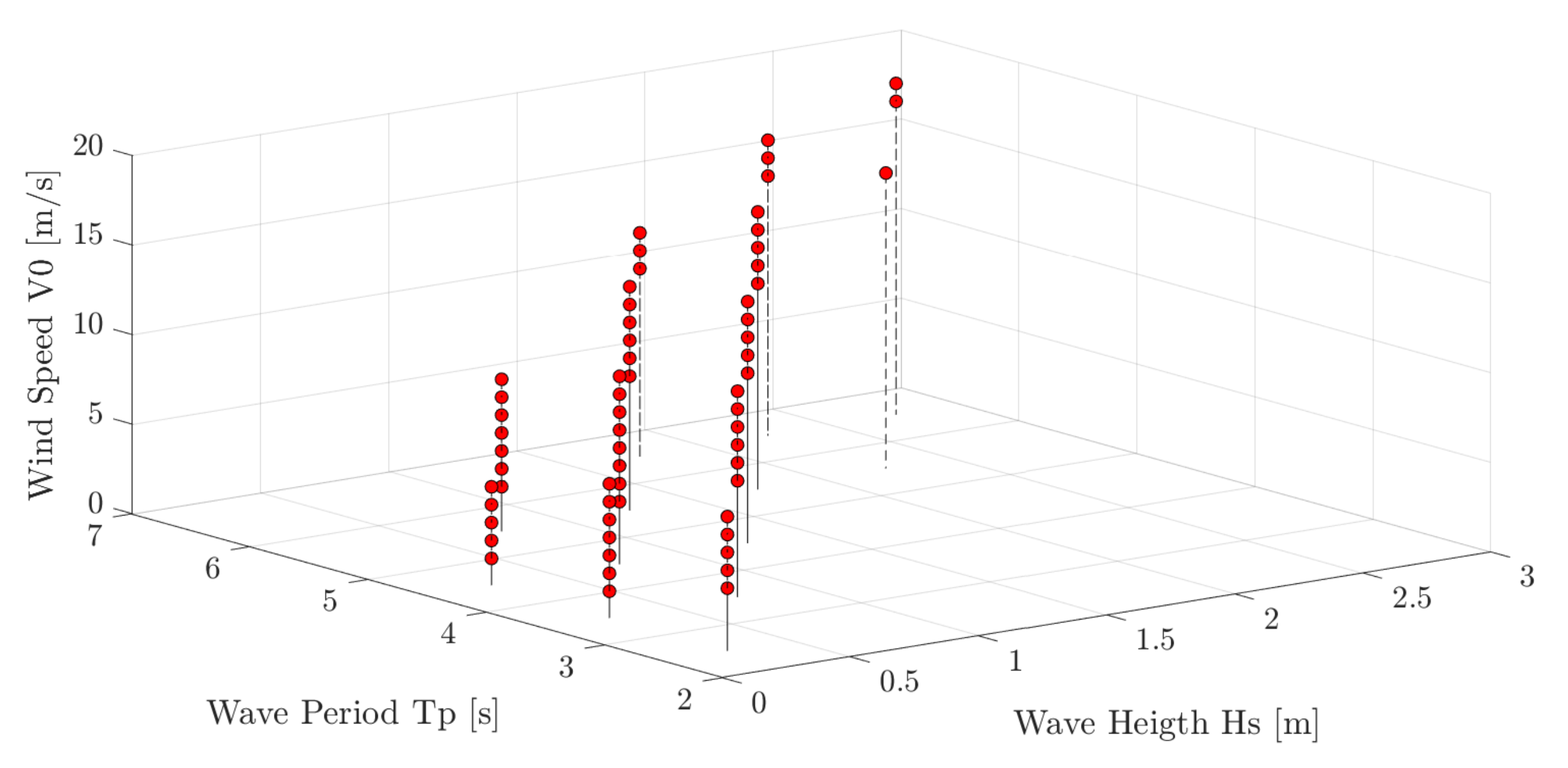
Once the site with the best wind resource was chosen, hourly marine data (height and wave period) of the last three years were downloaded from ERA5 ECMWF and extracted using software Qgis. Combining all the combinations of wave height $H_s$, wave period $T_p$ and wind speed $V_0$, triads were formed $(H_s,T_p,V_0)$, for a total of 26,280 records. Classes of belonging have therefore been defined, in order to detect the most frequent triads and then use them in simulations. From the $12\times 11\times 27=3564$ triads thus formed, those with a probability greater than 0.5% were selected (which together represent approximately 78% of the triads). The 63 triads thus obtained were then sorted in order of probability, so that simulation $n.1$ was the most probable. In this way it is possible to select the desired simulation by script through an identification index. Figure 13 represents the location of the 63 triads selected.

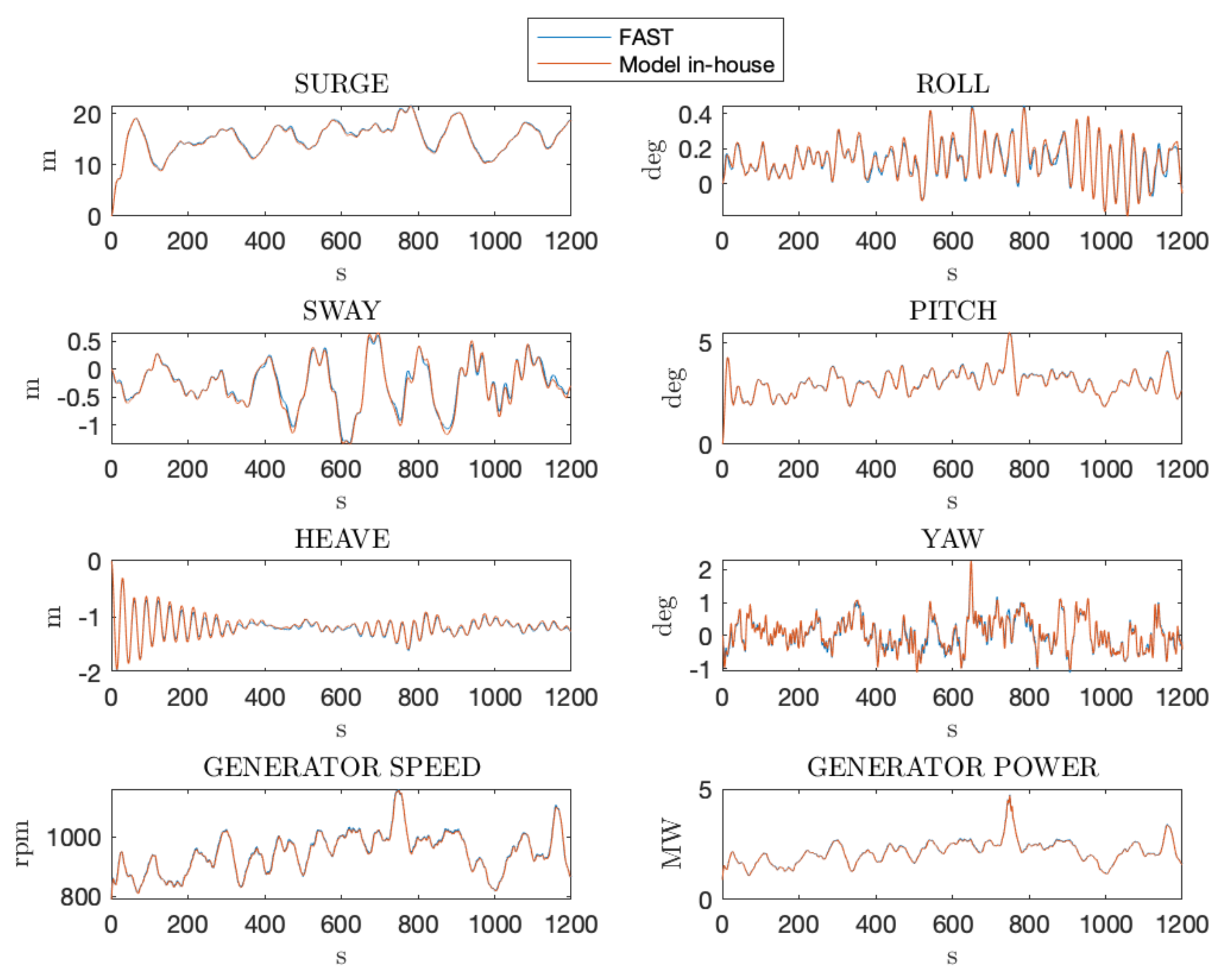
3.2. Comparison with FAST v8.16

Since FAST is the reference software for the simulation of offshore wind turbine, the results of the model created were compared with those of FAST. The choice to develop an in-house model on MATLAB is driven by the greater simplicity in setting the inputs and by a more intuitive structure: in FAST, in fact, the input files are inserted and the outputs are received without fully knowing the internal procedure. Furthermore, editing the input files is not trivial, requiring good programming knowledge. With the model created it is possible to modify the simulation parameters directly from the script, observing each step of the simulation and understanding the process of moving from inputs to outputs.

The in-house model manages to faithfully reproduce the FAST outcomes, resulting in RMSE (Root Mean Square Error) on position and output power lower than 2%. However, it has significant limitations such as the longer calculation time (about 5 minutes, almost the double of FAST) and the absence of elastic theory.

Figure 14 represents a particular graphic comparison of the 6 DOFs displacements, generator speed and generator power between the in-house model and FAST.

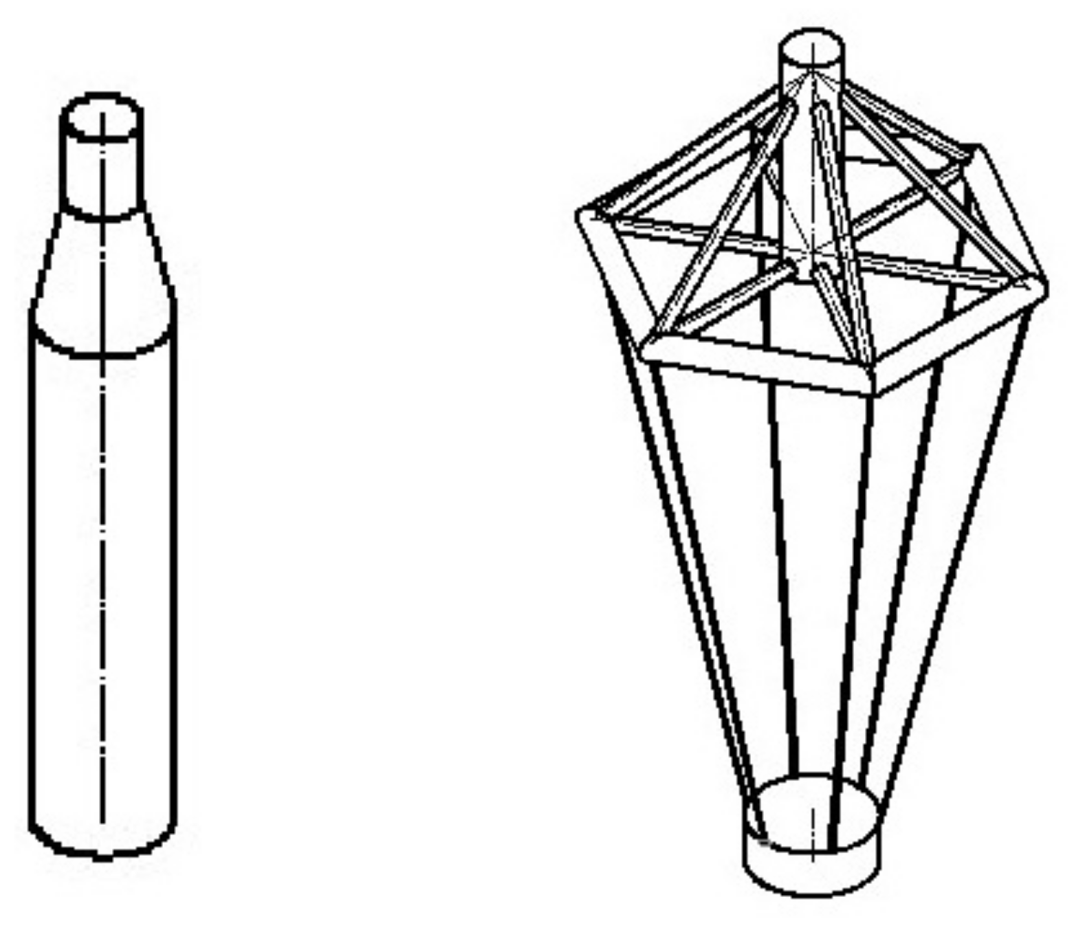
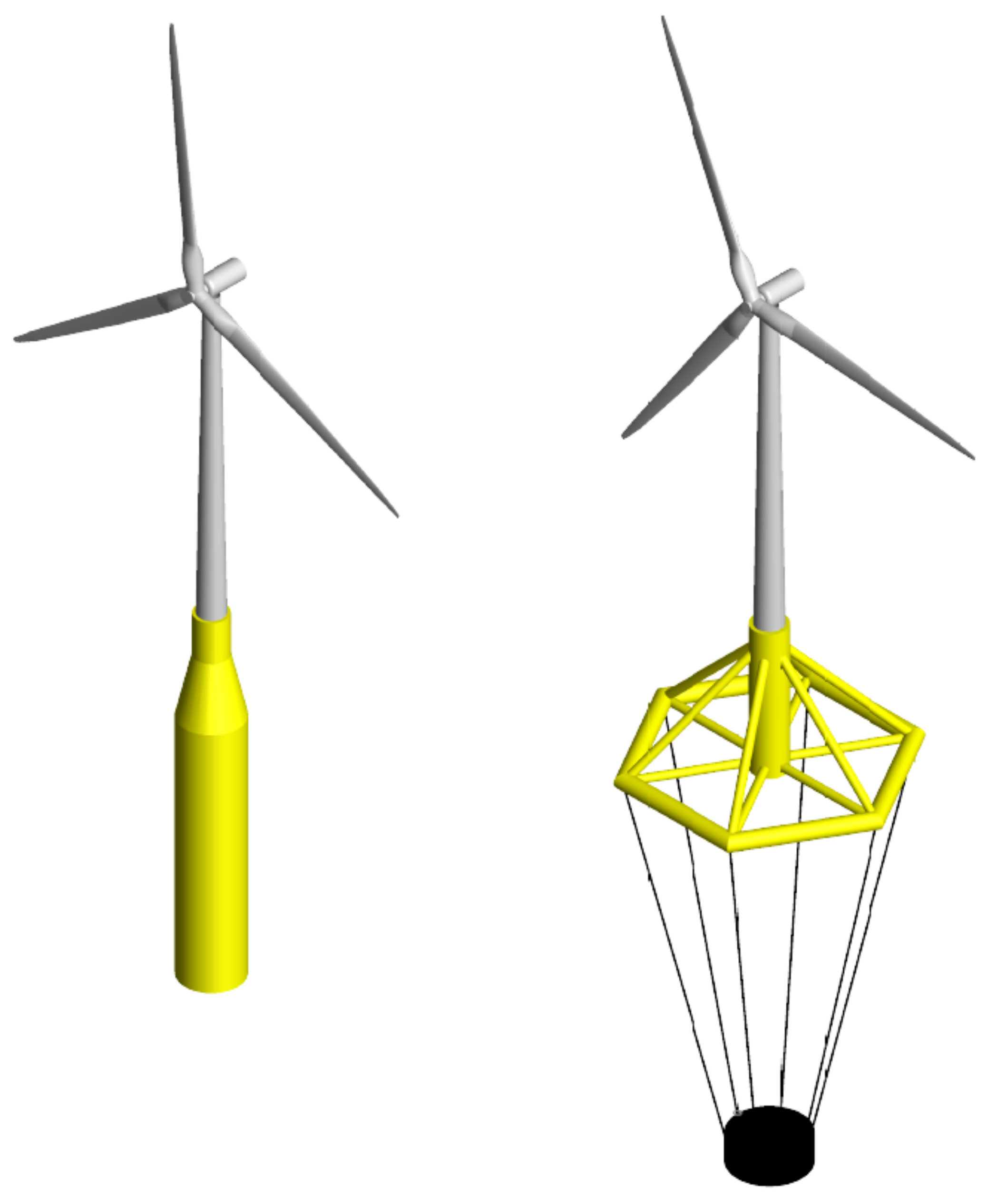
3.3. Choice of the Best Floating Platform

The search for the best floating platform started from the list of all the substructures that the market offers, from which the field was narrowed down to the two concepts that guaranteed good stability at low cost: the spar-buoy and Saipem’s hexafloat [64] (Figure 15 represents the standalone platforms, while Figure 16 represents the platforms with the respective wind turbines).

Using the in-house model, the performances of the two models were compared, in order to choose the most suitable concept for our case study. The geometry of the two concepts has been optimized through a genetic algorithm in order to obtain maximum stability at minimum cost [25]. The key data about the floaters is summarized in

Table 5. Floaters properties.

Spar-Buoy		Saipem’s Hexafloat
Platform diameter	14.75 m	Central column diameter	8.38 m
Platform height	88 m	Central column height	35.25 m
Concrete height	15.64 m	Side length	30 m
Sea water height	17.85 m	Ballast $z_{CoG}$	−99.45
		Ballast diameter	10 m
Mass (steel)	23,230 t	Ballast mass	3304 t
Density (S355 steel)	8500 kg/m3	Density magnetite	5200 kg/m3

. The software package ANSYS Aqwa [28] aims to obtain a parametric description of the floating body in the frequency domain for a discrete range of wave frequencies adopting the panel method. These coefficients are required in order to assemble a time-domain hydrodynamic model.

The in-house model was used by inserting the characteristics of the two platforms, in order to extrapolate the capacity factor of the two concepts. To do this, the 63 simulations reported in Figure 13 were carried out, observing few differences in average power produced between tests with the same mean-wind speed $V_0$ and different wave conditions (less than 0.01%). Starting from this assumption, further tests were carried out for the $V_0$ values that were not included in the 63 triads, in order to obtain an average power value for each $V_0$. The weighted sum of each power was then carried out in relation to the probability of having the corresponding mean-wind speed $V_0$, obtaining the global average power of the system. By dividing the value obtained by the nominal power (5 MW), the capacity factor of the two substructures was obtained (

Table 6. Capacity factors of the two different platform concepts.

	Spar-Buoy	Saipem’s Hexafloat
Capacity factor	45.2%	45.5%

).

Note that the capacity factor values thus obtained are approximately 3% lower than that indicated in Table 4 when the wind resource was analyzed: this is motivated by the fact that an offshore floating wind turbine moves in the sea, thus not remaining fixed in the position of maximum exploitation of the source (as it happens with an onshore wind turbines or with bottom fixed offshore wind turbines).

Observing the energy needs of Pantelleria, it was planned to design a wind farm including 5 turbines of 5 MW.

Considering a commercial stage (CS) of 85.54 €/kW [65], for $n_{turb}$= 5 turbines and $tur{b}_{size}$ = 5 MW:

$$OPEX=CS\ast n_{turb}\ast tur{b}_{size}$$

(99)

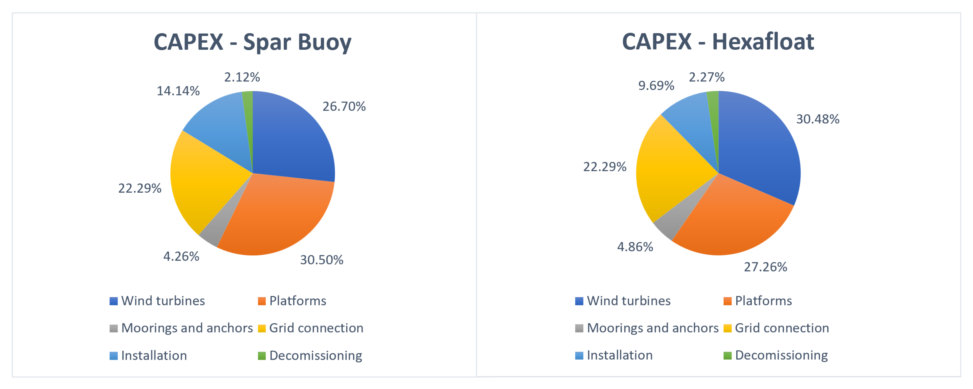
The largest share of CAPEX is split between turbine, platform, grid connection and installation cost [66,67], as can be seen in Figure 17.

The yardstick of choice for the best substructure is the LCOE (levelized cost of energy in €/kWh), whose formulation is as follows:

$$LCOE=\frac{I_0+{\sum }_{t=1}^n\frac{A_t}{{(1+i)}^t}}{{\sum }_{t=1}^n\frac{M_{el}}{{(1+i)}^t}}$$

(100)

where:

• $I_0$: Capital expenditure (CAPEX) in €
• $A_t$: Annual operating costs (OPEX) in year t
• $M_{el}$: Produced electricity in the corresponding year in kWh
• i: Weighted average cost of capital (WACC) in %
• n: Operational lifetime in years
• t: Individual year of lifetime (1, 2, .., n)

Table 7. LCOE internal parameters for the two platform concepts.

LCOE Parameter	Spar-Buoy	Saipem’s Hexafloat
CAPEX	121.74 M€	106.63 M€
OPEX	2.14 M€	2.14 M€
WACC (i rate)	8%	8%
Useful life	25 years	25 years
Capacity factor	45.22%	45.53%
Productivity net	98.99 GWh	99.64 GWh
LCOE	136.82 €/MWh	121.70 €/MWh

shows the comparison between the various items that make up the LCOE. The choice of the optimized hexafloat platform is more convenient, both from a performance point of view (slightly higher capacity factor), and from the economic point of view (LCOE).

3.4. Offshore vs. Onshore Investment

Once the substructure with the lowest LCOE was chosen, this was compared with the onshore case study with the highest productivity in Italy (Savignano Irpino, AV), to verify the convenience of the offshore investment.

Also in this case a wind farm with 5 turbines of 5 MW was considered. Considering a commercial stage (CS) of 36.86 €/kW [65], the OPEX was estimated using Equation (99).

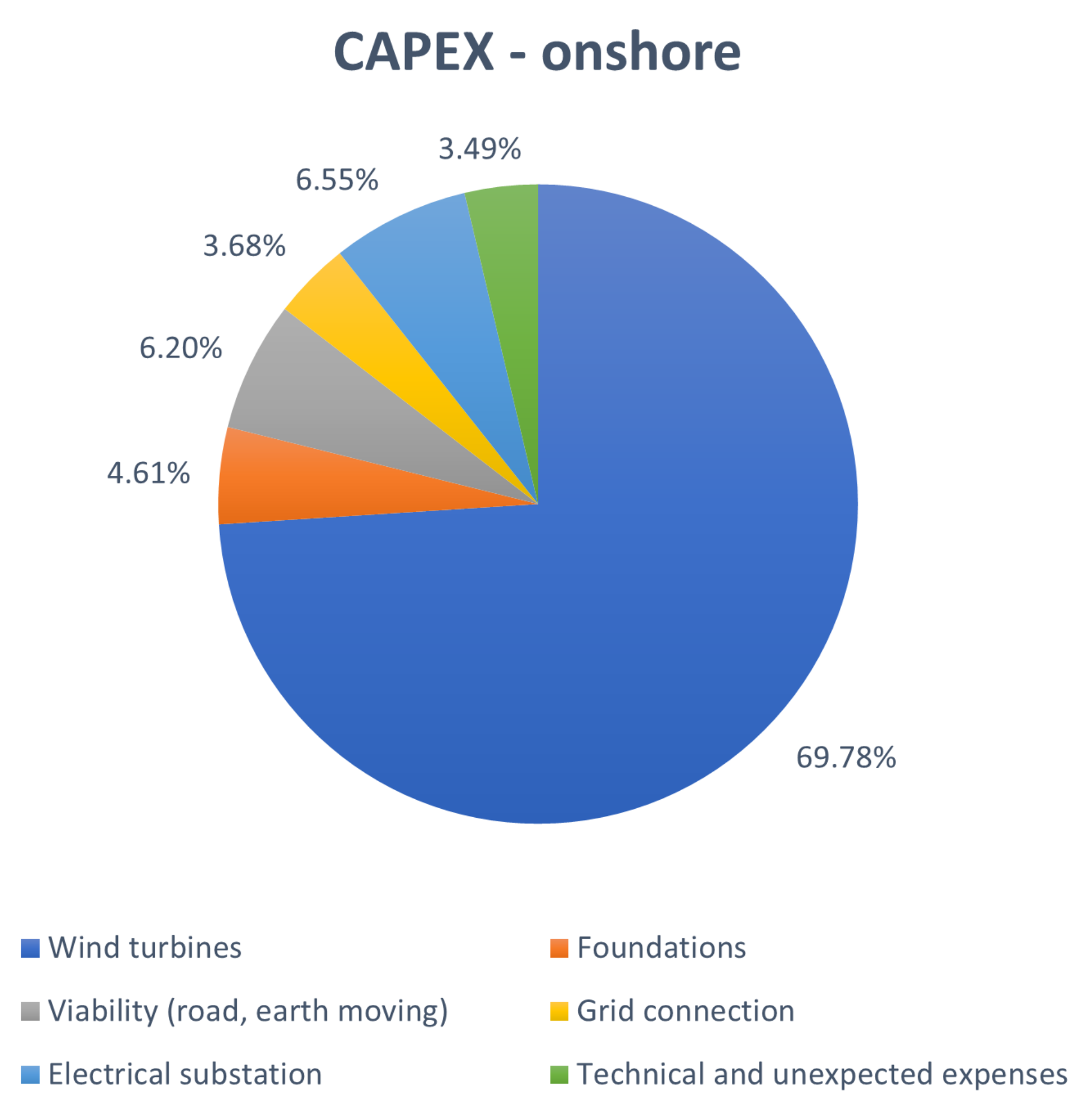
As can be seen in Figure 18, the offshore CAPEX is mainly composed of the cost of the wind turbines (almost 70%), while it was only 27% in the offshore case, which therefore has other relevant cost items besides the turbines. Specifically, in addition to the wind turbine, the offshore floating wind farm is characterised by highly impacting costs of platforms, installation operation and connection to the electrical grid.

In

Table 8. LCOE internal parameters for an onshore turbine.

LCOE Parameter	Value
CAPEX	28.61 M€
OPEX	0.92 M€
WACC (i rate)	8%
Useful life	25 years
Capacity factor	38.74%
Productivity net	84,832 MWh
LCOE	42.45 €/MWh

the values of the internal parameters of the LCOE are shown. Nowadays an onshore investment is approximately three times cheaper than an offshore investment.

Assuming an average CF = 30% for large size onshore wind farms, the calculated LCOE amounts to 65.31 €/MWh.

4. Conclusions

This work had as main objective the creation of a comprehensive model capable of accurately reproducing the behavior of an offshore floating wind turbine, in order to study a suitable application in the Mediterranean Sea. The choice to build an in-house model instead of making use of the FAST model, which is the reference software for offshore wind turbines modeling, was related to a need for higher flexibility and accessibility. The model was developed on Simulink-MATLAB, enabling a convenient learning curve of the tool and permitting the final user to observe the evolution of all intermediate variables. In addition, since the ultimate goal of this work was to optimize the geometrical dimensions of two platforms and verify their performances, the new model was developed with a particular view at the versatility in dealing with different floating platforms. The reliability of the in-house model was measured by comparison with FAST: obtained results were faithful, with an average RMSE on position and output power lower than 2%.

Once the hydrodynamic data were extracted from the Aqwa software for the two optimized substructures (i.e., Spar and Hexafloat), these were inserted into the model. By carrying out various tests consistent with the meteoceanic surveys at the identified site off Pantelleria island, the capacity factors for the two concepts were obtained; for this purpose, a 5 MW reference wind turbine was used. By carrying out a comparison of the LCOE values, the Hexafloat structure was identified as the most convenient in terms of performance and cost-effectiveness.

A final comparison was made between the LCOE obtained for the optimized offshore installation and the LCOE corresponding to an onshore plant in Italy, noting that there is still a huge difference between the profitability of the two investments: offshore wind farms LCOE is almost the double of the onshore ones. However, in Italy as in the rest of Europe, there is a huge need for enabling the implementation of new wind farms, ensuring high levels of productivity and limiting the environmental, social and landscape impact of installations. In addition to the revamping and repowering of existing wind farms, more and more investments in offshore technologies are making their way. While bottom-fixed turbines have a limited remaining potential because of the need of shallow depths, the exploitation of floating offshore wind turbines will be fundamental for the provision of an environmentally, socially and economically sustainable energy mix. The main objectives to be achieved in floating offshore wind industry for enabling a large uptake of the technology are the reduction of platform CAPEX (Figure 17), that can be reached through an accurate and site-specific optimization of hulls; the exploitation of novel installation methods; and the use of innovative electrical system for power transmission to mainland. All this is expected to decrease the overall LCOE of new installations, that will be able to reduce environmental & landscape impact.

Despite the proposed model has demonstrated high reliability and accessibility, it has some clear limitations:

• Computational burden: based on the performed comparison, the in-house model requires about twice the computational time to carry out a simulation compared to FAST. However, it is noticeable that this time is still less than the simulation time, thus not limiting the possibility of carrying out real-time simulations.
• The platform, tower, nacelle and blades are currently modeled as rigid bodies.
• Concerning aerodynamics, the implementation of the BEM theory is currently characterized by a tolerance value higher than that of FAST, in order to enhance the resolution algorithm convergence and shorten the calculation time.
• The used mooring theory, MAP++, is quasi-static, while mooring dynamics can also be affected by considerable inertial loads.
• The model is very limited in the representation of the overall power output, as the electrical conversion is currently simply represented by a generator efficiency value.

Starting from current model limitations, future works will have to focus on the following aspects, with the aim of further enhancing model reliability and enabling wider applications:

• The elastic theory could be applied to the modeling of platform, tower, nacelle and blades, in order to further increase the model accuracy.
• The MAP++ quasi-static theory could be replaced with a dynamic theory, leading to higher fidelity in representing mooring effects on the floating platform.
• The integration of accurate electrical machines and converters models could provide important information for the study of arrays, power connections and, more in general, on the impact of large floating wind farms in power networks.
• The insertion of the in-house model in a genetic algorithm in order to obtain new and innovative substructure concepts.