Article

Estimating Energy Forecasting Uncertainty for Reliable AI Autonomous Smart Grid Design

1
Department of Computer Science, Trent University, Peterborough, ON K9L 0G2, Canada
2
Department of Mathematics, Trent University, Peterborough, ON K9L 0G2, Canada
3
National Institute of Standard, Giza 12212, Egypt
4
School of Computing, Queen’s University, Kingston, ON K9L 3N6, Canada
5
Lowfoot Inc., Toronto, ON M5A 2B7, Canada
*
Author to whom correspondence should be addressed.
Energies 2021, 14(1), 247; https://doi.org/10.3390/en14010247
Submission received: 24 November 2020 / Revised: 24 December 2020 / Accepted: 1 January 2021 / Published: 5 January 2021
(This article belongs to the Special Issue Artificial Intelligence Technologies for Electric Power Systems)

Abstract

:
Building safe, reliable, fully automated energy smart grid systems requires a trustworthy electric load forecasting system. Recent work has shown the efficacy of Long Short-Term Memory neural networks in energy load forecasting. However, such predictions do not come with an estimate of uncertainty, which can be dangerous when critical decisions are being made autonomously in energy production and distribution. In this paper, we present methods for evaluating the uncertainty in short-term electrical load predictions for both deep learning and gradient tree boosting. We train Bayesian deep learning and gradient boosting models with real electric load data and show that an uncertainty estimate may be obtained alongside the prediction itself with minimal loss of accuracy. We find that the uncertainty estimates obtained are robust to changes in the input features. This result is an important step in building reliable autonomous smart grids.

1. Introduction

Confident predictions are necessary to build reliable, fully Artificial Intelligence (AI) automated smart energy grid systems [1,2,3,4,5,6]. Load predictions produced without any information about their uncertainty are unsafe [7] when critical autonomous decisions are being made in energy production and distribution. Current forecasting models normally do not provide information about uncertainty in their predictions, which can lead to costly and risky decisions and affect current efforts to produce a reliable smart energy grid system [8]. This is a problem for many AI applications, such as autonomous vehicles, where the lack of consideration for uncertainty can be dangerous [9]. Therefore, for safe, reliable, autonomous artificial intelligence systems and for safe prediction-based decisions, evaluating the degree of uncertainty is paramount [10].
At the same time, the efficient allocation of resources is a primary goal of the electric power industry, which includes the production, transportation, and distribution of energy. An accurate forecast of the future electric load is integral to achieving this, as it allows utility companies to make informed decisions for planning and operations [2,3,11]. Accurately predicting the hourly load, known as Short-Term Electric Load Forecasting (STELF), allows utilities to make these decisions in real-time and saves millions of dollars normally wasted due to overload or underload costs as well as reducing CO2 emissions [4,12,13,14].
Obtaining confident and accurate estimates for learning models through data-driven methods has been the subject of intensive research [4]. A recent survey [13] showed that previous studies primarily used artificial neural networks (ANNs) and support vector machines (SVMs), with decision trees and various statistical methods making up the remainder. Of these, ANNs have become the most common choice due to advances in deep learning and the development of neural net architectures such as the long short-term memory (LSTM) network [15], designed for sequence modeling and time series tasks. LSTM networks have been employed successfully for a wide range of applications, including short-term electric load forecasting [13,16,17,18,19]. At the same time, tree-based algorithms such as gradient-boosted trees have become widely used in industry and machine learning competitions due to lower computation requirements, ease of interpretation and tuning, and better performance on smaller datasets, and have recently been applied to load forecasting as well [20,21,22].
In this paper, we present the implementation and testing of two methods for estimating uncertainty of short-term electrical load prediction, based on two popular machine learning algorithms: LSTM and gradient boosting regression (GBR). The contributions are fourfold. First, we developed two energy forecasting computational models using deep learning techniques. LSTM represents a class of advanced artificial recurrent neural networks (RNN) that has been shown to be efficient in many applications. However, to our knowledge, this is the first time that LSTM has been applied together with Monte Carlo dropout regularization to quantify the prediction uncertainty for energy forecasting. Second, we applied the optimization algorithm GBR to energy forecasting. More importantly, using the properties of the GBR to accept an arbitrary differentiable loss function, we were able to construct prediction intervals to measure the uncertainty of the prediction. Third, the applicability and effectiveness of the models are verified and analyzed using real-world data–a benchmark dataset on electricity load forecasting. The impact of implementing such methods on predictive accuracy, as well as the effect of input features on the produced uncertainty are also examined. Lastly, experimental results show that the models achieved high prediction accuracies in terms of the Mean Absolute Percent Error (MAPE) and that uncertainty estimates can be obtained with minimal cost to accuracy.
The rest of the paper is organized as follows. In Section 2, we introduce the algorithms, uncertainty estimation, and the design of the learning models. Section 3 describes the processing of the dataset, implementation, and experimental results. Finally, some conclusions and future work are presented in Section 4.

2. Algorithms of Learning Models

We first discuss the two algorithms for STELF and then present techniques for producing a prediction interval for each.

2.1. Long Short-Term Memory

Long short-term memory (LSTM) is a recurrent neural network architecture that has gained widespread popularity due to its ability to model long-term dependencies and automatically extract features [15,16,23,24]. It has also been shown that the ANN vanishing gradient problem, which affects ordinary RNNs, does not occur for the LSTM cell [15,16,23,24]. This has made it a favoured choice for time series modeling [18,19], including recently, electric load forecasting [5,17]. There are several variants in use today, but in this paper, we use the standard architecture presented by Graves and Schmidhuber [23].
The key idea behind LSTM is to introduce a memory cell to standard RNN architecture (Figure 1). This memory cell, built out of simple nodes in a specific pattern, allows the LSTM module to retain information across many timesteps when needed [25]. The flow of information to and from the memory cell is controlled by three “gates”, each of which performs a multiplication on the information passing through to determine how much to allow past.
We will describe the network using a similar presentation to those by Kong [26] and Lipton [25]. We denote the input to the LSTM module at timestep t with x t and its output with y t , in our case, both in MWh units. We represent the state of the memory cell with h t . Each gate itself is a neuron with a sigmoid activation function σ , and uses the input x t and previous memory cell state h t 1 to produce a set of values between 0 and 1 representing the amount of information let through. The W matrices are weight matrices for each neuron.
We first create a candidate state g t to potentially update the memory cell with, using a tanh activation function:
g t = tanh ( W g x x t + W g h h t 1 + b g ) ,
where W g x represents the weights between the input x and the state g, W g h represents the weights between the previous state h and the state g, and b g represents the bias.
The first of the gates, the forget gate f t , will determine how much of the memory cell state we preserve between timesteps and is given by:
f t = σ ( W f x x t + W f h h t 1 + b f ) ,
where W f x and W f h represent the weights between the gate neuron f and the input x and previous state h, respectively. As above, b f represents the bias. The input gate i t will determine how much of the candidate state g t will be added to the memory cell, and is given by
i t = σ ( W i x x t + W i h h t 1 + b i ) ,
where W i x and W i h represent similar weight matrices as above for the input x and the previous state h, and b f represents the bias. The memory cell is then updated with the new values,
h t = i t g t + f t h t 1 ,
where ⊙ denotes an elementwise or Hadamard product. The output gate is calculated in a similar manner to the other gates:
o t = σ ( W o x x t + W o h h t 1 + b o ) ,
where W o x and W o h represent similar weight matrices as above for the input x and the previous state h, and b o represents the bias. To produce the output y t , the contents of the memory cell are passed through the gate and a tanh function to constrain the values to the same range as an ordinary tanh hidden unit [25].
y t = o t tanh ( h t ) .

2.2. Uncertainty Estimation for LSTM

Our goal is to measure the uncertainty of the LSTM-based prediction. There may be multiple sources of uncertainty present as well as inherent noise, but in this work we will restrict discussion to the model-specific sources of uncertainty, resulting from uncertainty in our model parameters—the connection weights. This is usually known as model or epistemic uncertainty and will be reduced as more data is collected [10,19,27].
To measure this type of uncertainty, we introduce a prior probability distribution for each weight in the neural network, usually Gaussian, and attempt to find a posterior distribution rather than a single estimate. This type of network is known as a Bayesian neural network (BNN), but due to the large number of parameters involved, it is difficult to solve traditionally [10,19,28,29]. However, it has been shown that dropout regularization—the technique of stochastically dropping out neurons to reduce overfitting—can also be used to approximate the results of a BNN without the difficulty found in the conventional approach [10,19,28]. In this regularization technique, a small fraction of units throughout the network are muted with every training stage [30,31]. This reduces codependencies between neurons that lead to overfitting and force the model to learn more robust features.
Normally, in the prediction stage, no neurons are dropped and the entire network is used. However, by continuing to drop out neurons during the prediction stage and sampling multiple times—an algorithm called Monte Carlo dropout or MC dropout—we exchange some of the predictive power of the full network in order to create a distribution of predictions. As shown in [28], this can be thought of as sampling from the posterior distribution of a Bayesian network; as a result, we can estimate the variance of the posterior and, therefore, the model uncertainty by means of the variance in these predictions [10,19,28,32].
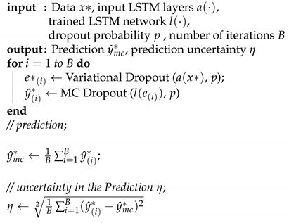
Our algorithm for estimating model uncertainty using Monte Carlo dropout follows the steps outlined in [10]. A neural network can be represented by a function f W ( · ) , where f captures the network structure, and W is the set of neural network weights. After training our neural network and feeding it with new data x * , our goal is to evaluate the uncertainty of our neural network prediction y ^ * = f W ( x * ) by calculating the prediction standard error η , which allows us to create an α -level prediction interval with
[ y ^ * z α / 2 η , y ^ * + α / 2 η ] ,
using the z score z α / 2 . The detailed algorithm for MC dropout is as follows: Given a new input data x * to a trained neural network, we compute the neural network output prediction while randomly dropping out each hidden unit with certain probability p. The feed forward stage is repeated with stochastic dropout B times, resulting in the predicted values { y ^ 1 * , , y ^ B * } .
The sample variance is then Var [ f W ( x * ) ] , and the model uncertainty can be approximated as [10]
Var [ f W ( x * ) ] = 1 B i = 1 B ( y ^ ( i ) * y ^ m c * ) 2 ,
where
y ^ m c * = 1 B i = 1 B y ^ ( i ) * .
The desired prediction standard error η can now be calculated using
η = 1 B i = 1 B ( y ^ ( i ) * y ^ m c * ) 2 2 .

2.3. Gradient Tree Boosting

For comparison, we also evaluate the performance of a second popular algorithm, gradient boosting regression (GBR). Boosting is a meta-algorithmic technique whereby a model is built from an ensemble of individually weak models, step by step. At each stage, the new model being added attempts to improve on the performance of the current ensemble. Implementations of gradient boosting such as XGboost have proved extremely effective in real-world scenarios and machine learning competitions, offering both speed and accuracy.
We provide an overview of the technique, as described in [22]. Given a dataset with n training examples consisting of an input x i and expected output y i , a tree ensemble model ϕ ( x i ) is defined as the sum of K regression trees f 1 , f 2 , . . . , f K :
y i ^ = ϕ ( x i ) = k = 1 K f k ( x i ) .
To evaluate the performance of a given model, we choose a loss function l ( y i ^ , y i ) to measure the error between the predicted value and the target value, and optionally add a regularization function Ω ( f k ) which operates on trees and calculates a penalty. The loss L ( ϕ ) of the ensemble is then
L ( ϕ ) = i n l ( y i ^ , y i ) + k K ( Ω ( f k ) ) .
The regularization function, if used, is designed to penalize more complex trees and acts as an ”Occam’s razor“ term that encourages simpler models. Our goal is to minimize L ( ϕ ) and, to do so, we introduce each f k iteratively. Assume that the ensemble currently contains K trees. We add a new tree f K + 1 that minimizes
i n l ( y i ^ , y i + f K + 1 ( x i ) ) + Ω ( f k ) ,
or in other words, we greedily add the tree that most improves the current model as determined by L. We train the new tree using this objective function; this is often done by approximating the objective function using the first- and second-order gradients of the loss function l ( y i ^ , y i ) using the method given by Friedman et al. [33].

2.4. Uncertainty Estimation for GBR

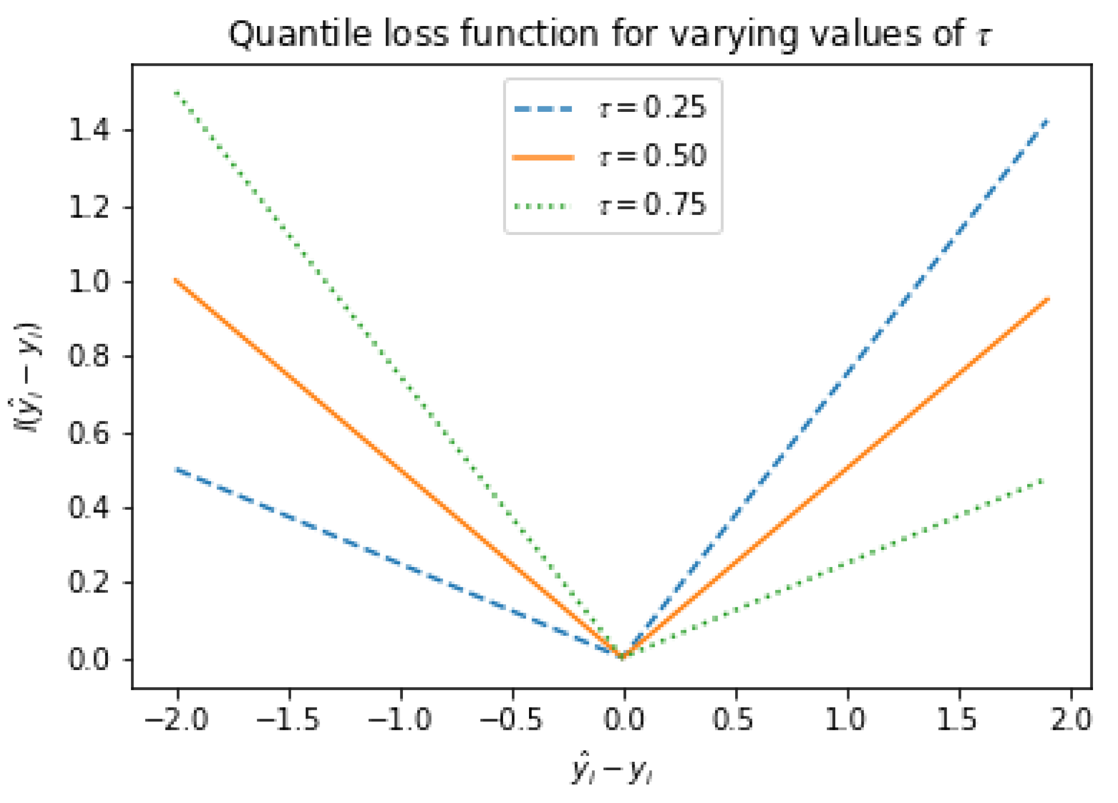
As the first few trees added will dominate the model performance, we cannot randomly drop out trees during prediction in order to construct a prediction interval. Instead, we adapt a technique described in [34] whereby the loss function is altered, training the model to predict values other than the mean. By predicting an upper bound and lower bound at a certain level of confidence, we can train the model to output the uncertainty in its own prediction. The loss function we choose is known as the quantile or pinball loss function, a generalization of the Mean Absolute Error (MAE) used for the LSTM model, and for a given prediction y i ^ , target value y i , and desired quantile τ , is defined as
l τ ( y i ^ , y i ) = y i ^ > = y i τ | y i ^ y i | + y i ^ < y i ( 1 τ ) | y i ^ y i | .
As shown in Figure 2, this produces a tilted version of the MAE loss function determined by the parameter τ , with τ = 0.5 reducing to standard mean absolute error. Minimizing this loss will train the model to produce a prediction of the τ -th quantile [35], and training two additional models—one to predict an upper quantile, and one to predict a lower quantile—allows us to construct a prediction interval for the gradient-boosted prediction. For our experiments, we select τ = 0.95 and τ = 0.05 to produce a 90% prediction interval.

3. Experiment and Results

We now discuss our implementations of the methods described above, as well as empirical results.

3.1. Model Implementation

We use the Python-based scikit-learn package [36] and the TensorFlow and Keras libraries [16,24,37,38] to implement three learning models. The first model is the standard LSTM architecture as used in practice [17,26], consisting of the input layer, three LSTM hidden layers with 50 neurons each, and a single neuron in the output layer.
The second model implements uncertainty estimation as described above, by performing Monte Carlo sampling with dropout to approximate a Bayesian posterior distribution for the predictions (Algorithm 1). We then construct a 90% interval based on the sample variance as the uncertainty estimate. The Mean Absolute Error (MAE) loss function and the Adam version of stochastic gradient descent were used with Keras and Tensorflow to optimize the LSTM models.
The third model is a gradient boosting regressor implemented using the GradientBoos tingRegressor function from the sci-kit-learn package [36] and optimized for Mean Absolute Error (MAE) in MWh unit. Two auxiliary models are implemented the same way, but optimized using quantile loss for the 95th and 5th quantiles. The 90% prediction interval is constructed using the outputs from the auxiliary models, while the main model provides the prediction. Table 1 lists the configuration parameters for the implementation.
Algorithm 1: MC dropout Algorithm for model uncertainty.
Energies 14 00247 i001

3.2. Data and Feature Selection

The data used in this paper was obtained from the European Network on Intelligent Technologies (EUNITE) 2001 competition on electricity load forecasting [39]. The data was collected by the Eastern Slovakian Electricity Corporation for two years from 1 January 1997 until 31 December 1998, and contains the following features:  
- Half-hourly electricity load in MWh.
- Daily average temperature in Celsius.
- Annual holidays.  
The objective of the original competition was to predict the daily peak electricity load for the 31 days of January 1999 using the given historical data. For this paper, our objective is to instead predict the electricity load for each half-hour for the same time period and compare the forecast with actual consumption.
The EUNITE competition data has been studied by many authors [40,41] to investigate the relationship between load data and other features such as temperature, weekdays, and annual holidays.

3.2.1. Temperature Effects

References [40,41] show from the load and average daily temperature data that the electricity load has high consumption in the winter (September–March) due to heater usage in the winter, and low consumption in the summer (April–August). This behavior indicate a strong relationship between the electricity load and the weather conditions represented by temperature. A negative correlation with coefficient −0.8676 was found between the daily peak load and daily average temperature over the two years [40,41], showing this strong relation.

3.2.2. Weekday Effects

Examination of load data during the weekdays shows that a periodic weekly pattern exists in the consumption. References [40,41] show that on most Saturdays and Sundays (the weekends), the load is lower than on weekdays (Monday–Friday). In addition, electricity peak load usually occurs on a Wednesday.

3.2.3. Holiday Effects

The analysis for the two-year historical load data shows that the load usually reduces on holidays [40,41]. The load demand also depends on the type of holiday; for example, on Christmas or New Year, the electricity consumption is affected more compared to other public holidays.

3.2.4. Feature Selection

For high-accuracy load forecasting, our model needs the most descriptive input features that have the highest correlation with the output forecasting variable and the highest degree of linear independence.
From the above data analysis, the best candidate input features are the past half-hourly loads, the average daily temperatures, and the type of day [40,41].

3.2.5. Half-Hourly Load

Past half-hourly load is a very good indicator of the next timestep’s load. Including the past half-hourly loads as a key feature is very important for high-accuracy forecasting.

3.2.6. Average Daily Temperature

From the above data analysis, electricity load and the average daily temperature have a high negative correlation. Therefore, the average daily temperature is a crucial feature for our forecasting model.

3.2.7. Weekday Indicator

The weekday effect on electricity load was shown in the data analysis as a pattern in references [40,41]. Therefore, the type of day can be encoded numerically as a feature in our forecasting model to enhance its performance. This can be done in Python by using the method, date.weekday(), which returns the day of the week as an integer, where Monday is 0 and Sunday is 6.

3.2.8. Public Holidays

Public holidays have a significant effect on users’ behaviors for electricity consumption. Hence, inclusion of a binary indicator 0/1 for public holidays in our forecasting model will benefit its accuracy.

3.2.9. Time Series Modeling

After encoding indicators of both weekdays and public holidays as numerical values, the EUNITE competition data was framed as multivariate time series data consisting of sequences of records ordered by date and time, as shown in Table 2.

3.2.10. Data Normalization

The range of values for the EUNITE competition data varies widely with feature, which affects both the accuracy and the stability of our forecasting model [16,24,37,38]. Therefore, the ranges of all features have been normalized by rescaling each feature to lie within [ 0 , 1 ] . This scaling was done in Python using the MinMaxScalers method from the sklearn package [24,37].

3.2.11. Convert Data to Input–Output Pairs

The main task for our models in a supervised machine learning setting is to learn the function that maps inputs to an output, based on examples from labeled training data consisting of known input–output pairs [16,24].
The EUNITE competition data must be reframed as a supervised machine learning problem in order to be handled by our models for forecasting electricity load.
Therefore, the multivariate time series was converted to input–output pairs using a sliding window method, in which prior time steps are used as features for predicting the next time step [38,42,43].

3.3. Splitting Data into Train and Test Sets

The two years of historical data was split into training and testing sets, with 80 % for training and 20 % for testing. The training and testing sets were split into input and output variables, and finally, the inputs were reshaped into the 3D format expected by our models, namely, [samples, time steps, features] [16,24,37,38]. The training set was used first to train our models, then the testing set was used to evaluate it.

3.4. Experimental Results

The three models—namely, the standard LSTM Model, the Bayesian LSTM model, and the GBR model—were trained and used to forecast the electricity load for the month of January 1999. The accuracy of the load forecast is measured by way of two error metrics: the Root Mean Square Error (RMSE) in MWh units and the Mean Absolute Percent Error (MAPE). The RMSE is the standard deviation of the prediction errors and is defined as follows [40,41]:
RMSE = 1 N i = 1 N y i y ^ i 2 ,
where y i is the target value, y ^ i is the predicted value, and N is the total number of values. The MAPE is calculated by taking the average of the unsigned percentage errors as follows [40,41]:
MAPE = 1 N i = 1 N y i y ^ i y i × 100 .
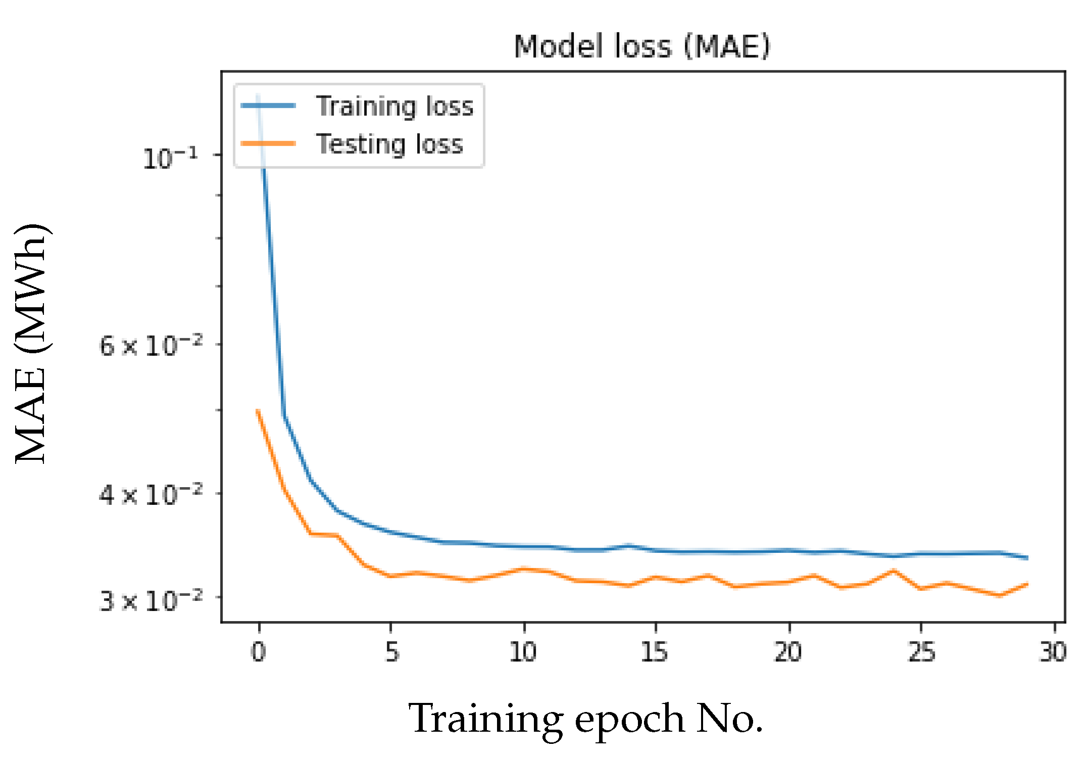
The behavior of these metrics during the training sessions for each model is shown in Figure 3 and Figure 4. We note that the loss drops with each epoch and stabilizes over time, indicating that the models are sufficiently trained without overfitting.
Results from the standard LSTM model are shown in Figure 5. We can see that the model is efficient in comparing the prediction mean and the actual values. In fact, the error percentage measured as MAPE is less than 3%, as shown in Table 3.
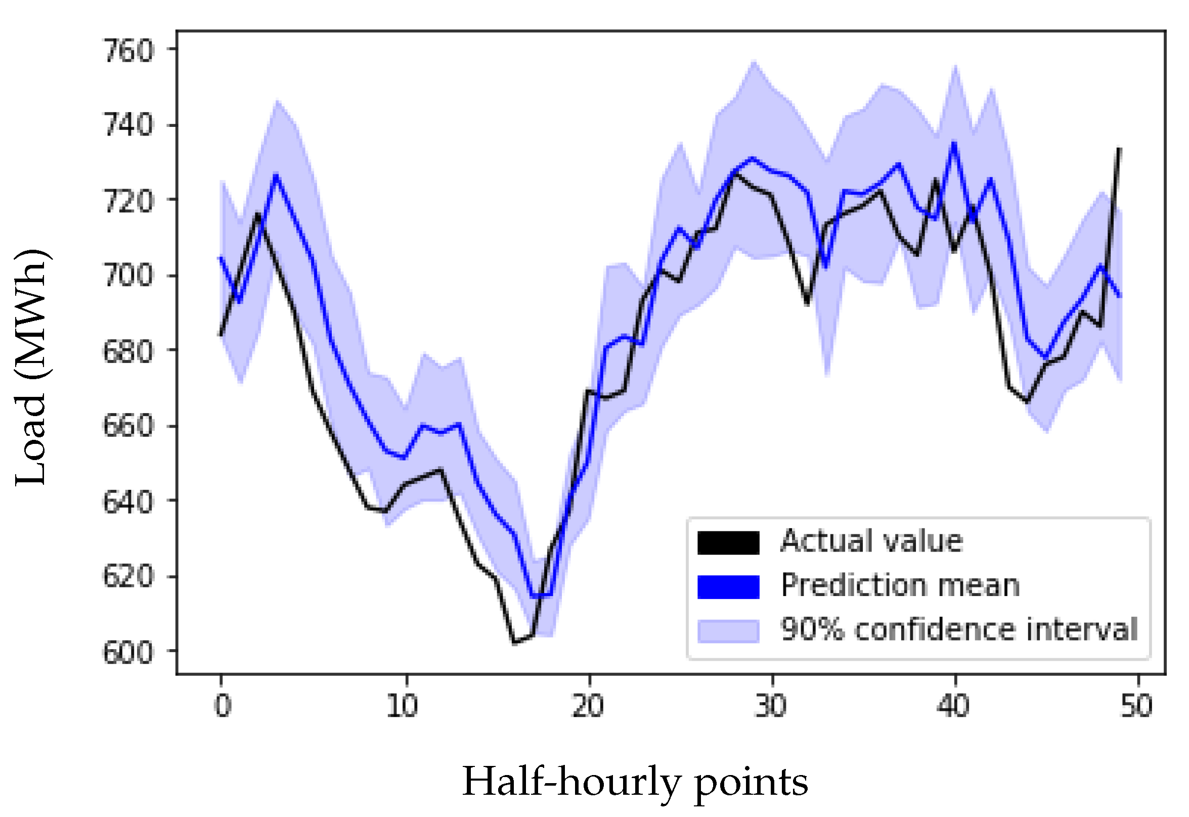
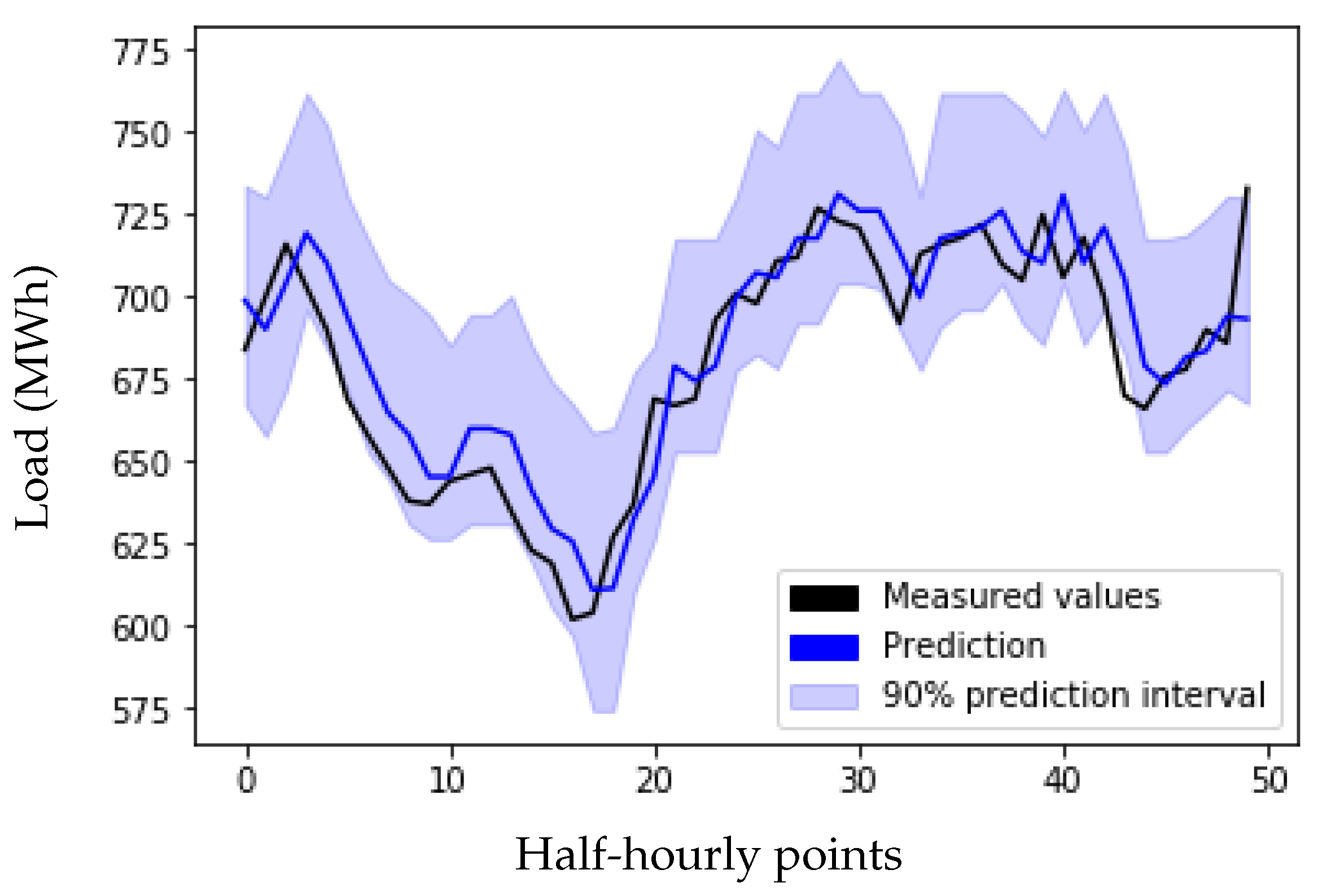
The January forecast obtained from the Bayesian LSTM model is shown for 50 timesteps in Figure 6. We note that the uncertainty band is narrow due to this only being a measure of the model uncertainty and not including other sources of error such as noise. Figure 7 shows the same prediction using quantile regression with the GBR model. As this method does not differentiate between sources of uncertainty but instead captures all types, we note that the prediction intervals are wider than those for the LSTM model.
Table 3 shows the RMSE and MAPE values for each model for the January 1999 testing set. The simple LSTM model shows high accuracy with a MAPE value of 2.3 percent. Introducing MC dropout to the neural network reduces the accuracy of the LSTM model by a small amount. GBR achieves similar accuracy or slightly better accuracy compared to the LSTM model, and as producing a prediction interval does not require any modifications to the main predictive model itself, there is no loss in performance. Overall, the performance of all three models is fairly similar, showing that uncertainty estimates can be obtained with minimal cost to accuracy.

3.5. Uncertainty Analysis

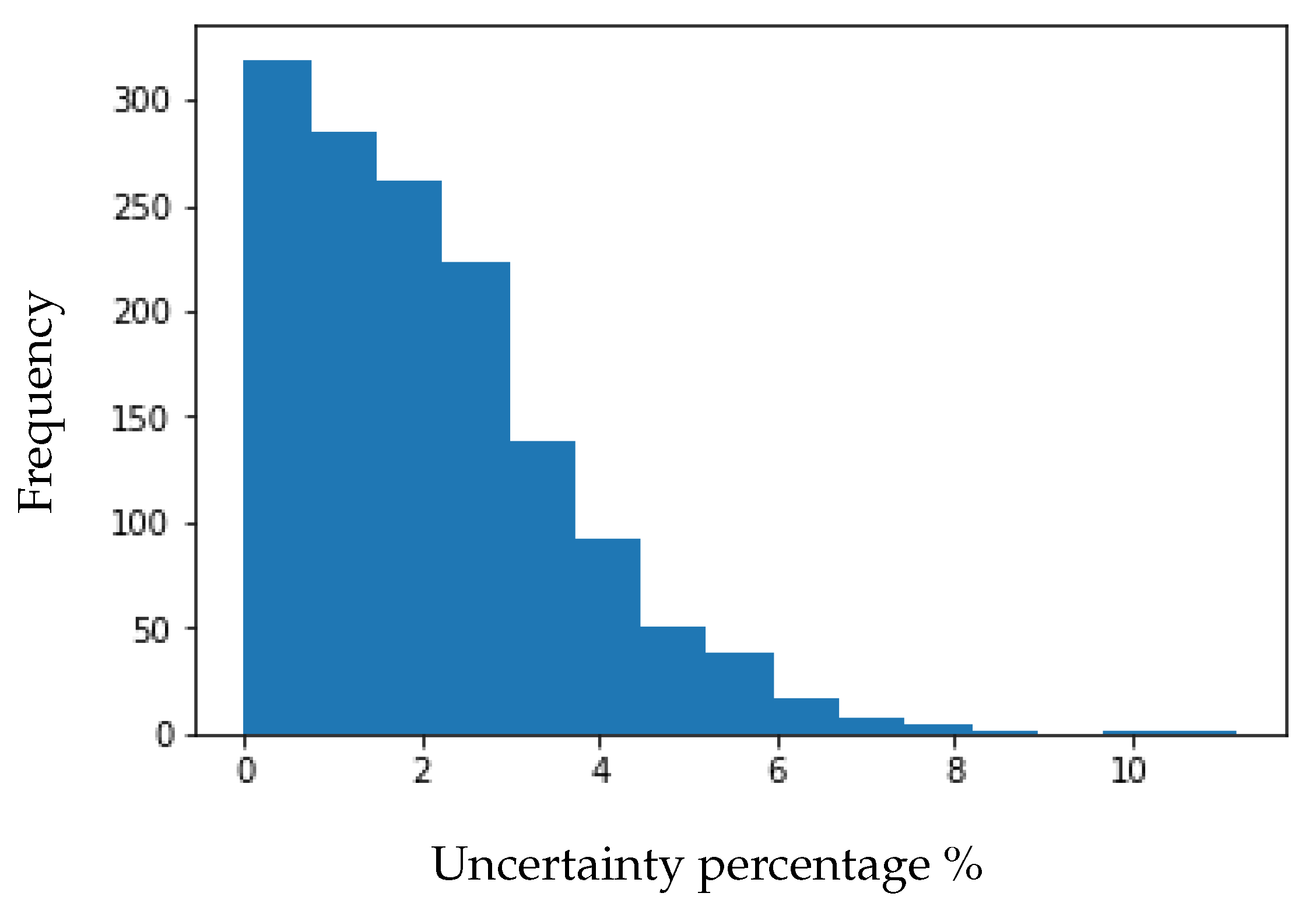
We perform some analysis for the obtained uncertainty values. Figure 8 shows the frequency of the calculated uncertainty as a percentage of the actual load values in the prediction of January 1999 loads. We observe that the frequency decreases for higher percentage values of uncertainty and almost no uncertainty estimates rise above 10%. This behavior reflects the relatively high confidence and low error percentage of our forecasting model.
Table 4 shows the correlation of the percentage uncertainty with the input features used in the prediction of January 1999 load, namely, the past half-hourly loads, the average daily temperatures, type of weekdays, and public holidays. From the figure, the uncertainty has a −0.05 correlation with the past half-hourly loads, a 0.03 correlation with average daily temperatures, and zero correlation with the type of weekdays or public holidays. We see that the model uncertainty is generally independent of the features used as it is a result of the model architecture.

4. Conclusions

With the fast development of machine learning algorithms and their extensive application, estimating model uncertainty has become a significant research area. We implemented and evaluated two methods in quantifying the uncertainty for two popular supervised learning algorithms. This work is one of the few that studies uncertainty for both RNN and tree based algorithms in the area of energy forecasting. An uncertainty measure is critical for applications such as designing reliable AI-enabled autonomous energy smart grids [10]. In addition, uncertainty is also an important metric for energy production and distribution as it allows utility companies to assess the trustworthiness of forecasts before making decisions. Our results demonstrate the effectiveness of the learning techniques, LSTM and GBR, and the uncertainty evaluation methods, using the EUNITE electricity load dataset. Both methods are shown to provide accurate predictions.
There remains much to be investigated in the field of uncertainty estimation and its application to electricity forecasting. Although we only described methods to produce uncertainty estimates for two algorithms used in STELF, these methods can also be extended to other forecasting algorithms. Monte Carlo methods can be used to estimate the degree of uncertainty that can be attributed to the model parameters, by estimating the variance of the posterior. Quantile methods which aim to train separate models to predict upper and lower bounds can provide an overall estimate of the expected distribution. Both techniques provide useful estimates of the risk in real-world scenarios and easy computational implementations for AI-enabled autonomous smart grids.

Author Contributions

Conceptualization, all authors; methodology, M.S. and R.Z.; software, M.S. and R.Z.; validation, all authors; formal analysis, M.S., R.Z., and W.F.; investigation, all authors; resources, W.F. and P.Q.; data curation, M.S. and R.Z.; writing—original draft preparation, M.S., R.Z., and W.F.; writing—review and editing, M.S., R.Z., and W.F.; visualization, M.S., R.Z., and W.F.; supervision, W.F. and P.Q.; project administration, W.F. and P.Q.; funding acquisition, W.F. and P.Q. All authors have read and agreed to the published version of the manuscript.

Funding

This research was funded by the Natural Sciences and Engineering Research Council of Canada (NSERC, Engage grant) and Lowfoot Inc.

Institutional Review Board Statement

Not applicable.

Informed Consent Statement

Not applicable.

Data Availability Statement

Dataset used in this study is open data from EUNITE Electricity Load Forecast 2001 Competition: http://www.eunite.org/knowledge/Competitions.

Acknowledgments

The authors thank the anonymous referees for their significant comments and suggestions that helped to improve the quality of paper.

Conflicts of Interest

The authors declare no conflict of interest.

Abbreviations

The following abbreviations are used in this manuscript:
STELFShort-Term Electric Load Forecasting
AIArtificial Intelligence
LSTMLong Short-Term Memory
ANNsArtificial Neural Networks
SVMsSupport Vector Machines
GBRGradient Tree Boosting
RMSERoot Mean Square Error
MAPEMean Absolute Percent Error
EUNITEEuropean Network on Intelligent Technologies

References

  1. Hong, Y.Y.; Lai, Y.M.; Chang, Y.R.; Lee, Y.D.; Liu, P.W. Optimizing capacities of distributed generation and energy storage in a small autonomous power system considering uncertainty in renewables. Energies 2015, 8, 2473–2492. [Google Scholar] [CrossRef] [Green Version]
  2. Toffanin, D. Generation of Customer Load Profiles Based on Smart-Metering Time Series, Building-Level Data and Aggregated Measurements. Ph.D. Thesis, Università degli Studi di Padova, Padova, Italy, 2016. [Google Scholar]
  3. Saleh, A.I.; Rabie, A.H.; Abo-Al-Ez, K.M. A data mining based load forecasting strategy for smart electrical grids. Adv. Eng. Inform. 2016, 30, 422–448. [Google Scholar] [CrossRef]
  4. Zhou, K.; Fu, C.; Yang, S. Big data driven smart energy management: From big data to big insights. Renew. Sustain. Energy Rev. 2016, 56, 215–225. [Google Scholar] [CrossRef]
  5. Bianchi, F.M.; Maiorino, E.; Kampffmeyer, M.C.; Rizzi, A.; Jenssen, R. An overview and comparative analysis of Recurrent Neural Networks for Short Term Load Forecasting. arXiv 2017, arXiv:1705.04378. [Google Scholar]
  6. Lilliu, F.; Loi, A.; Recupero, D.R.; Sisinni, M.; Vinyals, M. An uncertainty-aware optimization approach for flexible loads of smart grid prosumers: A use case on the Cardiff energy grid. Sustain. Energy Grids Netw. 2019, 20, 100272. [Google Scholar] [CrossRef]
  7. Kabir, H.D.; Khosravi, A.; Hosen, M.A.; Nahavandi, S. Neural network-based uncertainty quantification: A survey of methodologies and applications. IEEE Access 2018, 6, 36218–36234. [Google Scholar] [CrossRef]
  8. Kumari, P.A.; Geethanjali, P. Artificial Neural Network-Based Smart Energy Meter Monitoring and Control Using Global System for Mobile Communication Module. In Soft Computing for Problem Solving; Springer: Berlin/Heidelberg, Germany, 2020; pp. 1–8. [Google Scholar]
  9. McAllister, R.; Gal, Y.; Kendall, A.; Van der Wilk, M.; Shah, A.; Cipolla, R.; Weller, A.V. Concrete problems for autonomous vehicle safety: Advantages of Bayesian deep learning. In Proceedings of the International Joint Conferences on Artificial Intelligence, New York, NY, USA, 9–15 July 2016. [Google Scholar]
  10. Gal, Y. Uncertainty in Deep Learning. Ph.D. Thesis, University of Cambridge, Cambridge, UK, 2017. [Google Scholar]
  11. Kontokosta, C.E.; Tull, C. A data-driven predictive model of city-scale energy use in buildings. Appl. Energy 2017, 197, 303–317. [Google Scholar] [CrossRef] [Green Version]
  12. Grolinger, K.; Capretz, M.A.; Seewald, L. Energy consumption prediction with big data: Balancing prediction accuracy and computational resources. In Proceedings of the 2016 IEEE International Congress on Big Data (BigData Congress), San Francisco, CA, USA, 27 June–2 July 2016; pp. 157–164. [Google Scholar]
  13. Amasyali, K.; El-Gohary, N.M. A review of data-driven building energy consumption prediction studies. Renew. Sustain. Energy Rev. 2018, 81, 1192–1205. [Google Scholar] [CrossRef]
  14. Browning, L.; Gould, S. ‘Big Data’ Is Solving the Problem of $200 Billion of Wasted Energy; Business Insider: New York, NY, USA, 2015. [Google Scholar]
  15. Olah, C. Understanding LSTM networks. GITHUB Blog 2015, 2015, 27. [Google Scholar]
  16. Goodfellow, I.; Bengio, Y.; Courville, A. Deep Learning; MIT Press: Cambridge, MA, USA, 2016. [Google Scholar]
  17. Narayan, A.; Hipel, K.W. Long short term memory networks for short-term electric load forecasting. In Proceedings of the 2017 IEEE International Conference on Systems, Man, and Cybernetics (SMC), Banff, AB, Canada, 5–8 October 2017; pp. 1050–1059. [Google Scholar]
  18. Gamboa, J.C.B. Deep learning for time-series analysis. arXiv 2017, arXiv:1701.01887. [Google Scholar]
  19. Zhu, L.; Laptev, N. Deep and Confident Prediction for Time Series at Uber. arXiv 2017, arXiv:1709.01907. [Google Scholar]
  20. Taieb, S.B.; Hyndman, R.J. A gradient boosting approach to the Kaggle load forecasting competition. Int. J. Forecast. 2014, 30, 382–394. [Google Scholar] [CrossRef] [Green Version]
  21. Ruiz-Abellón, M.; Gabaldón, A.; Guillamón, A. Load forecasting for a campus university using ensemble methods based on regression trees. Energies 2018, 11, 2038. [Google Scholar] [CrossRef] [Green Version]
  22. Chen, T.; Guestrin, C. Xgboost: A scalable tree boosting system. In Proceedings of the 22nd Acm Sigkdd International Conference on Knowledge Discovery and Data Mining, San Francisco, CA, USA, 13–17 August 2016; pp. 785–794. [Google Scholar]
  23. Graves, A.; Schmidhuber, J. Framewise phoneme classification with bidirectional LSTM and other neural network architectures. Neural Netw. 2005, 18, 602–610. [Google Scholar] [CrossRef] [PubMed]
  24. Géron, A. Hands-On Machine Learning with Scikit-Learn and TensorFlow: Concepts, Tools, and Techniques to Build Intelligent Systems; O’Reilly Media: Newton, MA, USA, 2017. [Google Scholar]
  25. Lipton, Z.C.; Berkowitz, J.; Elkan, C. A critical review of recurrent neural networks for sequence learning. arXiv 2015, arXiv:1506.00019. [Google Scholar]
  26. Kong, W.; Dong, Z.Y.; Jia, Y.; Hill, D.J.; Xu, Y.; Zhang, Y. Short-term residential load forecasting based on LSTM recurrent neural network. IEEE Trans. Smart Grid 2017, 10, 841–851. [Google Scholar] [CrossRef]
  27. Kendall, A.; Gal, Y. What uncertainties do we need in bayesian deep learning for computer vision? In Proceedings of the Advances in Neural Information Processing Systems, Long Beach, CA, USA, 4–9 December 2017; pp. 5580–5590. [Google Scholar]
  28. Gal, Y.; Ghahramani, Z. Dropout as a Bayesian Approximation: Representing Model Uncertainty in Deep Learning. In Proceedings of the 33rd International Conference on Machine Learning, New York, NY, USA, 20–22 June 2016; Balcan, M.F., Weinberger, K.Q., Eds.; PMLR: New York, NY, USA, 2016; Volume 48, pp. 1050–1059. [Google Scholar]
  29. Polson, N.G.; Sokolov, V. Deep Learning: A Bayesian Perspective. Bayesian Anal. 2017, 12, 1275–1304. [Google Scholar] [CrossRef]
  30. Hinton, G.E.; Srivastava, N.; Krizhevsky, A.; Sutskever, I.; Salakhutdinov, R.R. Improving neural networks by preventing co-adaptation of feature detectors. arXiv 2012, arXiv:1207.0580. [Google Scholar]
  31. Srivastava, N.; Hinton, G.E.; Krizhevsky, A.; Sutskever, I.; Salakhutdinov, R. Dropout: A simple way to prevent neural networks from overfitting. J. Mach. Learn. Res. 2014, 15, 1929–1958. [Google Scholar]
  32. Gal, Y.; Ghahramani, Z. A theoretically grounded application of dropout in recurrent neural networks. In Proceedings of the Advances in Neural Information Processing Systems, Barcelona, Spain, 5–10 December 2016; pp. 1019–1027. [Google Scholar]
  33. Friedman, J.; Hastie, T.; Tibshirani, R. Additive logistic regression: A statistical view of boosting (with discussion and a rejoinder by the authors). Ann. Stat. 2000, 28, 337–407. [Google Scholar] [CrossRef]
  34. Koenker, R.; Bassett, G., Jr. Regression quantiles. Econom. J. Econom. Soc. 1978, 46, 33–50. [Google Scholar] [CrossRef]
  35. Biau, G.; Patra, B. Sequential quantile prediction of time series. IEEE Trans. Inf. Theory 2011, 57, 1664–1674. [Google Scholar] [CrossRef]
  36. Pedregosa, F.; Varoquaux, G.; Gramfort, A.; Michel, V.; Thirion, B.; Grisel, O.; Blondel, M.; Prettenhofer, P.; Weiss, R.; Dubourg, V.; et al. Scikit-learn: Machine Learning in Python. J. Mach. Learn. Res. 2011, 12, 2825–2830. [Google Scholar]
  37. Grus, J. Data Science from Scratch: First Principles with Python; O’Reilly Media: Newton, MA, USA, 2015. [Google Scholar]
  38. Brownlee, J. Introduction to Time Series Forecasting With Python; Machine Learning Mastery: Victoria, Australia, 2016. [Google Scholar]
  39. EUNITE Inc. EUNITE Electricity Load Forecast 2001 Competition; EUNITE: Irvine, CA, USA, 2001. [Google Scholar]
  40. Chen, B.J.; Chang, M.W.; Lin, C.J. Load forecasting using support vector machines: A study on EUNITE competition 2001. IEEE Trans. Power Syst. 2004, 19, 1821–1830. [Google Scholar] [CrossRef] [Green Version]
  41. Nagi, J.; Yap, K.S.; Nagi, F.; Tiong, S.K.; Ahmed, S.K. A computational intelligence scheme for the prediction of the daily peak load. Appl. Soft Comput. 2011, 11, 4773–4788. [Google Scholar] [CrossRef]
  42. Bontempi, G.; Taieb, S.B.; Le Borgne, Y.A. Machine learning strategies for time series forecasting. In Business Intelligence; Springer: Berlin/Heidelberg, Germany, 2013; pp. 62–77. [Google Scholar]
  43. Dietterich, T.G. Machine learning for sequential data: A review. In Joint IAPR International Workshops on Statistical Techniques in Pattern Recognition (SPR) and Structural and Syntactic Pattern Recognition (SSPR); Springer: Berlin/Heidelberg, Germany, 2002; pp. 15–30. [Google Scholar]
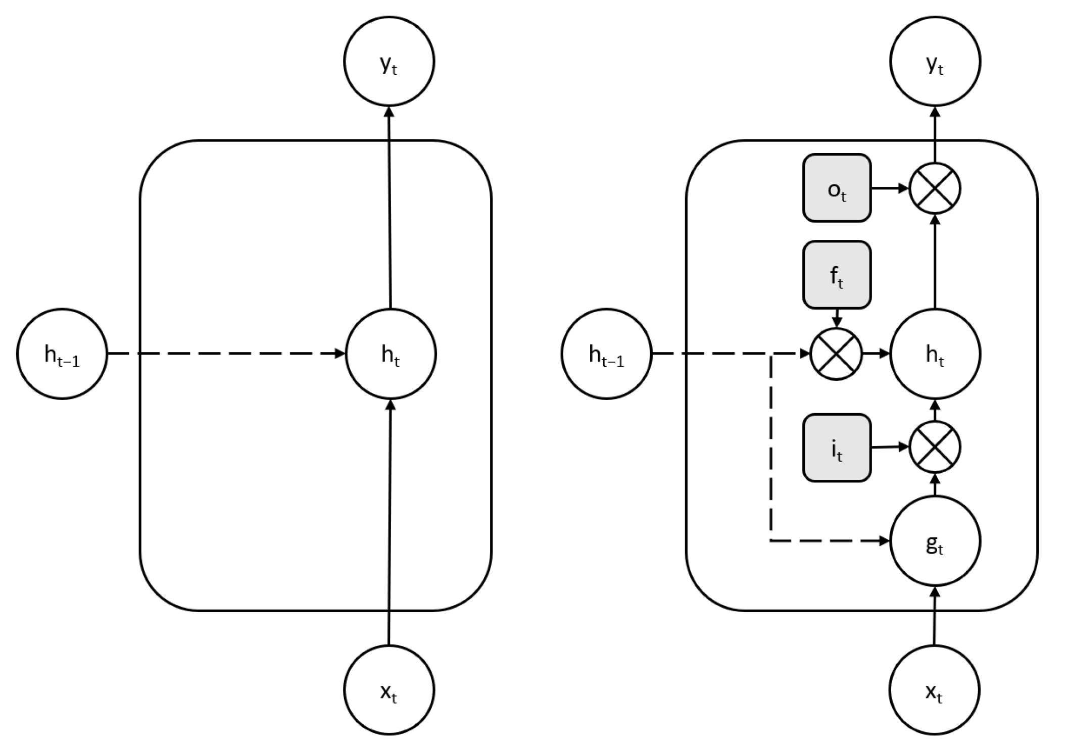
Figure 1. Left: Recurrent neural network (RNN) architecture. Right: Long short-term memory (LSTM) architecture. Dotted lines denote information flow from previous timestep. Grey boxes indicate gate neurons, each of which takes input from the memory cell of the previous timestep ( h t 1 ) and current input state ( x t ). Crossed circles represent elementwise multiplication operations.
Energies 14 00247 g001
Figure 2. Quantile loss function for varying values of τ .
Energies 14 00247 g002
Figure 3. Dropout LSTM model: Log plot of Mean Absolute Error (MAE) loss for 50 training epochs.
Energies 14 00247 g003
Figure 4. GBM model: Log plot of quantile loss for full training phase.
Energies 14 00247 g004
Figure 5. Comparison of observations and predictions for the standard LSTM.
Energies 14 00247 g005
Figure 6. Comparison of observations and predictions with uncertainty estimation for the Bayesian LSTM.
Energies 14 00247 g006
Figure 7. Comparison of observations and predictions with confidence intervals obtained through quantile regression for GBM.
Energies 14 00247 g007
Figure 8. Uncertainty percentage histogram showing the frequency of the uncertainty percentage values in the prediction of January 1999 loads.
Energies 14 00247 g008
Table 1. Configuration parameters for the models (LSTM and XGboost).
ModelConfiguration Parameters
LSTMInput layer, 50 LSTM neurons, 1 neuron output layer
loss (mae), optimizer (adam), epochs (300), batch size (72)
Gradientbooster(gbtree), colsample bytree (1), gamma (0)
Boostinglearning rate (0.1), delta step (0), max depth (3), No estimators (100)
Table 2. European Network on Intelligent Technologies (EUNITE) competition data represented as a multivariate time series.
DatetimeLoadTempertureWeekdayHolidays
1997-01-01 00:30:00797.0−7.5521
1997-01-01 01:00:00794.0−7.5521
1997-01-01 01:30:00784.0−7.5521
1997-01-01 02:00:00787.0−7.5521
1997-01-01 02:30:00763.0−7.5521
Table 3. Evaluation matrix for the three models. MC—Monte Carlo; MAPE—Mean Absolute Percent Error; RMSE—Root Mean Square Error.
LSTMMC DropoutGBR
ModelLSTM ModelModel
MAPE0.0230.0250.023
RMSE18.02518.4817.42
Table 4. Uncertainty correlation with input features used in the prediction of January 1999 load.
LoadTemperatureWeekdayHoliday
−0.050.030.000.00
Publisher’s Note: MDPI stays neutral with regard to jurisdictional claims in published maps and institutional affiliations.