Article

A Data Analytics-Based Energy Information System (EIS) Tool to Perform Meter-Level Anomaly Detection and Diagnosis in Buildings

by
Roberto Chiosa
,
Marco Savino Piscitelli
and
Alfonso Capozzoli
*
Department of Energy “Galileo Ferraris”, TEBE Research Group, BAEDA Lab, Politecnico di Torino, Corso Duca degli Abruzzi 24, 10129 Turin, Italy
*
Author to whom correspondence should be addressed.
Energies 2021, 14(1), 237; https://doi.org/10.3390/en14010237
Submission received: 8 December 2020 / Revised: 28 December 2020 / Accepted: 30 December 2020 / Published: 5 January 2021
(This article belongs to the Special Issue Open Data and Models for Energy and Environment)

Abstract

:
Recently, the spread of smart metering infrastructures has enabled the easier collection of building-related data. It has been proven that a proper analysis of such data can bring significant benefits for the characterization of building performance and spotting valuable saving opportunities. More and more researchers worldwide are focused on the development of more robust frameworks of analysis capable of extracting from meter-level data useful information to enhance the process of energy management in buildings, for instance, by detecting inefficiencies or anomalous energy behavior during operation. This paper proposes an innovative anomaly detection and diagnosis (ADD) methodology to automatically detect at whole-building meter level anomalous energy consumption and then perform a diagnosis on the sub-loads responsible for anomalous patterns. The process consists of multiple steps combining data analytics techniques. A set of evolutionary classification trees is developed to discover frequent and infrequent aggregated energy patterns, properly transformed through an adaptive symbolic aggregate approximation (aSAX) process. Then a post-mining analysis based on association rule mining (ARM) is performed to discover the main sub-loads which mostly affect the anomaly detected at the whole-building level. The methodology is developed and tested on monitored data of a medium voltage/low voltage (MV/LV) transformation cabin of a university campus.

1. Introduction

The building sector is globally recognized as one of the most energy-intensive, and its energy demand continues to increase as a result of a combination of various factors such as extreme climatic events, increased demand for energy services, and in particular those related to air conditioning and quality of the built environment. According to the International Energy Agency (IEA) for the EU member states, buildings are responsible for around 21% of primary energy consumption [1].
As a result, this sector is currently among the most strategic ones for reducing global energy demand, improving energy efficiency, and achieving specific decarbonization targets. In the last years, the great focus on buildings has also been encouraged by the introduction of a robust regulatory framework that puts in evidence the importance of a more responsible building energy management. In this perspective, the technological advancements that characterized the world of IoT (Internet of Things) and ICT (information and communication technology) has played a fundamental role in determining an ever-increasing spread of advanced monitoring and automation infrastructures in buildings, making it is possible to collect a huge amount of data and information related to the real performance in the operation of such complex systems.
The analysis of data collected represents a huge opportunity to identify and define effective energy-saving strategies and to optimize building performance in operation [2,3]. This process can be considered as the starting point of all the activities that are aimed at reducing the gap between the actual and expected building energy performance that is often generated by incorrect occupant behavior, equipment faults, and wrong or ineffective control strategies of energy systems [4].
Moreover, thanks to the growing availability of open access building data sets [5,6,7], analysts can quantitatively compare different processes of analysis, evaluating algorithm performance and assessing building energy performance in a more objective and transparent way [8].
Nonetheless, professional figures involved in the energy management process of buildings are now facing great difficulties in managing these large amounts of data and setting their analyses in a systematic way in order to extract useful knowledge and consequently the desired value.
For this purpose, energy management and information systems (EMISs) can be employed. EMISs belong to the rapidly evolving family of tools that monitor, analyze, and control building energy use and system performance, often leveraging advanced data analytics-based technologies. According to [9], the first classification of EMISs distinguishes such systems considering if their functionalities are enabled at the meter or system-level. The first category of EMISs considers data measurements at a high level (e.g., data related to the total load or of the main sub-loads) while system-level EMISs are focused on more detailed data related to the operation of specific systems or components. energy information systems (EISs) are part of EMIS and integrate software solutions conceived for the analysis of meter-level monitored data of buildings that are not usually collected through building automation systems (BAS). EISs typically enable predictive pattern recognition analysis for performing essential tasks in building energy management such as energy consumption forecasting, anomaly detection and diagnosis, advanced benchmarking, load profiling, and schedule optimization of building energy systems [4].
Among these tasks, anomaly detection and diagnosis has been the most underdeveloped for application on meter-level data.
Anomaly detection and diagnosis (ADD) in buildings is often related to fault detection and diagnosis (FDD) analysis conducted at system/component-level where the scale of analysis is small (e.g., air handling unit components). However, in most real cases, just a few aggregate variables related to the total energy consumption of the building are monitored and collected. Improving the building energy performance by analyzing aggregate data is challenging, especially if several factors such as occupant behavior, comfort levels, operational schedules of systems may generate different energy consumption patterns not always easily inferable. In this context, an EIS tool capable to automatically detect anomalous energy trends in building energy consumption allows energy managers to be promptly informed when the building is not behaving as expected and to avoid inefficient energy management procedures.
In the process of ADD, pattern recognition techniques play a key role in the analysis of patterns and trends in high-dimensional time series of building energy consumption [10]. There are three main expected goals behind ADD analysis in buildings that can be summarised as follows:
  • Identification of typical load patterns in whole-building energy consumption time series.
  • Detection of anomalous load patterns when typical ones are violated over time.
  • Diagnosis of the detected anomalies by means of inference analysis performed on the main sub-loads.
According to the aforementioned objectives, this work proposes an EIS tool capable of performing ADD analysis in buildings by exploiting meter-level data. ADD procedures are usually performed offline and on small subsets of historical data, but more and more interest is growing in developing an automatic framework of analysis for online implementations. For this purpose in this paper, an innovative ADD methodology conceived for application in a real testbed (i.e., the university campus of Politecnico di Torino) is presented. The proposed methodology enables the automatic detection of energy anomalies at the whole-building level and their diagnosis at the sub-load level, revealing which sub-load/sub-loads are responsible for the anomalies detected. According to the objective of this paper, the next paragraph reports and discusses the literature concerning the implementation of ADD processes in buildings and presents the main contributions introduced in this work.

Related Work and Contribution of the Paper

ADD is extremely valuable for improving building energy performance and promising in terms of cost reduction potential if implemented in currently adopted EISs [11]. Despite the great potential offered by ADD at different levels of investigation in buildings, the implementation of this kind of analysis has been majorly focused at the system/component-level (e.g., heating, ventilation, and air conditioning (HVAC) systems), often neglecting applications at whole-building. This trend has been justified by the great availability of system-level data collected by building automation systems (BASs) in buildings. However, extracting any kind of meaningful information from BASs (especially from the outdated ones) can be a complicated task usually characterized by limitations on the data availability. Conversely, the collection of meter-level data in buildings is often performed by means of modern IoT devices that make monitored data easily available as never before. In this context, EIS tools focused on the analysis of meter-level data (especially ADD analysis) are becoming a very fast-growing market in the context of building analytics technologies.
According to the literature, the field of ADD in buildings is progressively leveraging on the application of data analytics techniques [12] for addressing both detection and diagnosis tasks.
The first task is often accomplished through the use of classification, regression, and pattern recognition techniques capable of providing estimations of the building energy consumption in normal operation according to specific boundary conditions (e.g., outdoor climatic conditions). The estimations are then used as a reference baseline for detecting the occurrence of abnormal patterns in the time series that significantly differs from the majority of processed data and/or from the expected trend [13].
For what concerns the implementation of supervised techniques for anomaly detection, in [14] the building energy consumption anomalies are identified comparing the actual consumption with the prediction of a hybrid artificial neural network (ANN) model. A similar approach is adopted in [15], where a deep neural network autoencoder was used to create a prediction model able to successfully detect abnormal energy patterns in the building operational data of an educational building in Hong Kong. Similarly, a general anomaly detection process is also proposed in [16], where the authors employed a variational recurrent autoencoder. Among supervised techniques also classification algorithms proved to be effective in anomaly detection. A robust methodology based on classification trees (CT) was proposed in [17]. In more detail, in that study, a set of classifiers were used for predicting the occurrence of categorical patterns in the time series of the total building electrical load, making it possible to detect a potential anomaly in the case of misclassification (i.e., the same concept of residual analysis in the case of regression models). The study underlined the prediction capabilities of CT algorithms and, most of all, the possibility of exploiting their interpretable nature in anomaly detection problems by extracting useful “if-then” decision rules.
In the context of unsupervised learning for anomaly detection, clustering, and association rule mining (ARM) are the most used techniques [18,19]. In [20], the authors used k-means clustering to automatically discover anomalies in whole-building energy consumption among daily load profiles characterized by an infrequent trend. In [21], an agglomerative hierarchical clustering-based strategy and three different dissimilarity measures were used to identify typical electrical usage profiles that enabled the detection of the abnormal ones.
As previously stated, the use of decision rules in the form of “if-then” implications is extremely valuable in anomaly detection. Following an unsupervised approach, this can be achieved by extracting association rules from building an operational dataset. association rules mining (ARM) algorithms have been widely used to discover abnormal patterns in the energy consumption of buildings and systems and then to enhance their performance. ARM allows discovering causal relationships between events also in the time domain [22]. This kind of algorithm is particularly suitable in extracting hidden knowledge from large databases, as it is reported in [23], where an extensive rules extraction is performed to detect energy wastes in the operation of a lighting system. Similarly, in [10], an improved ARM-based method was employed to discover and detect abnormal operational patterns of HVAC systems installed in a commercial building in Shenzhen (China).
More sophisticated approaches for anomaly detection consist of combining several techniques to maximize the amount of knowledge discovered and automatize the process of analysis.
The study conducted in [24] introduced the concept of collective anomaly detection, described as an event that is considered anomalous only if considered in relation to other events. In the proposed framework, ARM, performed through the Apriori algorithm, was used to extract the most frequent items from a time series related to smart grid operation. Then, anomalous behavior was identified through clustering analysis, considering silhouette indicator as a quality metric. Also, in [25], an anomaly detection process based on an ensembling technique was proposed. In detail, typical building operational patterns were identified by means of clustering analysis, and then an ARM algorithm was used to discover an anomalous load of a cooling chiller system installed in a building in Hong Kong. In [26], a multi-step clustering analysis was performed for removing anomalous daily load profiles from the energy consumption time series of a university campus. Then a regression model was developed on the anomaly-free dataset, combining artificial neural network (ANN) and regression tree (RT), to be used in online applications for detecting the occurrence of anomalous trends in the electrical energy consumption.
Another crucial aspect that arises from the literature review deals with the use of data reduction and transformation methods for (i) reducing the computational cost of the analysis, (ii) easily extracting the main patterns from time series, (iii) improving the effectiveness of supervised and unsupervised algorithms in detecting anomalies. In fact, directly analyzing raw data of time series could be extremely onerous, making difficult the handling and the characterization of the data under investigation. In this perspective, dimensionality reduction can be used with a low computational cost, for example, for removing irrelevant patterns and redundancy from energy consumption datasets. As reviewed in [12], various techniques were explored to enable the classification of data as normal or anomalous, such as principal component analysis (PCA) [27], linear discriminant analysis (LDA) [28], singular variable decomposition (SVD) [29].
In this context, symbolic aggregate approximation (SAX) [30] is one of the most promising techniques available to reduce the size of a time series without losing key information [31]. The SAX algorithm is conceived for the reduction of the time series through a piecewise technique and on its transformation into symbolic strings. Frequent symbolic sub-sequences in the whole sequence can then be extracted and defined as motifs (i.e., normal patterns), while infrequent ones can be isolated and labeled as discords (i.e., potential anomalies). In [31], SAX was used to discover patterns in time series related to the energy consumption of the International Commerce Centre (ICC) in Hong Kong and to recognize inefficient operating conditions that could cause energy wastes. Also, in [20], SAX was used for enabling the extraction of infrequent operating patterns in the energy consumption time series of a school campus and an office building. In particular, discords were detected, setting a minimum frequency threshold to the occurrence of SAX symbol sub-sequences representative of the original daily load profiles. In [17], an enhanced version of SAX called adaptive SAX (aSAX) was used for minimizing the information loss due to the reduction and transformation of energy consumption time series and recognizing motif and discord symbolic patterns by means of classification models.
Once the detection of anomalies in energy consumption is performed, a diagnosis analysis makes it possible to identify the main causes associated with them. The field of anomaly diagnosis has been widely explored in buildings but with a greater focus on system-level applications rather than whole-building level. Also, this research field largely benefits from the use of data analytics techniques following both supervised and unsupervised approaches. The study in [32] proposed a process based on the development of a CT for diagnosing anomalies in the operation of air handling unit (AHU) components. Moreover, in [22], a CT was used for diagnosing up to 11 typical faults in AHU with an accuracy higher than 90%. Indeed, similarly to previously presented studies focused on anomaly detection, also the diagnosis analysis often exploits algorithms that allow the extraction of decision rules. Such a condition is particularly favorable for the final user due to the high interpretability of the diagnosis process, which meaningfulness can then be easily validated by domain expertise. To this aim also ARM algorithms can be employed as reported in [33,34,35,36].
On the basis of the literature review, in most of the cases, only meter level anomaly detection is performed at the whole-building level without any further analysis for identifying anomaly causes among sub-loads at a lower level.
The work presented in this paper aims to bridge this literature gap by introducing a novel hierarchical multi-level approach in the ADD process. The proposed methodology allows to perform the anomaly detection phase at the whole-building level, and only if an anomalous pattern is detected, an event-based diagnostic process is activated for finding root causes at the sub-load level. The event-based hierarchical approach in anomaly diagnosis makes it possible to reduce the computational cost of the analysis and also to rationalize the number and the quality of feedback generated by the ADD tool during operation. Indeed, the final user is not required to visually inspect the trends of all sub-loads in real-time, but he/she is alerted only when interesting events occur, i.e., when specific anomalous conditions among the sub-loads trends generate a divergence of the total load from the expected pattern.
This work combines different advanced data analytics techniques with the aim of maintaining the output of the ADD process human-readable and interpretable while providing accurate results.
The paper considers as a case study the energy consumption data gathered from a monitoring infrastructure installed in the university campus of Politecnico di Torino. The data refer to the electrical energy consumption of a medium voltage/low voltage (MV/LV) transformation cabin that serves different buildings/zones of the campus. In particular, about ten sub-loads of the cabin are available for developing the introduced hierarchical ADD process. The methodology leverages the reduction and transformation of the analyzed time series through an enhanced and adaptive process based on symbolic aggregate approximation (aSAX) as presented in [17]. The aSAX transformation enabled a reduction of the dataset and an effective identification of unexpected operational energy consumption patterns at the sub-daily time windows level. Furthermore, the diagnosis of the abnormal patterns detected at the total load level (i.e., MV/LV transformation cabin) was provided by implementing an association rule mining (ARM) algorithm on the sub-load time series. In this context, the main innovative aspects introduced by the present paper can be summarised as follows:
  • In order to further enhance the pattern recognition process enabled by the aSAX-based process introduced in [17], different features of the energy consumption time series were encoded in symbols in addition to the mean value evaluated in each time window for data reduction purposes. In particular, the encoding of trend features of the time series was performed, allowing an improved characterization of energy consumption behavior and making it possible to reduce the information loss that is always related to the application of temporal abstraction processes such as aSAX. In addition, both the number of time windows and alphabet size for the encoding of the time series in symbols were tuned during the analysis through a fully automatic process.
  • The identification of the normal energy consumption pattern is evaluated for specific time periods during the day (i.e., aSAX time windows) by means of classification models capable of estimating the most probable symbol encoded through the aSAX-based process. In particular, globally optimal evolutionary trees were used to accomplish this task. The use of evolutionary trees introduce a twofold advantage in the classification task: (i) the results obtained from their application are fully interpretable as they can be translated in “if-then” decision rules, (ii) the achievable accuracy in high-dimensional problems can be significantly higher than the performance of standard decision trees (e.g., locally optimal classification trees [37]).
  • The anomaly diagnosis is performed at the sub-load level by implementing an unsupervised data analytics technique based on an ARM algorithm. The diagnostic process is capable of automatically updating an anomaly library in the form of “if-then” association rules extracted from historical data. This opportunity allows the developed ADD tool to evolve during building operation, significantly increasing its generalizability.
  • The whole methodology was conceived for being applied in a real testbed paying attention to its generalizability and scalability to other buildings. In this perspective, the developed ADD process is capable of self-tuning its hyper-parameters ensuring a robust performance in online implementations. As a reference, the algorithms for both detection and diagnosis of the energy anomalies can be easily retrained periodically or considering an event-based approach (e.g., the occurrence of a not pre-identified anomaly).
The rest of the paper is organized as follows. Section 2 provides an overview and a brief theoretical description of the data analytics methods used for conducting ADD analysis. Section 3 presents and describes the case study considered for the analysis. Section 4 introduces the methodological framework on the basis of the ADD analysis performed. Eventually, Section 5 and Section 6 presents and discusses the results obtained, while in Section 7, the concluding remarks and future research perspectives are reported.

2. Description of the Data Analysis Methods

In this section, the data analytics methods employed in this work are briefly described. The method description is not intended to be exhaustive, but it is aimed to underline the usefulness in the framework of this study and building energy data exploitation.

2.1. Adaptive Symbolic Aggregate Approximation (aSAX)

Meter-level data measurements are collected in the so-called time series: a two-dimensional matrix where each row corresponds to a single observation in time and the column to a measured variable [31]. The sampling frequency determines the time interval between two consecutive observations, and for building applications, it is usually in the order of minutes. As a consequence, the resulting high-dimensional time series is often computationally expensive to be stored and analyzed in its original form. In this context, many dimensionality reductions and transformation techniques were proposed in the literature; one of the most widely used is the symbolic aggregate approximation (SAX), which makes it possible to compress time series while preserving its fundamental characteristics [30]. This process segments the original time series in sub-sequences, each of them is summarised with a single numerical value (e.g., mean value) that is then encoded into the alphabetic symbol and finally combined into a string. The resulting string is much shorter than the original time series and enables the application of various pattern recognition techniques while reducing the computational cost. In the last years, some variations to the original algorithm have been proposed in the literature, especially with the aim of generalizing some initial assumptions (e.g., data distribution) and facing information loss issues always generated from the reduction and transformation of time series. In the author’s opinion, one of the greatest improvements to the SAX was introduced through the so-called adaptive symbolic aggregate approximation (aSAX) [38]. In the following, the main steps of aSAX process are presented, with specific reference to their implementation in the present work.
  • Chunking: The original time series (y(t) = {y1, … yn}) of length n is divided into N non-overlapping sub-sequences (T = {T1, … TN}) chosen for the specific context. In the case of energy consumption time series, the selection of the length of the sub-sequences is influenced by the periodicity of the energy pattern observed, and for building applications, it is usually set to 24 h. Each sub-sequence is further divided into W segments called time windows (τ = {τ1, … τW}). The parameter W is word size. During this process, it is possible to choose time windows with equal or different length, based on user preference [17,39];
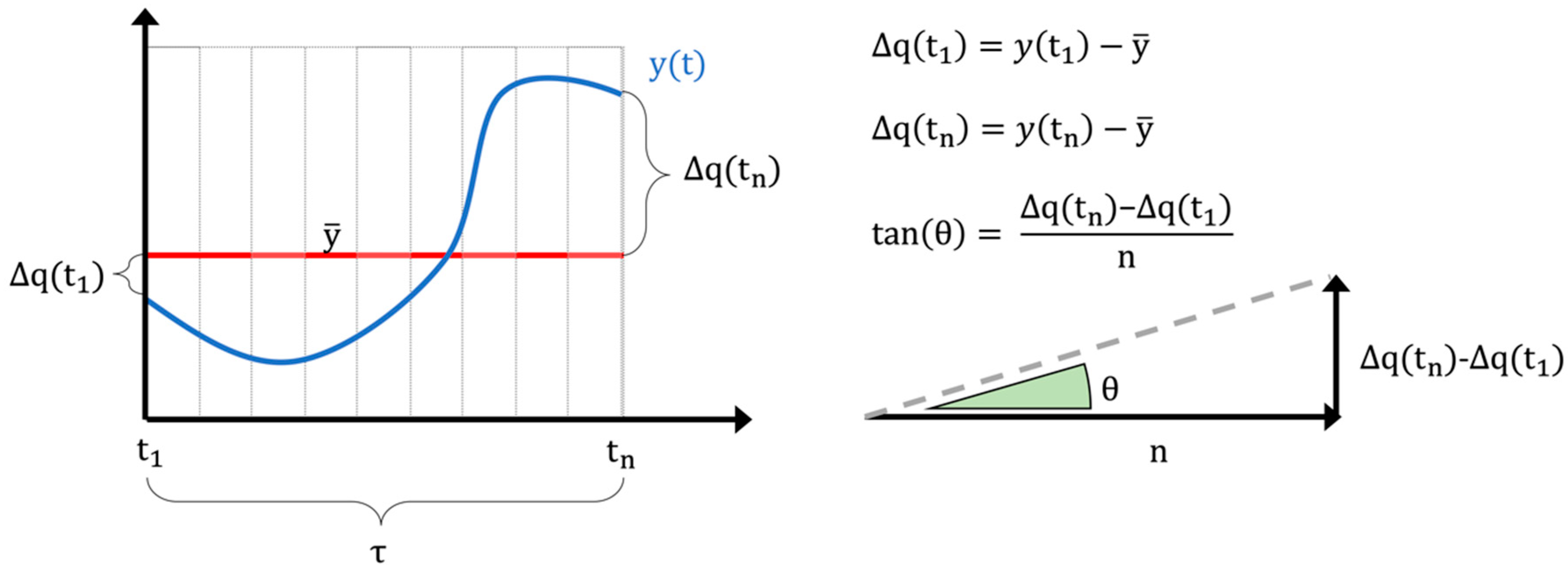
  • Feature extraction: In this step, an aggregated numerical feature is calculated starting from the sub-sequence of the original time series that falls in the generic time window τi, and this value is considered as representative of all the data points included in that window. Aggregated features can extract some important characteristics of the time series while losing some other information. The analyst chooses which feature is the most significant and whether one or more features are needed for the purpose of the study. The most used and known approach is called piecewise aggregate approximation (PAA), which performs a constant approximation of the original time series y(t) by replacing the values that fall into the same time window τ with their mean [40]. Many other statistical features can be extracted (mean, variance, kurtosis, skewness) not only from the time domain but even from other domains such as the frequency one [41]. A feature representing important characteristics of time series is, for example, the trend angle [42]. This feature is particularly effective in describing the time series trend, and it was employed in this study. In detail, given a time series y(t) = {y1, … yn} of length n in a given time window τ = {t1, … tn}, defined ∆q(t1) and ∆q(tn) the first order distance between the initial and final point with the time series mean, can be defined a trend triangle as shown as in Figure 1. The trend angle feature θ, green in Figure 1, is defined with the following equation:
θ = atan ( Δ q ( t n ) Δ q ( t 1 ) n )
Figure 1. Definition of trend feature triangle and trend angle for a generic time series (y(t)).
Energies 14 00237 g001
The trend angle domain ranges continuously from −90° to 90°. If the trend angle value is approximately zero (θ ≈ 0), the trend is stationary; if it is positive (θ > 0), the trend is rising; vice versa if it is negative (θ < 0), the trend is descending.
  • Encoding: this step consists of setting an alphabet size α and assigning an alphabetic character to each time window, according to where the extracted numerical feature lies within a set of breakpoints (β = {β1, … βα-1}) identified according to the shape of the feature distribution. The aSAX algorithm [38] finds the optimal positions of breakpoints through an iterative process by minimizing the distance among all the data points included between two consecutive breakpoints and their centroid (calculated average center). Eventually, the symbol can be assigned for each window (τ), creating a word of length W for the given sub-sequence (Ti). The original numerical time series y(t) is then transformed into an alphabetic string (y(α)) of length W∗N.
Figure 2 shows an example of time series temporal abstraction conducted with the aSAX process. An electrical load time series (y(t) = {y1, … y192} (black line)) with a 15 min sampling frequency, is divided into two sub-sequences Ti and Ti+1 of 24 h each. In this example, five-time windows (W = 5) of unequal length are identified for each sub-sequence, and the alphabet size is set to five (α = 5), meaning that four breakpoints β = {β1, β2, β3, β4} are identified. The time series is then approximated through PAA (red segments), and for each segment, the corresponding symbol is assigned. The PAA values distribution is shown on the right side of the figure in red and the breakpoints, evaluated through the aSAX, in dashed blue lines. The original time series for the time window (Ti+1) is converted from a numerical vector into an alphabetic string “a-b-d-c-a”, reducing it from a 96-dimensional object to a 4-dimensional one.

2.2. Recursive Partitioning and Globally Optimal Evolutionary Tree

Classification is the task of assigning a class label to unlabelled data instances through a classifier model, providing prediction or description of a given dataset [43]. The classification model is created through an inductive learning algorithm using a training set, which is a data frame with attributes and labeled instances. Once the model has been created, its performance is evaluated on a test set through the comparison between the predicted and real labels. The decision tree is the most commonly used model for classification, thanks to its understandable graphical representation. Depending on the type of target attribute, discrete categorical or continuous numerical, a decision tree is called, either a classification tree or regression tree, respectively. The tree consists of a root, internal nodes, and leaves, all connected by branches. The construction of a tree classifier can be performed through different algorithms; in this framework, recursive partitioning and globally optimal evolutionary tree are considered.
The most commonly used recursive partitioning method is the classification and regression tree (CART), which is a binary decision tree based on the splitting of the instances in purer subsets (i.e., nodes) through decision rules [44]. It proceeds in a forward step-wise approach by maximizing homogeneity in each child node, yielding to a local optimal tree.
Conversely, the so-called evolutionary decision tree is based on a stochastic algorithm that aims to construct a globally optimum classification model [37]. This process randomly initializes the root node split, then at each iteration, variation operators (i.e., split, prune, major split rule mutation, minor split rule mutation, crossover) are applied. The survivor is selected, and the process is repeated until the stopping criterion is satisfied. The evolutionary tree algorithm used in this paper is implemented in the R package “evtree” [37].
One of the most important hyper-parameter that can be set for this algorithm is the variation operator probability, which refers to the probability that a given variation operator is chosen at a generic iteration. The default operator probability considered is c20m40sp40, meaning that the algorithm has a 20% probability of selecting the crossover operator, a 40% probability for selecting one of the mutation operators (20% for minor split rule mutation and 20% for major split rule mutation) and a 40% probability for selecting one of the split (with 20% probability) or the prune operators (with 20% probability).
The advantage of an evolutionary tree algorithm is that it tends to offer higher accuracy in prediction than recursive partitioning algorithms [37] while maintaining the same interpretable tree structure.

2.3. Association Rules Mining (ARM)

ARM is a widely used technique that allows extracting static causal relationships and correlations between attributes in a dataset. The objective is to find a group of variables (items) that frequently occur together in a database. This technique can only handle categorical variables, and it is usually computationally costly. One of the most used ARM algorithms is the iterative Apriori algorithm based on a frequent itemset that allows the extraction of static rules from a categorical transactional dataset [45]. Association rules are defined between a set of items (or itemset) in the form A ⇒ B, where A is the itemset called antecedent (LHS = left-hand side of the rule) and B consequent (RHS = right-hand side of the rule) and A ∩ B = ∅. Rule extraction is usually restricted to only an item in the consequent.
Some user-defined parameters (confidence, support, and lift) need to be set in order to evaluate the significance of the obtained rules and filter out the less important. A domain expert sets those parameters according to each specific case. The support is calculated as the probability of the intersection between the antecedent A and consequent B (supp(A ⇒ B) = P(A ∩ B)), expressing the co-occurrence of the two events. The confidence (conf(A ⇒ B) = P(B|A)), defined as the conditional probability between A and B, allows assessment of the reliability of a rule. It gives the probability of the consequent event in all transactions containing the antecedent. The lift is the ratio between the confidence and support of consequent B (lift(A ⇒ B) = P(B|A) / P(B)). When the lift is higher than 1, it means that B is positively correlated with A, while if the lift is lower than 1, it suggests a negative correlation; otherwise, if the lift is equal to 1, there is no correlation at all. This parameter is particularly important since it allows one to select the most interesting rules [31]. In this paper, the ARM Apriori algorithm was used to extract interesting associations between the total building load and its sub-loads, especially during events detected as anomalous. This data analytics method was perfectly integrated with the outcome of the aSAX and classification processes, of which the results consist of categorical values.

3. Case Study

The case study analyzed refers to the energy consumption of a MV/LV transformer cabin identified as “substation C”, that serves a part of the main campus of Politecnico di Torino (PoliTo), an Italian university located in Turin. Data related to the total electrical load and to some sub-loads are available with 15 min timesteps from 1 January 2015 to 31 December 2019. The hierarchical structure of the available data is shown in Figure 3: the first level refers to the total electrical load of substation C, while the second level shows the available sub-loads. In addition, the load breakdown in terms of average annual energy consumption was provided.
In particular, a bar and a canteen were at the disposal of students and campus staff and accounted for 2.75% and 16.03%, respectively, of the total electrical energy consumption of substation C. The university data center accounted for 13.16% of the total energy consumption. The administration offices (rectory) corresponded to 3.83% of energy consumption and the mathematics department (DIMAT) for 2.21%. A large share of energy consumption (12.22%) was related to the mechanical room. The equipment located in this room included hot and chilled water circuits and auxiliaries such as recirculation pumps. The chilled water was provided by two chillers of nominal electrical power of 220 kW and a rated cooling capacity of 1120 kW, and a reversible water-water heat pump, with nominal a power and cooling capacity of 165 kW and 590 kW, respectively.
The remaining energy consumption was aggregated under a unique instance tagged as “Unlabelled_load” as showed in Figure 3. It accounted for 48.76% of the total energy consumption, and since it was not directly measured, cannot be assigned to a specific sub-load.

4. Methodological Framework

In this section the conceived ADD methodology is presented and described. The proposed methodology aims to develop a two-level ADD analysis capable of making in a first step a high-level detection on total electrical load time series (at meter level) and in a second step performing the anomaly diagnosis on sub-loads (at sub-meter level). The methodology follows the flow chart structure shown in Figure 4.
In particular, four steps of analysis are considered.
  • Pre-processing: The first step consists of pre-processing data that was aimed at removing punctual anomalies and inconsistencies from the datasets. The dataset used in this study included electrical load data (collected from substation C) from 1 January 2015 to 31 December 2019 with a 15 min sampling frequency. Negative measurements were removed a priori. Nearly-zero values of electrical load related to continuously operating systems (refrigerators, emergency lighting) were considered inconsistent and removed. Statistical outliers (e.g., data affected by transmission problems) were also identified and removed by means of boxplot analysis. Then all statistical inconsistencies and missing values are replaced through a linear interpolation;
  • Temporal abstraction of the time series: In the second step of the analysis, the temporal abstraction of the electrical load time series was performed according to the procedure introduced in [17]. Temporal abstraction consists of the reduction and transformation of the time series in a sequence of alphabetic symbols. In particular, a recursive partitioning regression tree (RT) was used to identify sub-daily time windows with an unequal length for dimensionality reduction, considering the total electrical load from 2015 to 2019 as a numerical target and the hours of the day as a predictive attribute, as performed in [17]. Once time windows were evaluated, the PAA approximation is performed. The breakpoint identification was carried out through the aSAX method procedure by choosing the appropriate alphabet size through a k-means clustering process. The identification of the optimal number of clusters (i.e., alphabet size) was implemented through the R package “NbClust” [46];
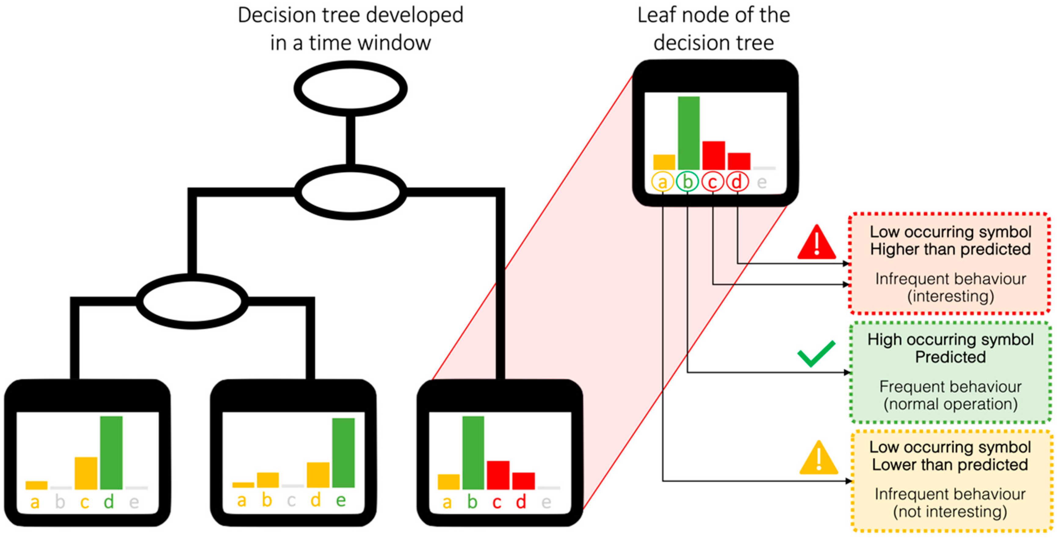
  • Anomaly detection at total electrical load level: Anomaly detection was performed on the encoded total electrical load time series of substation C. In each sub-daily time window, the total electrical load symbol obtained through aSAX was predicted through a globally optimal evolutionary tree [37], using as explanatory attributes contextual information such as calendar variables (day type and holiday) and energy variables (electrical demand of sub-loads). The model was developed through a test-train-validation process and was able to predict the expected symbol in each time widow with high accuracy. However, when the model failed to correctly predict the symbol in a time window, the occurrence of a potential anomaly was assumed. Referring to Figure 5, the predicted symbol is the one with the higher occurrence in a given leaf node (green bar). All other symbols were infrequent and then potentially anomalous (yellow and red bars). Given the interest in detecting higher electrical load than normal, only the tree leaves nodes that showed infrequent symbols corresponding to a high electrical load (red bars in Figure 5) were considered and investigated in the following diagnostic phase;
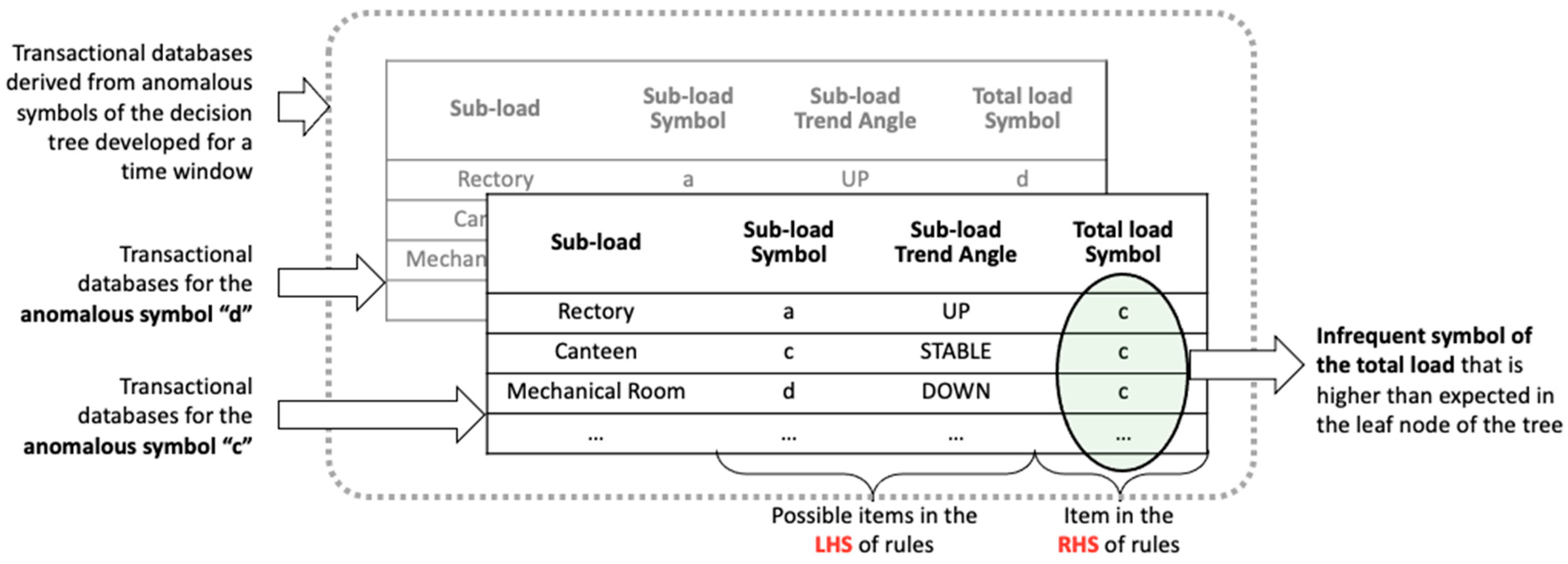
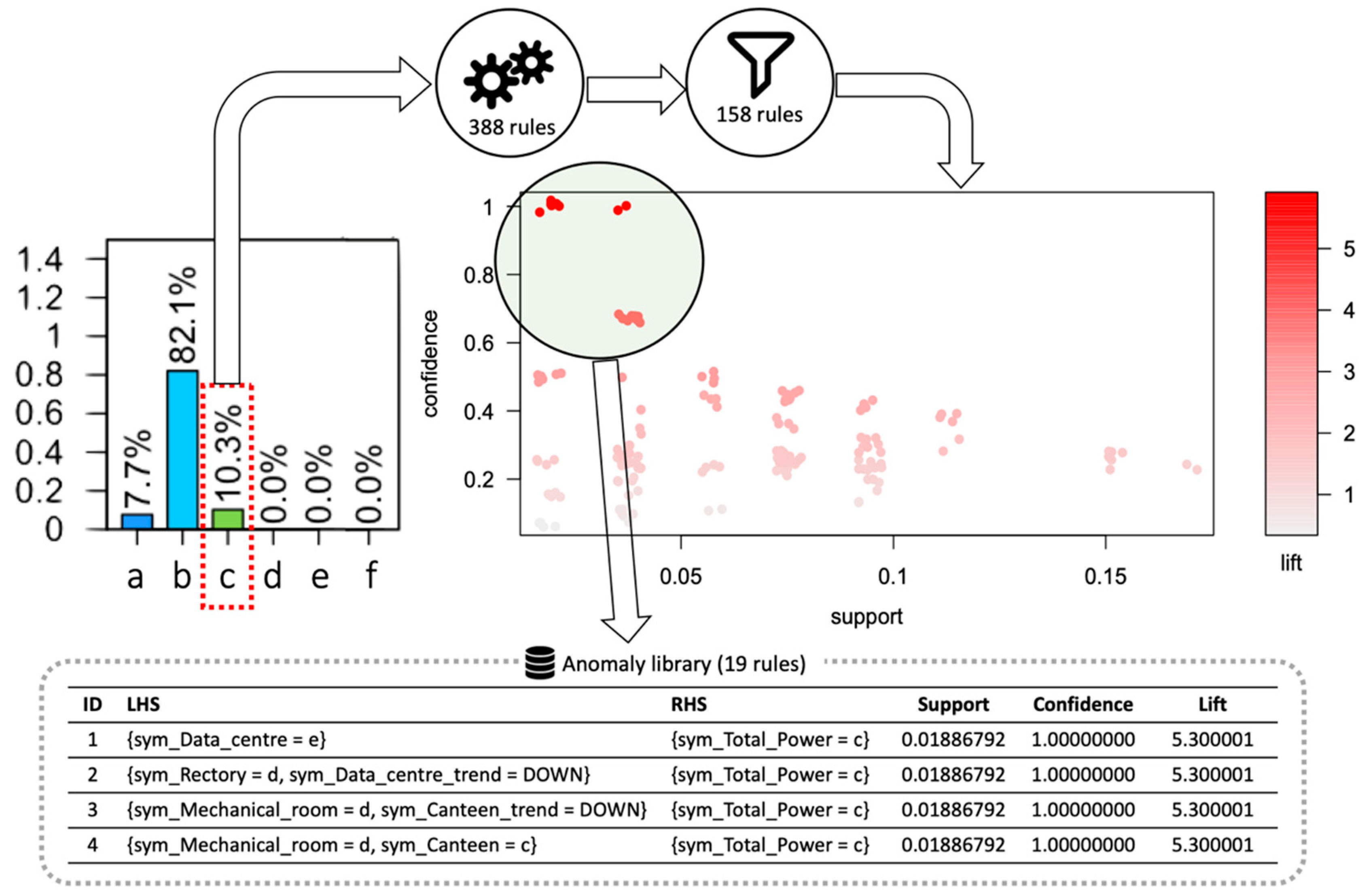
  • Diagnosis at sub-load level: Once the classification models were developed, a post-mining phase was performed. The post-mining phase was aimed at searching historical relationships between misclassified total electrical load symbols and specific trends of sub-loads occurred in same time window. The process is described in Figure 6. The anomalous symbols identified in the training phase of the models were extracted and stored in a categorical data frame (Step-1 in Figure 6). From time series of sub-loads, the mean value and the trend angle were extracted. They were categorised through the aSAX process and then added to the categorical data frame (Step-2 in Figure 6). This data frame was then transformed into a transactional database on which ARM was applied (Step-3 in Figure 6). The LHS is composed of the additional categorical variables related to sub-loads, while RHS contains only the total electrical load anomalous symbol. ARM automatically extracts a set of rules which connects the historical infrequent behaviour of the total electrical load with the sub-load conditions. This process was implemented through the R package “arules” [47]. Resulting rules were then sorted and filtered setting appropriate interest measures parameters such as support, confidence and lift (Step-4 in Figure 6). Filtered rules were then stored within an anomaly library where they were ranked to show which sub-load condition (for example high electrical load or significantly uptrend) was responsible for the anomalous total electrical load behaviour. The tool gives a critical insight of the historical energy behaviour and, when implemented in real time load analysis, can provide useful feedback on which energy management actions are needed.

5. Results

The previously described methodology was applied to the case study presented in Section 3. The quantitative analysis of data was performed through the statistical software R [48], and results related to each stage are reported in the following sections.

5.1. Pre-Processing

The pre-processing phase allowed to handle missing values and to remove outliers. The procedure was applied to the total electrical load and sub-loads dataset.
In particular, punctual outliers due to data transmission problems were detected, removed, and replaced through linear interpolation. The carpet plots of the total electrical load of substation C are reported in Figure 7a (one for each year considered). It can be seen that the building energy systems were usually turned on at 6:00 and turned off at 19:00. The electrical load increased from the night baseload until 8:00 when teaching activities and office activities began and started decreasing after 16:00. This pattern was visible for every working day (from Monday to Friday) with an average electrical load (from 8:00 to 16:00) of more than 300 kW. During the weekend, on the other hand, there was a significant decrease in the average electrical load to 100 kW, mainly due to the weekly university break and the absence of teaching and office activities. The same carpet plot representation is reported in Figure 7 for some representative sub-loads. Figure 7b shows the electrical load of the mechanical room in the years from 2015 to 2019. Because of the intensive use of the chillers in summer, the highest monthly average electrical load was reached in July with a value of about 100 kW. During the winter months, the electrical load was not zero because of the electrical demand of the recirculation pumps. Figure 7c shows the electrical load of the campus canteen. Also, this load is strongly dependent on the weekly university occupancy schedule. In fact, a significant decrease in the average electrical load was visible during weekends, when the campus was unoccupied, and no teaching or office activity took place.

5.2. Time Series Abstraction

In order to perform the data transformation and dimensionality reduction, the original time series of the electrical load was split into 24 h intervals since a daily periodical pattern was observed.
The time windows of daily load profiles were evaluated through a RT, considering the total electrical load as a numerical target and the hours of the day as a predictive attribute. The total electrical load from 2015 to 2019 was analyzed.
Holidays and weekends were excluded from the analysis since they usually present profiles that are flat or with low variance, and include those days in the model would have reduced the accuracy of the results. The splitting criterion adopted was based on the variance reduction around the numerical target’s mean in each leaf node. In this way, the daily pattern was split into homogeneous consumption time windows. As a stopping criterion, a minimum number of objects in the child nodes at each split was set in order to have a time window length of at least 2 h.
The RT automatically identified the optimal number of windows thanks to a cost complexity pruning process. This procedure allowed us to choose the best tree by generating a fully expanded tree and then prune it iteratively. According to [17], this procedure enables the identification of an optimal trade-off between misclassification error and model complexity. The selection of the optimal tree size was performed according to the one standard error rule (i.e. 1-SE rule) [49].
The resulting tree had five leaves, which corresponded to five sub-daily time windows, which are summarised in Table 1. It can be seen that the first and fifth-time windows corresponded to the night hours during which the university was closed and not occupied. On the opposite, the remaining time windows correspond to occupied hours of the campus.
Once the time windows were identified, the PAA was performed in order to prepare the dataset for the encoding through the aSAX process.
A fundamental parameter to be set in the aSAX process is the alphabet size (α), which determines how many symbols are going to be used for the encoding, and as a consequence, also the number of breakpoints to search. While in the literature, the alphabet size is usually selected according to domain expertise [17,20,31], in this framework, an unsupervised technique consisting of k-means partitive clustering was used. In particular, the reduced data of the time series (through PAA) were clustered in order to find homogeneous groups and determine the optimal number of breakpoints. For this purpose, during the clustering process, several cluster quality indices, embedded in the R package NbClust [46], were calculated in order to assess the optimal number of clusters (k) according to a majority rule approach, setting a search space between k = 3 and k = 8. The results obtained suggested the partition with k = 6 as the optimal one, then determining the setting of the alphabet size value also equal to 6.
In detail, the positions of breakpoints, calculated under equally probability assumption, were used as initialization of the aSAX iterative algorithm [38]. As shown in Figure 8, those breakpoints (dotted lines) were not able to divide the distributions effectively, producing narrow intervals at low values and wider intervals for higher values of the reduced PAA time series. The final adaptive breakpoints (solid lines) were evaluated once a tolerance of 1010 on the representation error was reached (after about 60 iterations).
Figure 9 shows the carpet plot and histograms, referring to the encoded total electrical load time series. In particular, Figure 9a shows that in the first and fifth-time window, the most frequent symbols were “a” and “b”, which corresponded to a low electrical load during night hours. In the second and fourth-time windows, corresponding to early morning and late afternoon, there was a prevalence of medium electrical load identified with the symbol “d” describing the switch-on/off of the systems. In the third time window, the symbols “e” and “f” were the most frequent since the electrical load in the middle of the day is the highest.
Figure 9b shows the histograms of electrical load symbols divided by time windows and years. From this representation was evident how the load patterns had changed during the years from 2015 to 2019. In particular, in the first and fifth-time windows, a change of pattern from the symbol “b” to the symbol “a” was visible due to a lower baseload during night hours, when the campus was unoccupied. This behavior could be related to the refurbishment of buildings and/or systems served by substation C. The same trend was seen in the third time window where a change of pattern from the symbol “f” to the symbol “e” was visible, resulting in a lower electrical load during peak hours. This behavior suggests that the energy performance of the campus was improving over time. Further considerations about changes in the load patterns of the campus have been made in the following when the selection of a proper training period for the classification models is discussed.

5.3. Anomaly Detection at Total Electrical Load Level

For each time window, a globally optimal evolutionary tree was developed in order to further investigate the dependency of the total electrical load (i.e., target variable) from the boundary conditions (i.e., predictive variables).
To create a model that automatically learns new patterns as the building energy consumption changes, a training period that is consistent with the recent past was selected. In fact, as previously discussed, older patterns of energy consumption strongly differed from more recent ones, and including them in the learning training set could have compromised the capabilities of the models in terms of accuracy on the validation set. Therefore, the classification models were trained and tested on 2018 data and for simulating an online deployment of the process were validated on the first month of 2019. In particular, the 2018 dataset was split, with 80% placed into the train set and 20% into the test set, through a random sampling process.
The attributes considered in the evolutionary classification trees are listed in the following:
  • Day type: input ordinal categorical variable representative of each day of the week with values from 1 (Monday) to 7 (Sunday);
  • Holiday: input binary categorical variable YES/NO capable of distinguishing working from non-working days;
  • Total Power pre: mean total electrical load (in kW) calculated in the previous time window to the one considered for the classification (numerical input variable);
  • Canteen: mean electrical load (in kW) of the canteen calculated in the time window considered for the classification (numerical input variable);
  • Mechanical room: mean electrical load (in kW) of the mechanical room calculated in the time window considered for the classification (numerical input variable);
  • Symbol: target categorical variable representative of the encoded symbol of the total electrical load in a time window.
The choice to use as predictive values some sub-loads and not others was driven by a sensitivity analysis and by their percentage weight on the total electrical load. The canteen and the mechanical room weights were 12.22% and 16.03%, respectively, on the total electrical load (Figure 3). Moreover, among the labeled sub-loads, they showed the highest variance in 2018, as well as significant variations during the day. It is clear how they could be extremely useful in characterizing the relationships that existed between the normal operation of the substation C and their electrical demand.
For all the time windows, the maximum depth of the classification tree was set to 6, the minimum number of observations in each node was set to 20, and the default setting c20m40sp40 for variation operators was assumed (20% crossover, 40% mutation, and 40% split/prune).
Since the evolutionary algorithm and the splitting process were randomly initialized, the seed for the random number generator was set in the code in order to replicate the analysis easily.
Figure 10 shows the tree resulting from the training phase for the second time window. It shows that it effectively classified in each leaf node the most frequent symbol from the others while maintaining a readable and understandable structure. The developed set of evolutionary trees (one for each time window) was aimed at extracting very accurate decision rules so that in the leaf node, a high occurring symbol can be found. If this condition is satisfied, the low occurring symbols can be considered as potential anomalies for the considered time window. Those potential anomalies could then be subject to further investigation in order to understand which sub-load can be assumed as the cause for that infrequent behavior (anomaly diagnosis).
Decision rules extracted from each tree (one for each time window) are reported in Table 2. It can be observed that the input variables used for the classification tree were able to explain the occurrence of each symbol with strong accuracy. Furthermore, it can be noticed that time window one was not associated with any decision rule. This window was found to be characterized by a very high occurrence (over 97% over the training period) of a single symbol. In this case, the available input variables were not able to further characterize the occurrence of other symbols.
The model performance for each time window is shown in Table 3. The table also reports that the overall accuracy in training testing and validation was 88.91%, 86.22%, and 89.03%, respectively. The results obtained suggest high generalizability for the classification models and the absence of overfitting issues.

5.4. Diagnosis at Sub-Load Level

Once the classification models were created, the subset of anomalous symbols (higher than expected symbols) included in each node was transformed into a transactional database that contains the categorical target variable (total electrical load symbol) and some additional explanatory variables related to the sub-loads.
To extract those additional categorical variables, the sub-loads were subjected to the same time series abstraction process described for the total electrical load in Section 5.2. Using the same time window discretization as the total electrical load and the same alphabet size (α = 6), each time series of the available sub-loads was encoded through the aSAX process.
In order to further enrich information about sub-loads, the trend angle was also extracted and encoded (see Figure 11).
This feature allows tracking of the trend of the time series in each time window, making it possible to know if the load is increasing, decreasing, or it is stable. In this case, the alphabet size was set to three (α = 3) in order to reflect those three possible trends (respectively encoded as Up, Down, and Stable). The initial breakpoints, calculated under equally probability assumption, were used as initialization of aSAX iterative algorithm, and the final adaptive breakpoints were evaluated once a tolerance of 10−10 on the representation error was reached. Then the Apriori ARM algorithm was applied to the transactional database structured, as depicted in Figure 12.
In particular, the RHS was the anomalous total electrical load symbol extracted from the leaf node of the classification tree for a specific time window, while the LHS was composed of all possible combinations of electrical load symbols and trend angles symbols of sub-loads. The minimum and the maximum number of items in a transaction was set in order to obtain rules with one or maximum of two items in the LHS. The minimum support to mine rules was set to 0.005, and the minimum confidence to 0.005. Redundant rules, equally or less predictive of a more general rule with the same confidence [50], were removed, and the remaining ones were represented in a scatter plot (Figure 13). The scatter plot helps the analyst to understand how interesting rules were filtered out by setting lift(A ⇒ B) > 1 and conf(A ⇒ B) > 0.5. Those rules were then stored in the anomaly library, where they were ranked according to the lift value. LHS of those rules represents the sub-load conditions that were found to be significantly influencing the abnormal total electrical load.
An example of the procedure is shown in Figure 13 for node five of the second time window. In this node, the most frequent symbol was “b”, and the only infrequent interesting symbol (higher electrical load) was “c”. The transactional database was then constructed: the LHS was composed of the additional categorical variables related to sub-loads (electrical load symbol and trend angle symbol), while RHS contained only the total electrical load anomalous symbol (symbol “c”). ARM automatically extracts 338 rules, of which 180 resulted redundantly, and 158 rules were significant. After filtering, only 19 rules were stored in the anomaly library. In this particular case, the most frequent items in the anomaly library were: mechanical room symbol “d”; canteen symbol “c”; rectory symbol “d”. For example, among the 19 rules considered, rule four (IF sym_Mechanical_room = “d” AND sym_Canteen = “c” ⇒ sym_Total_Power = “c”) had a lift value of about five and confidence of 100%. It means that if during the operation of the ADD process this rule was matched, then the diagnosis was extremely robust, given that the anomaly detected was already present in the analyzed historical database.

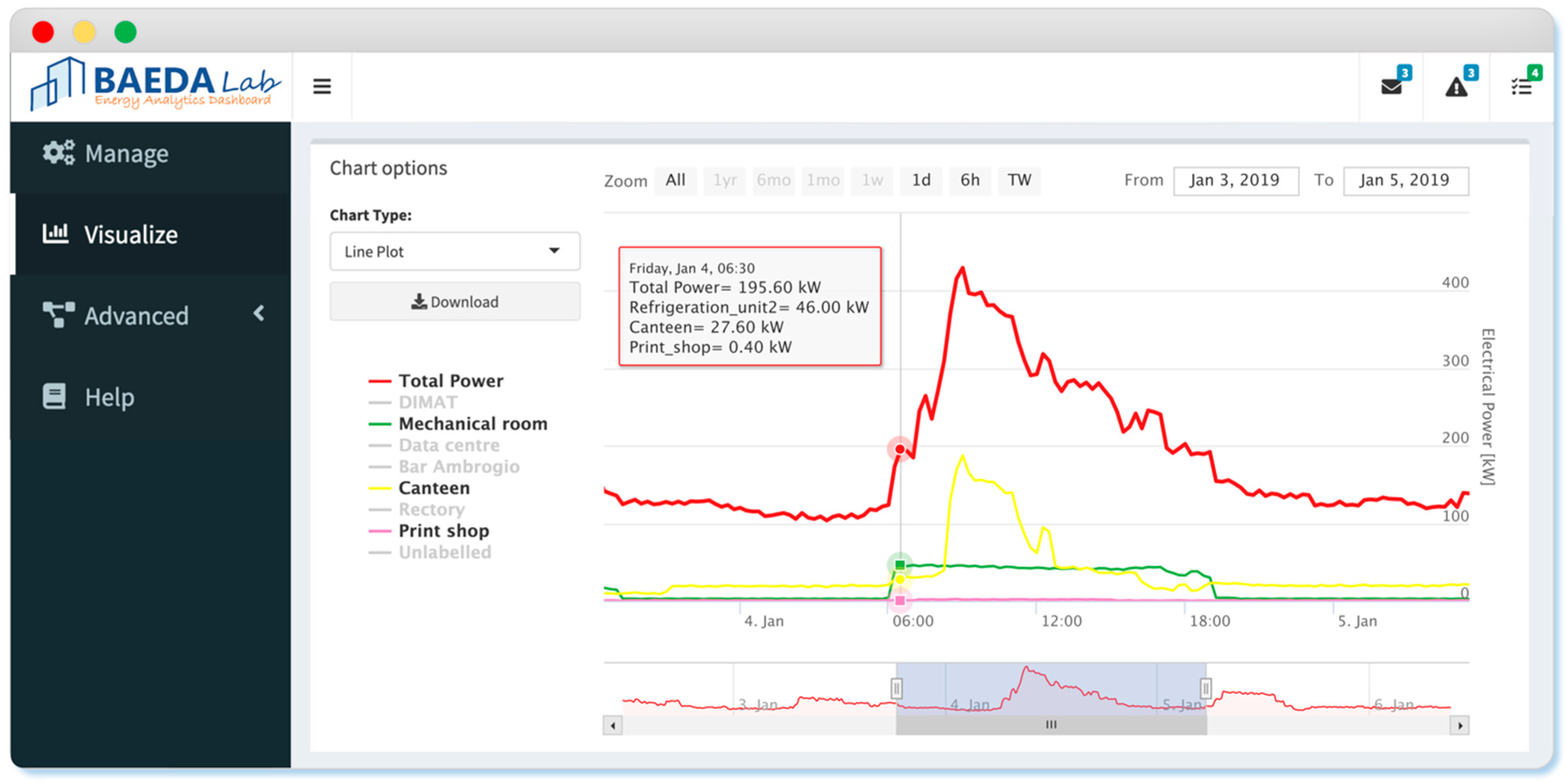
5.5. Deployment of the ADD Tool

The methodology was conceived to be implemented in a real-time data acquisition tool connected to a smart metering infrastructure. The metering infrastructure continuously collects data, and once a time window ends, the symbol of the total electrical load was calculated through aSAX and compared to the one predicted by the globally optimal tree. Three possible cases could then occur:
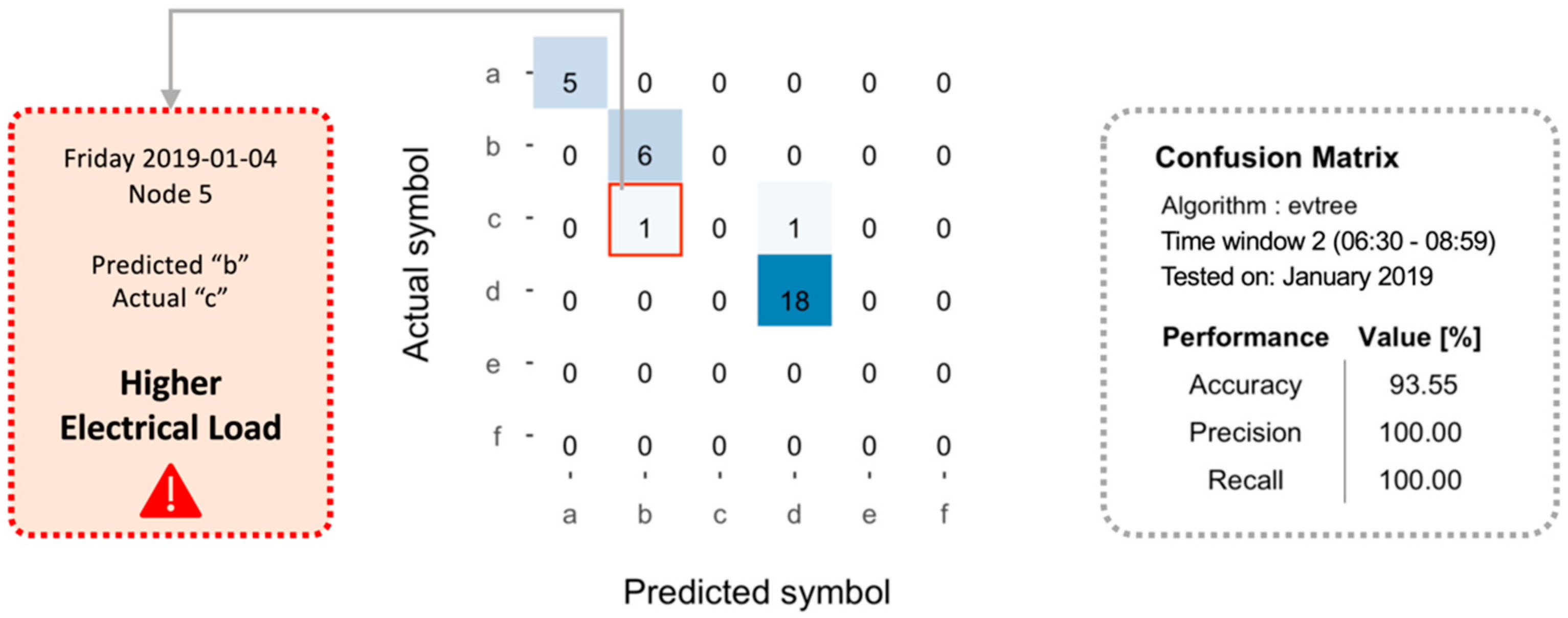
  • The actual symbol was the same as the predicted one. This means that given the boundaries conditions, the total electrical load of that time window is behaving as expected, then no further diagnosis is requested;
  • The actual symbol was different from the predicted symbol and indicated a lower electrical load than expected. This means that even though the total electrical load of that time window is not behaving as expected, no further diagnosis is required. This is due to the focus of the methodology for which an anomaly is related only to higher consumption than expected;
  • The actual symbol was different from the predicted symbol and indicated a higher electrical load than expected. This means that given the boundaries conditions, the total electrical load of that time window is higher than expected, and then a further investigation is needed.
In the latter case, the diagnosis analysis is enabled. Given the boundary conditions, the corresponding leaf node of the evolutionary tree is identified, and the tool automatically retrieves the library of association rules extracted on the historical dataset for that specific anomaly condition (i.e., a specific symbol of the total electrical load). The following step was then to extract the additional features from sub-loads and encoding them in symbols/categorical values. Once all the potential LHS items had been computed, a scan of the rules included in the anomaly library was performed to detect any perfect match. If a perfect match of a rule exists, it means that a full diagnosis of the anomaly could be performed considering that the same anomaly condition (i.e., the relation between anomalous total load and sub-loads) was present in the historical dataset. Otherwise, if a perfect match does not exist, a partial match with the single item was searched. In the case of a partial match, the diagnostic capability is not as strong as for the perfect rule match. However, useful insight can be obtained about new possible configurations of sub-loads that could be included in the anomaly library during future updates. In order to make the whole ADD process flexible in learning new patterns, a full retraining of the classification models and anomaly library is supposed to be performed every month, considering a historical dataset of one year.
The deployment of the methodology was performed on the validation set that consisted of the data referred to in January 2019. The process of detection through the evolutionary tree was performed on all-time windows. Only for reference, it was considered the classification performance achieved in the second time window for the whole month. The confusion matrix related to the classifier is reported in Figure 14. In particular, it can be seen that the classification tree achieved an accuracy of 93.55%, and only one time the actual symbol was different from the predicted one revealing a higher electrical load than expected, respectively “c” instead of “b”. In particular, the anomaly occurred on 4 January 2019.
Once identified the day and the time window of the anomaly, the corresponding tree’s leaf node was identified as well. In the example, the anomalous symbol of the total electrical load of 4 January 2019 was detected in the tree leaf node five. The diagnosis process was then enabled, and the sub load conditions were compared with the anomaly reference library. In the considered example, there was not a perfect rule match but a partial one on the following items:
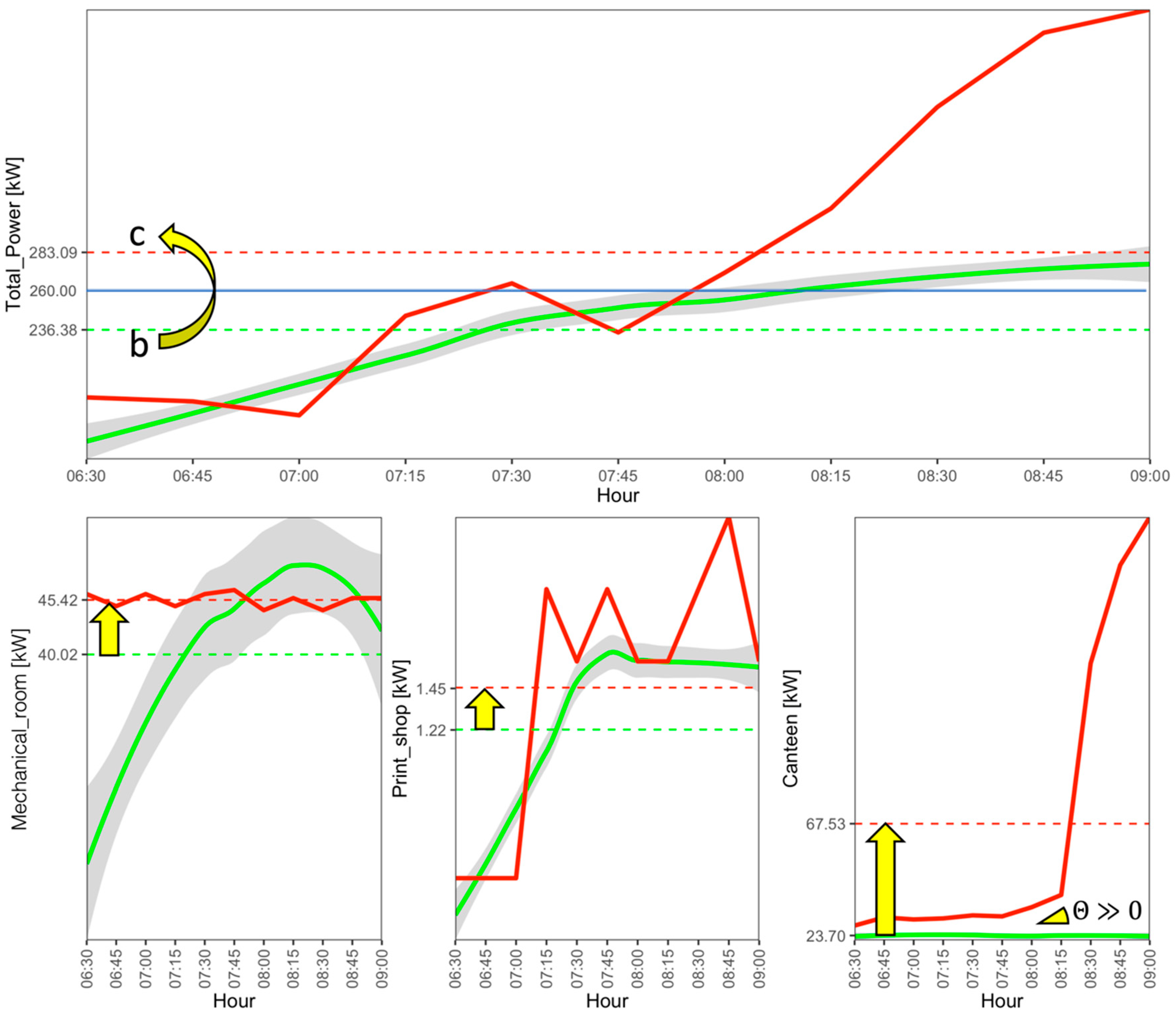
  • Printshop electrical load symbol “c”.
  • Mechanical room electrical load symbol “c”.
  • Canteen electrical load symbol “c”.
  • Canteen trend angle symbol “UP”.
As previously discussed, a partial match is not as strong as a perfect rule match but provides useful suggestions to be considered for conducting the anomaly diagnosis. This aspect was demonstrated through further graphical analysis, reported in Figure 15. The figure shows a comparison between the anomalous and normal pattern of the total electrical load and the loads related to the mechanical room, printshop, and canteen. Only the second time window is reported in the plot. In particular, in red, the anomalous data related to the 4 January 2019 are reported, while in green are shown the frequent “normal” patterns of the given loads extracted from the training period (part of 2018). Along with the actual electrical loads (solid lines) were reported the relative PAA segments (dashed lines) and, for the “normal” pattern, the standard deviation (grey areas).
The combined effect of the three sub-loads (i.e., mechanical room, printshop, canteen) led to an overall electrical load higher than expected. The mean total electrical load rose from 236 kW (symbol “b”) to 283 kW (symbol “c”), and it was easy to verify that the identified sub-loads contributed almost 90% to the power shift upward of the total electrical load. It is worth noting that although the printshop presented an anomalous electrical load pattern, the observed profile (red line) did not significantly deviate from the normal one (green line).

6. Discussion of the Results

This paper focused on the development of ADD methodology able to analyze meter-level electrical load data in order to detect anomalous patterns and perform a diagnosis process on sub-loads. This methodological framework was conceived to be highly scalable and reliable in order to be implemented in energy data monitoring infrastructure for supporting a prompt detection of anomalies avoiding energy wastes over time.
The time window size and alphabet size for the aSAX encoding are key parameters. In [20] is reported an interesting sensitivity analysis based on these two parameters, showing that a trade-off between window numbers and alphabet size has to be found in order to minimize the variance between patterns and resolution needed. In this paper, the time window number was chosen by using an RT and the alphabet size by a k-means clustering evaluation. Once those parameters are set, the aSAX encoding procedure can be considered completely automatic. Moreover, the conducted analysis showed that considering the trend angle as an additional feature, a robust sub-loads characterization could be performed without adding computational burden.
Moreover, the selection of the predictive variables for the globally optimal classification tree needs particular attention. The overall energy consumption of a building is strongly related to the occupancy schedule, environmental conditions, thermo-physical features of the building, and the behavior of users. For this reason, those variables should be all included in the classification model and could help in describing infrequent but non-anomalous patterns. On the other hand, trustworthy values are difficult to retrieve or measure with continuity. Surely, the inclusion of those variables could qualitatively increase the model predictions.
A further interesting aspect of being considered is related to the data that should be used for training and how often training is needed. It is well known that building electrical load varies over the years due to the electrification of end-uses and the seek of the higher performance of appliances and facilities. For this reason, a good trade-off between retraining rate and computational effort should be performed. In our study, we validated the model in the first month of 2019 in order to assess its accuracy.
In addition, in order to prove the effectiveness of monthly retraining of the tool, a comparison was performed between two different deployment approaches. The first deployment considered was static, with the hypothesis of using the same classification models trained in 2018 for six months in 2019. The second deployment was dynamic, considering monthly retraining of the classification models with a one-year moving window training set. Results showed that the average classification accuracy was 82.85% for the dynamic deployment and was 78.77% for the static one. Therefore, with a dynamic deployment, the anomaly detection capabilities improved, given that the classifiers are able to learn new patterns that change over time. Following the same reasoning, the authors propose to implement a monthly update also for the association rules included in the anomaly library.

7. Conclusions and Future Work

This paper proposed a multiple-step ADD methodology to automatically detect at whole-building meter level anomalous energy consumption and then perform a diagnosis on the sub-loads responsible for that anomalous pattern. Frequent and infrequent electrical load patterns, properly transformed through an adaptive symbolic aggregate approximation process, were discovered by means of globally optimum evolutionary classification trees. Association rule mining was employed to discover the main sub-loads, which mostly affected the anomaly detected at the whole-building level.
In the future, the ADD process presented in this paper is expected to be implemented online within the energy information system of Politecnico di Torino and supplied through an energy data analytics dashboard developed with the R packages “shiny” [51] and “shinydashboard” [52]. Figure 16 reports a demo of the dashboard that is currently under construction and under offline testing. Moreover, the authors aim to integrate this ADD process together with other complementary tools able to perform electrical load forecasting and energy performance tracking (i.e., benchmarking).
Further research will also be focused on the testing of alternative configurations of algorithms (i.e., data clustering, forecasting) with respect to the one considered in this study. In fact, the proposed algorithms cannot always be assumed as the best solution for performing such kind of analysis on energy consumption time series. As a reference, the aSAX transformation, the development of classification trees, and the extraction of association rules perfectly match with the need to provide a fully interpretable tool to the final user. However, this constraint, in some cases, can also determine an information loss and accuracy decrease. For this reason, a future analysis may well consider the use of more sophisticated algorithms (e.g., deep learning algorithms) that are characterized by their non-interpretable nature but makes it possible to achieve higher performance in detecting and diagnosing energy anomalies. This option still remains valuable if an explanation layer is included in the analytical process. Nowadays, such a task corresponds to the main goal of the machine learning field of the so-called explainable artificial intelligence (XAI), which offers new opportunities for effectively embedding advanced algorithms in AI-based energy management solutions where explanations of the black-box model predictions are often compulsory.

Author Contributions

Conceptualisation, M.S.P. and A.C.; Data curation, M.S.P.; Formal analysis, R.C.; Investigation, M.S.P.; Methodology, M.S.P., R.C. and A.C.; Project administration, A.C.; Software, R.C.; Supervision, A.C.; Validation, M.S.P. and A.C.; Writing—original draft, R.C.; Writing—review and editing, M.S.P. and A.C. All authors have read and agreed to the published version of the manuscript.

Funding

This research received no external funding.

Institutional Review Board Statement

Not applicable.

Informed Consent Statement

Not applicable.

Data Availability Statement

The data presented in this study are available on request from the corresponding author. The data are not publicly available due to privacy restrictions related to a part of the dataset and the absence of a proper data management platform.

Acknowledgments

The authors express their gratitude to the Living Lab of Politecnico di Torino for providing data and to Giovanni Carioni for the support in data preparation and collection.

Conflicts of Interest

The authors declare no conflict of interest.

References

  1. IEA. Buildings A Source of Enormous Untapped Efficiency Potential. Available online: https://www.iea.org/topics/buildings (accessed on 7 September 2020).
  2. Fan, C.; Yan, D.; Xiao, F.; Li, A.; An, J.; Kang, X. Advanced data analytics for enhancing building performances: From data-driven to big data-driven approaches. Build. Simul. 2020. [Google Scholar] [CrossRef]
  3. Capozzoli, A.; Mechri, H.E.; Corrado, V. Impacts of architectural design choices on building energy performance applications of uncertainty and sensitivity techniques. In Proceedings of the IBPSA 2009 International Building Performance Simulation Association, Glasgow, Scotland, 27–30 July 2009; pp. 1000–1007. [Google Scholar]
  4. Capozzoli, A.; Cerquitelli, T.; Piscitelli, M.S. Enhancing Energy Efficiency in Buildings Through Innovative Data Analytics Technologies. In Pervasive Computing; Elsevier: Amsterdam, The Netherlands, 2016; ISBN 9780128037027. [Google Scholar]
  5. Miller, C.; Meggers, F. The Building Data Genome Project: An open, public data set from non-residential building electrical meters. Energy Proc. 2017, 122, 439–444. [Google Scholar] [CrossRef]
  6. Miller, C.; Kathirgamanathan, A.; Picchetti, B.; Arjunan, P.; Park, J.Y.; Nagy, Z.; Raftery, P.; Hobson, B.W.; Shi, Z.; Meggers, F. The Building Data Genome Project 2, energy meter data from the ASHRAE Great Energy Predictor III competition. Sci. Data 2020, 7, 1–13. [Google Scholar] [CrossRef] [PubMed]
  7. Attanasio, A.; Piscitelli, M.S.; Chiusano, S.; Capozzoli, A.; Cerquitelli, T. Towards an automated, fast and interpretable estimation model of heating energy demand: A data-driven approach exploiting building energy certificates. Energies 2019, 12, 1273. [Google Scholar] [CrossRef] [Green Version]
  8. Manfren, M.; Nastasi, B.; Groppi, D.; Astiaso Garcia, D. Open data and energy analytics—An analysis of essential information for energy system planning, design and operation. Energy 2020, 213, 118803. [Google Scholar] [CrossRef]
  9. Kramer, H.; Lin, G.; Granderson, J.; Curtin, C.; Crowe, E. Synthesis of Year One Outcomes in the Smart Energy Analytics Campaign Building Technology and Urban Systems Division; Lawrence Berkeley National Laboratory: Berkeley, CA, USA, 2017. [Google Scholar]
  10. Zhang, C.; Zhao, Y.; Li, T.; Zhang, X. A post mining method for extracting value from massive amounts of building operation data. Energy Build. 2020, 223. [Google Scholar] [CrossRef]
  11. Fan, C.; Sun, Y.; Shan, K.; Xiao, F.; Wang, J. Discovering gradual patterns in building operations for improving building energy efficiency. Appl. Energy 2018, 224, 116–123. [Google Scholar] [CrossRef]
  12. Himeur, Y.; Ghanem, K.; Alsalemi, A.; Bensaali, F.; Amira, A. Anomaly detection of energy consumption in buildings: A review, current trends and new perspectives. arXiv 2020, arXiv:2010.04560. [Google Scholar]
  13. Esling, P.; Agon, C. Time-series data mining. ACM Comput. Surv. 2012, 45. [Google Scholar] [CrossRef] [Green Version]
  14. Chou, J.S.; Telaga, A.S. Real-time detection of anomalous power consumption. Renew. Sustain. Energy Rev. 2014, 33, 400–411. [Google Scholar] [CrossRef]
  15. Fan, C.; Xiao, F.; Zhao, Y.; Wang, J. Analytical investigation of autoencoder-based methods for unsupervised anomaly detection in building energy data. Appl. Energy 2018, 211, 1123–1135. [Google Scholar] [CrossRef]
  16. Pereira, J.; Silveira, M. Unsupervised Anomaly Detection in Energy Time Series Data Using Variational Recurrent Autoencoders with Attention. In Proceedings of the 17th IEEE International Conference on Machine Learning Applications ICMLA, Orlando, FL, USA, 17–20 December 2018; pp. 1275–1282. [Google Scholar] [CrossRef]
  17. Capozzoli, A.; Piscitelli, M.S.; Brandi, S.; Grassi, D.; Chicco, G. Automated load pattern learning and anomaly detection for enhancing energy management in smart buildings. Energy 2018, 157, 336–352. [Google Scholar] [CrossRef]
  18. Capozzoli, A.; Piscitelli, M.S.; Brandi, S. Mining typical load profiles in buildings to support energy management in the smart city context. Energy Proc. 2017, 134, 865–874. [Google Scholar] [CrossRef]
  19. Zhao, Y.; Zhang, C.; Zhang, Y.; Wang, Z.; Li, J. A review of data mining technologies in building energy systems: Load prediction, pattern identification, fault detection and diagnosis. Energy Built Environ. 2020, 1, 149–164. [Google Scholar] [CrossRef]
  20. Miller, C.; Nagy, Z.; Schlueter, A. Automated daily pattern filtering of measured building performance data. Autom. Constr. 2015, 49, 1–17. [Google Scholar] [CrossRef]
  21. Li, K.; Yang, R.J.; Robinson, D.; Ma, J.; Ma, Z. An agglomerative hierarchical clustering-based strategy using Shared Nearest Neighbours and multiple dissimilarity measures to identify typical daily electricity usage profiles of university library buildings. Energy 2019, 174, 735–748. [Google Scholar] [CrossRef]
  22. Piscitelli, M.S.; Mazzarelli, D.M.; Capozzoli, A. Enhancing operational performance of AHUs through an advanced fault detection and diagnosis process based on temporal association and decision rules. Energy Build. 2020, 226, 110369. [Google Scholar] [CrossRef]
  23. David, M.C.; Zareipour, H. Data association mining for identifying lighting energy waste patterns in educational institutes. Energy Build. 2013, 62, 210–216. [Google Scholar] [CrossRef]
  24. Rossi, B.; Chren, S.; Buhnova, B.; Pitner, T. Anomaly Detection in Smart Grid Data: An Experience Report. In Proceedings of the 2016 IEEE International Conference on Systems, Man, and Cybernetics (SMC), Budapest, Hungary, 9–12 October 2016; pp. 2313–2318. [Google Scholar]
  25. Xiao, F.; Fan, C. Data mining in building automation system for improving building operational performance. Energy Build. 2014, 75, 109–118. [Google Scholar] [CrossRef]
  26. Piscitelli, M.S.; Brandi, S.; Capozzoli, A.; Xiao, F. A data analytics-based tool for the detection and diagnosis of anomalous daily energy patterns in buildings. Build. Simul. 2020, 1–17. [Google Scholar] [CrossRef]
  27. Imayakumar, A.A.; Dubey, A.; Bose, A. Anomaly Detection for Primary Distribution System Measurements using Principal Component Analysis. In Proceedings of the 2020 IEEE Texas Power and Energy Conference (TPEC), College Station, TX, USA, 6–7 February 2020; pp. 1–6. [Google Scholar]
  28. Zhang, L.; Wan, L.; Xiao, Y.; Li, S.; Zhu, C. Anomaly Detection method of Smart Meters data based on GMM-LDA clustering feature Learning and PSO Support Vector Machine. In Proceedings of the 2019 IEEE Sustainable Power and Energy Conference (iSPEC), Beijing, China, 20–24 November 2019; pp. 2407–2412. [Google Scholar]
  29. Khoshrou, A.; Pauwels, E.J. Data-driven pattern identification and outlier detection in time series. Adv. Intell. Syst. Comput. 2019, 858, 471–484. [Google Scholar] [CrossRef] [Green Version]
  30. Lin, J.; Keogh, E.; Wei, L.; Lonardi, S. Experiencing SAX: A Novel Symbolic Representation of Time Series. Data Min. Knowl. Discov. 2007, 15, 107–144. [Google Scholar]
  31. Fan, C.; Xiao, F.; Madsen, H.; Wang, D. Temporal knowledge discovery in big BAS data for building energy management. Energy Build. 2015, 109, 75–89. [Google Scholar] [CrossRef]
  32. Yan, R.; Ma, Z.; Zhao, Y.; Kokogiannakis, G. A decision tree based data-driven diagnostic strategy for air handling units. Energy Build. 2016, 133, 37–45. [Google Scholar] [CrossRef]
  33. Liu, J.; Shi, D.; Li, G.; Xie, Y.; Li, K.; Liu, B.; Ru, Z. Data-driven and association rule mining-based fault diagnosis and action mechanism analysis for building chillers. Energy Build. 2020, 216, 109957. [Google Scholar] [CrossRef]
  34. Tightiz, L.; Nasab, M.A.; Yang, H.; Addeh, A. An intelligent system based on optimized ANFIS and association rules for power transformer fault diagnosis. ISA Trans. 2020, 103, 63–74. [Google Scholar] [CrossRef] [PubMed]
  35. Huang, R.; Liu, J.; Chen, H.; Li, Z.; Liu, J.; Li, G.; Guo, Y.; Wang, J. An effective fault diagnosis method for centrifugal chillers using associative classification. Appl. Therm. Eng. 2018, 136, 633–642. [Google Scholar] [CrossRef]
  36. Zhang, T.; Lu, J.; Zhang, G.; Ding, Q. Fault diagnosis of transformer using association rule mining and knowledge base. In Proceedings of the 2010 10th International Conference on Intelligent Systems Design and Applications, Cairo, Egypt, 29 November–1 December 2010; pp. 737–742. [Google Scholar]
  37. Grubinger, T.; Zeileis, A.; Pfeiffer, K.P. Evtree: Evolutionary learning of globally optimal classification and regression trees in R. J. Stat. Softw. 2014, 61, 1–29. [Google Scholar] [CrossRef] [Green Version]
  38. Pham, N.D.; Le, Q.L.; Dang, T.K. HOT aSAX: A Novel Adaptive Symbolic Representation for Time Series Discords Discovery. In Lecture Notes in Computer Science; (including subseries Lecture Notes in Artificial Intelligence and Lecture Notes in Bioinformatics); Springer: Berlin, Germany, 2010; Volume 5990, pp. 113–121. ISBN 3642121446. [Google Scholar]
  39. Keogh, E.; Chakrabarti, K.; Pazzani, M.; Mehrotra, S. Locally adaptive dimensionality reduction for indexing large time series databases. In Proceedings of the 2001 ACM SIGMOD International Conference on Management of Data, Santa Barbara, CA, USA, 21–24 May 2001; pp. 151–162. [Google Scholar]
  40. Keogh, E.; Chakrabarti, K.; Pazzani, M.; Mehrotra, S. Dimensionality Reduction for Fast Similarity Search in Large Time Series Databases. Knowl. Inf. Syst. 2001, 3, 263–286. [Google Scholar] [CrossRef]
  41. Zhang, Y.; Duan, L.; Duan, M. A new feature extraction approach using improved symbolic aggregate approximation for machinery intelligent diagnosis. Meas. J. Int. Meas. Confed. 2019, 133, 468–478. [Google Scholar] [CrossRef]
  42. Yu, Y.; Zhu, Y.; Wan, D.; Liu, H.; Zhao, Q. A novel symbolic aggregate approximation for time series. Adv. Intell. Syst. Comput. 2019, 935, 805–822. [Google Scholar] [CrossRef]
  43. Tan, P.-N.; Steinbach, M.; Karpatne, A.; Kumar, V. Cluster Analysis: Basic Concepts, and Algorithms. In Introduction to Data Mining; Pearson: London, UK, 2019; p. 526. [Google Scholar]
  44. Piscitelli, M.S.; Brandi, S.; Capozzoli, A. Recognition and classification of typical load profiles in buildings with non-intrusive learning approach. Appl. Energy 2019, 255, 113727. [Google Scholar] [CrossRef]
  45. Aggarwal, C.C. Data Data Mining: The Textbook; Springer: Berlin, Germany, 2012. [Google Scholar]
  46. Charrad, M.; Ghazzali, N.; Boiteau, V.; Niknafs, A. NbClust: An R Package for Determining the. J. Stat. Softw. 2014, 61, 1–36. [Google Scholar] [CrossRef] [Green Version]
  47. Michael, H.; Buchta, C.; Gruen, B.; Hornik, K.; Johnson, I.; Borgelt, C. Package ‘ arules ’: Mining Association Rules and Frequent Itemsets Description; R Foundation for Statistical Computing: Vienna, Austria, 2020; pp. 1–109. [Google Scholar]
  48. R Core Team. R: A Language and Environment for Statistical Computing; R Foundation for Statistical Computing: Vienna, Austria, 2017. [Google Scholar]
  49. Atkinson, E.J.; Therneau, T.M. An Introduction to Recursive Partitioning Using the RPART Routines. Mayo Clin. Sect. Biostat. Tech. Rep. 2000, 61, 33. [Google Scholar]
  50. Hahsler, M.; Chelluboina, S. Visualizing Association Rules: Introduction to the R-extension Package arulesViz. In R Project Module; R Foundation for Statistical Computing: Vienna, Austria, 2011; pp. 1–24. [Google Scholar]
  51. Chang, W.; Cheng, J.; Allaire, J.; Xie, Y.; McPherson, J. Package ‘ shiny ’: Web Application Framework for R; R Foundation for Statistical Computing: Vienna, Austria, 2020; p. 238. [Google Scholar]
  52. Chang, W.; Ribeiro, B.B. Package “ShinyDashboard”: Create Dashboards with “Shiny”. J. Stat. Softw. 2018, 14, 1–27. [Google Scholar]
Figure 2. Example of an adaptive symbolic aggregate approximation (aSAX) process applied to an electrical load time series (T = 24 h, W = 5, α = 5).
Energies 14 00237 g002
Figure 3. Hierarchical structure of the electrical load database under study.
Energies 14 00237 g003
Figure 4. Flow chart explaining the adopted methodology.
Energies 14 00237 g004
Figure 5. Interpretation of anomaly detection results.
Energies 14 00237 g005
Figure 6. Sub-meter level diagnosis methodology description.
Energies 14 00237 g006
Figure 7. Carpet plot of the (a) total electrical load (substation C) (b) mechanical room (c) canteen.
Energies 14 00237 g007
Figure 8. Step by step identification of adaptive breakpoints through the aSAX algorithm applied to the total electrical load.
Energies 14 00237 g008
Figure 9. aSAX representation of the total electrical load: (a) carpet plots (b) histogram distributions of symbols along the time windows and years.
Energies 14 00237 g009
Figure 10. Globally optimum classification tree for the second time window (06:30–08:59).
Energies 14 00237 g010
Figure 11. Results of trend angle aSAX encoding applied to the rectory sub-load: (a) identification of adaptive breakpoints through the aSAX algorithm, (b) encoded trend angle carpet plot for 2018 and 2019.
Energies 14 00237 g011
Figure 12. Representation of the transactional databases used for the extraction of association rules. LHS: left-hand side of the rule; RHS: right-hand side of the rule.
Energies 14 00237 g012
Figure 13. Diagnosis procedure of extracting, filtering, and selecting only relevant association rules from node five of the second time window.
Energies 14 00237 g013
Figure 14. Confusion matrix for the globally optimal classification tree predicting January 2019 total electrical load symbol in the 2nd time window. Red square: the detected anomalous behavior.
Energies 14 00237 g014
Figure 15. Comparison between the actual (red lines) and expected (green lines) electrical load with the relative standard deviation (grey areas) on 4 January 2019. The dashed green and red lines represent the PAA segments for the actual and expected load respectively. The blue horizontal solid line on the top graph represents the aSAX breakpoint related to the total power.
Energies 14 00237 g015
Figure 16. Energy data analytics dashboard developed by the building automation and energy data analytics (BAEDA) Lab, which implements the anomaly detection and diagnosis (ADD) procedure presented in this paper.
Energies 14 00237 g016
Table 1. Sub-daily time windows for total electrical load.
IDTime WindowDuration
100:00–06:296 h 30 min
206:30–08:592 h 30 min
309:00–15:446 h 45 min
415:45–19:143 h 30 min
519:15–23:594 h 45 min
Table 2. Decision rules extracted from globally optimal trees created in each time window on the training period.
Time WindowNodeDecision RuleSymbolAccuracy
00:00–06:291-⇒ a97.3%
06:30–08:592IF Holiday = Yes⇒ a92.0%
5IF Holiday = No AND Mechanical room < 85.84 kW AND Canteen < 96.4 kW⇒ b82.1%
6IF Holiday = No AND Mechanical room < 85.84 kW AND Canteen ≥ 96.4 kW⇒ d89.7%
8IF Holiday = No AND Mechanical room ≥ 85.84 kW AND Canteen < 108.4 kW⇒ c71.4%
9IF Holiday = No AND Mechanical room ≥ 85.84 kW AND Canteen ≥ 108.4 kW⇒ e86.5%
09:00–15:443IF Canteen < 54.4 kW AND Holiday = Yes⇒ a96.0%
5IF Canteen < 54.4 kW AND Holiday = No AND Total Power pre < 257.1 kW⇒ b76.5%
6IF Canteen < 54.4 kW AND Holiday = No AND Total Power pre ≥ 257.1 kW⇒ c85.0%
8IF Canteen ≥ 54.4 kW AND Canteen < 143.5 kW⇒ e73.9%
10IF Canteen ≥ 143.5 kW AND Mechanical room < 38 kW⇒ e86.0%
11IF Canteen ≥ 143.5 kW AND Mechanical room ≥ 38 kW⇒ f81.1%
15:45–19:142IF Total Power pre < 388.8 kW⇒ a87.4%
4IF Total Power pre ≥ 388.8 kW AND Total Power pre < 614 kW⇒ d86.5%
5IF Total Power pre ≥ 388.8 kW AND Total Power pre ≥ 614 kW⇒ d85.4%
19:15–23:592IF Holiday = Yes⇒ a96.0%
4IF Holiday = No AND Day Type = {6,7}⇒ a97.2%
6IF Holiday = No AND Day Type = {1,2,3,4,5} AND Canteen < 16.5 kW⇒ a85.5%
7IF Holiday = No AND Day Type = {1,2,3,4,5} AND Canteen ≥ 16.5 kW⇒ b87.6%
Table 3. Accuracy results from a comparison between test and validation.
Time WindowTraining
(80% 2018)
Test
(20% 2018)
Validation
(Jan. 2019)
00:00–06:2997.30%96.89%100%
06:30–08:5987.33%82.19%93.55%
09:00–15:4483.56%79.45%58.06%
15:45–19:1486.64%86.30%96.77%
19:15–24:0089.72%86.30%96.77%
Mean88.91%86.22%89.03%
Publisher’s Note: MDPI stays neutral with regard to jurisdictional claims in published maps and institutional affiliations.

