Article

A Time Series Sustainability Assessment of a Partial Energy Portfolio Transition

Department of Engineering Management and Systems Engineering, Missouri University of Science and Technology, Rolla, MO 65409, USA
*
Author to whom correspondence should be addressed.
Energies 2021, 14(1), 141; https://doi.org/10.3390/en14010141
Submission received: 1 December 2020 / Revised: 21 December 2020 / Accepted: 24 December 2020 / Published: 29 December 2020
(This article belongs to the Special Issue Integrated Approaches for Enterprise Sustainability)

Abstract

:
Energy portfolios are overwhelmingly dependent on fossil fuel resources that perpetuate the consequences associated with climate change. Therefore, it is imperative to transition to more renewable alternatives to limit further harm to the environment. This study presents a univariate time series prediction model that evaluates sustainability outcomes of partial energy transitions. Future electricity generation at the state-level is predicted using exponential smoothing and autoregressive integrated moving average (ARIMA). The best prediction results are then used as an input for a sustainability assessment of a proposed transition by calculating carbon, water, land, and cost footprints. Missouri, USA was selected as a model testbed due to its dependence on coal. Of the time series methods, ARIMA exhibited the best performance and was used to predict annual electricity generation over a 10-year period. The proposed transition consisted of a one-percent annual decrease of coal’s portfolio share to be replaced with an equal share of solar and wind supply. The sustainability outcomes of the transition demonstrate decreases in carbon and water footprints but increases in land and cost footprints. Decision makers can use the results presented here to better inform strategic provisioning of critical resources in the context of proposed energy transitions.

1. Introduction

Fossil fuel resources provide a majority of the world’s energy and subsequent carbon dioxide emissions [1,2]. In 1990, fossil fuels made up more than eighty-six percent of the total primary energy supply of the United States and its combustion resulted in more than four thousand eight hundred megatons of carbon dioxide emissions. By 2015, energy demands increased by almost an additional thirteen percent with carbon dioxide emissions increasing by more than an additional two and a half percent. During this time, renewables increased by less than two percent. When excluding biofuels and waste-to-energy sources, this increase is less than one percent. These findings demonstrate that portfolios are shifting, but not toward renewables resulting in an increase in already high carbon dioxide emissions. If this trend continues, the consequences associated with climate change will be further exacerbated [3]. To minimize further harm to the environment, fossil fuel dependent energy portfolios, especially those relying on coal, must be transitioned to renewable alternatives.
Modern energy transitions are defined by a timely shift toward energy systems that address global energy challenges [4]. Transitions have received widespread scholarly attention from several perspectives such as socio-technical [5,6,7,8], existing system considerations [9,10,11], and environmental reform and governance [12,13,14], among others. An effective approach in quantitative studies is the use of time series forecasting methods to inform transition decision making. Energy forecasts primarily consist of three temporal horizons: short-, medium-, and long-term [15]. Short-term forecasts encompass studies from an hour to a week [16,17]. Medium-term forecasts include a month to five years [18,19,20]. Long-term forecasts cover periods from five to 20 years [21,22,23]. Forecasting is a data-driven method that relies on statistical procedures to derive relationships between variables [24]. Standard data-driven forecasting models include moving and weighted-moving average, simple exponential smoothing, Holt’s Model, and Damped Holt’s Model [25]. More advanced methods include autoregressive moving average (ARMA) [26,27], autoregressive integrated moving average (ARIMA) [28,29], and artificial neural networks [30]. A commonality among these models is the ability to monitor change in variables between time steps. This is a useful feature for decision makers as it provides time-dependent information regarding the prediction variable and other performance characteristics.
This research extends the conventional assessment of energy transitions by providing a univariate time series prediction of annual electricity generation that monitors changes in life cycle sustainability performance using a footprint approach. This research addresses a gap in the literature with respect to standard analysis methods. Standard comparative analysis currently consists only of weighing cost against emission reductions over the life cycle of energy sources [31]. The work presented in this research addresses the gap by conducting an evaluation that provides a more thorough determination of the relationship between energy source selection and sustainability impact using a footprint approach [32]. A footprint approach can be conducted by accounting for carbon (g CO2/kWh), water (m3/kWh), land (m2/kWh), and levelized cost (cents/kWh) over the duration of the energy source life cycle in a time series transition context.
Missouri was selected as a model test bed to demonstrate methodological efficacy due to the state’s dependency on coal. The proposed model is a data-driven approach that uses annual state-level electricity portfolio data from 2001 to 2019 to build a time series prediction of electricity generation. This prediction is then used as an input for a sustainability assessment that monitors metric performance of a proposed transition. The scenario presented consists of a decrease of coal’s portfolio share that is subsequently replaced by renewable alternatives, solar and wind. By including life cycle measurements of sustainability performance, energy decision makers are providing socially responsible stewardship of transition outcomes. Further, these outcomes evaluate a proposed transition in the context of natural resource consumption and emissions production. Energy decision makers can use these results to better guide allocation of resources and to align energy transition strategies with sustainability goals beyond the “do no harm” threshold [33]. The following section presents the data used, time series methods applied, and mechanics of the energy transition.

2. Materials and Methods

2.1. Data

Historical data is required to produce a time series prediction. The Energy Information Administration (EIA) maintains annual and monthly state-level energy portfolio data. Figure 1 displays annual electricity generation for Missouri from 2001 to 2019 [34]. There are two features of the data that determinate the selection of an appropriate forecasting method. First, the data does not exhibit trend or seasonality. This eliminates methods such as Holt’s Model, Holt-Winter’s Model, and variations therein from consideration. Second, the sample size is small consisting of nineteen data points. Small sample sizes limit the application of more sophisticated methods that generally return results that are more accurate. However, exponential smoothing [35,36] and autoregressive integrated moving average (ARIMA) [37,38] are two effective approaches for generating time series predictions for energy datasets given these constraints. Table 1 provides sustainability indicator values converted to kW-hr to be consistent with the time series prediction [32].

2.2. Time Series Prediction of Electricity Generation

Using historical data, a univariate time series prediction of annual electricity generation for Missouri was created. The Forecast Library in r was used to fit exponential smoothing and ARIMA models to the data [39]. Exponential smoothing models can be classified using a three-letter convention [40]. The letters denote error type, trend, and seasonality, respectively. There are three options for each of the cases: N (none), A (additive), and M (multiplicative). Similarly, ARIMA also follows a three-letter scheme. The nomenclature refers to autoregressive terms, non-seasonal differences required for stationarity, and lagged forecast errors in the prediction equation. In this instance, the exponential smoothing (A, N, N) and ARIMA models (1, 0, 0) were selected. This class of exponential smoothing is often referred to as the simple version. Simple exponential smoothing uses a smoothing constant, alpha, to attach a unique weight to each observation where weights decrease exponentially the further the data reference point is from the prediction. A smoothing constant of one was selected using the simplex method by minimizing the Corrected Akaike Information Criterion (AICc) which is presented later. This criterion is also used to select the ARIMA model. The component form of simple exponential smoothing is given in Equations (1) and (2) [25]. Equation (1) presents the level forecast and Equation (2) provides the smoothing procedure.
y ^ T + h = y T
l t = α y t + ( 1 α ) l t 1 s . t .   0 α 1
Mathematical notation for ARIMA models is provided in Equation (3) [25]. The class of ARIMA model that minimized AICc is referred to as the first-order autoregressive model or ARIMA (1, 0, 0). In this case, predictions are calculated as a function of the previous value, slope coefficient phi, and constant mu. Slope coefficient and constant terms are provided in Table 2. It can be observed that the autoregressive term is 0.7932 and the constant term is 84,508. Theta corresponds to the moving average portion of the model. For this class of ARIMA models, there is no moving average component, and therefore it is not provided.
( 1 ϕ 1 B ϕ p B p ) ( 1 B ) d y t = c + ( 1 + θ 1 B + θ q B q ) e t
where,
B = backshift operator,
c = μ ( 1 ϕ 1 ϕ p ) ,
μ = ( 1 B ) d y t ¯
Table 2. Autoregressive integrated moving average (ARIMA) (1, 0, 0) Coefficients.
ϕ μ
ARIMA (1, 0, 0)0.793284,508
Standard Error0.15473802
Equations for AIC and AICc for ARIMA models are provided in Equations (4) and (5) [25]. Similar equations for exponential triple smoothing models can be found at the accompanying reference. L is the likelihood of the data and k is a binary variable that equals one if there is an intercept. AICc is a modified version of AIC that provides a bias correction for smaller datasets as it corrects for the sample size with T.
A I C = 2 L o g ( L ) + 2 ( p + q + k + 1 )
A I C c = A I C + 2 ( p + q + k + 1 ) ( p + q + k + 2 ) T p q k 2
The method with the best performance across these summary statistics is selected as the input for the sustainability assessment.

2.3. Mechanics of Energy Transition

Equation (6) demonstrates how the total electricity generation prediction (Elt) is partitioned into fulfillment by a given electricity source. A coefficient (X) corresponds to the most recently reported portfolio share for that electricity source.
E l i = X i E l t
where X represents initial portfolio share for electricity source i.
The proposed transition will consist of decreasing coal’s portfolio share (Elc) and replacing it with a mix of wind (Elw) and solar energy (Els). Equations (7)–(9) provide transition mechanics. A proportional rate of change is provided to determine allocation of newly available portfolio between solar and wind.
E l c = E l c , 0 r t E l t
where
r = annual rate of change, and
t = time.
E l s = E l s , 0 + γ r t E l t
where γ = proportional rate of change applied
E l w = E l w , 0 + ( 1 γ ) r t E l t
Sustainability of a proposed transition can be summarized by Equation (10). A given energy source’s portfolio share is first determined using Equation (6). Next, the electricity provided by a given source is then multiplied by the corresponding sustainability indicator value. A summation of each of these product operations is then conducted to determine the specific footprint value. The following section provides results generated using this methodology.
F t = i = 1 3 F g , i E l i
where
t = footprint type, and
g = footprint rate associated with energy source i.

3. Results

This research consists of three contributions: (1) Development and Comparison of Time Series Forecasting Methods, (2) Sustainability Evaluation of Proposed Electricity Portfolio Transition, and (3) Comparison of Different Fulfillment Strategies. Time series forecasting methods possess inherent uncertainty and measures therein are provided when appropriate.

3.1. Development and Comparison of Time Series Forecasting Methods

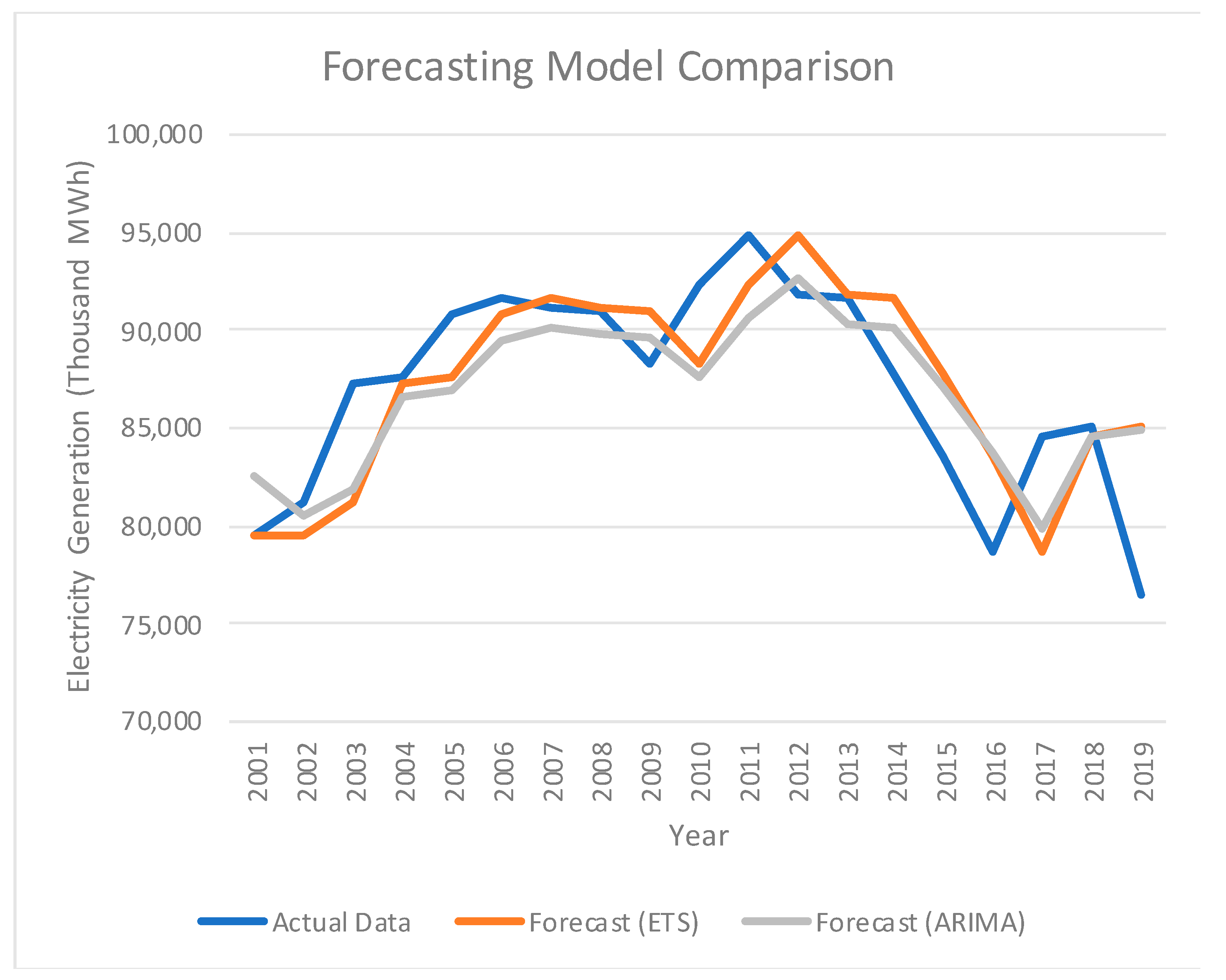
Using the Forecast Library in r, simple exponential smoothing and ARIMA models were fit to the annual state-level electricity generation dataset. The results of this procedure are presented graphically in Figure 2. Actual data is denoted in blue, simple exponential smoothing in orange, and ARIMA in grey. ETS stands for exponential triple smoothing of which simple exponential smoothing is a variant. It can be observed that the simple exponential smoothing forecast selects the most recent observation as the prediction for the current time step. The ARIMA model is governed by different equations, but ultimately yields similar results. However, superior performance is difficult to determine upon visual inspection alone.
AICc values for each of the models are presented in Table 3. A smaller value corresponds to a model that is better fit to the data. The ARIMA model slightly outperforms simple exponential smoothing for this dataset. Additional assessment is required before the optimal model can be determined.
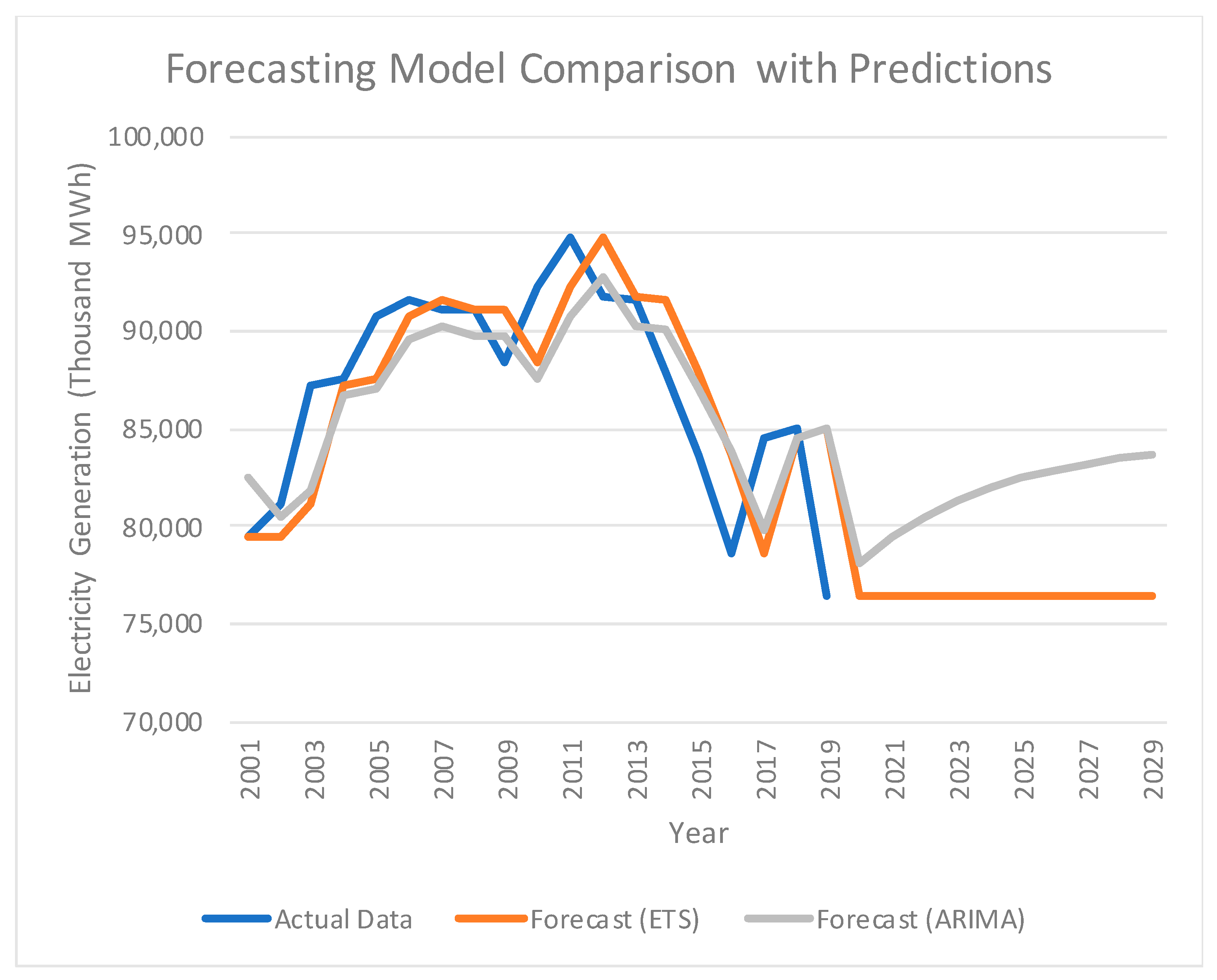
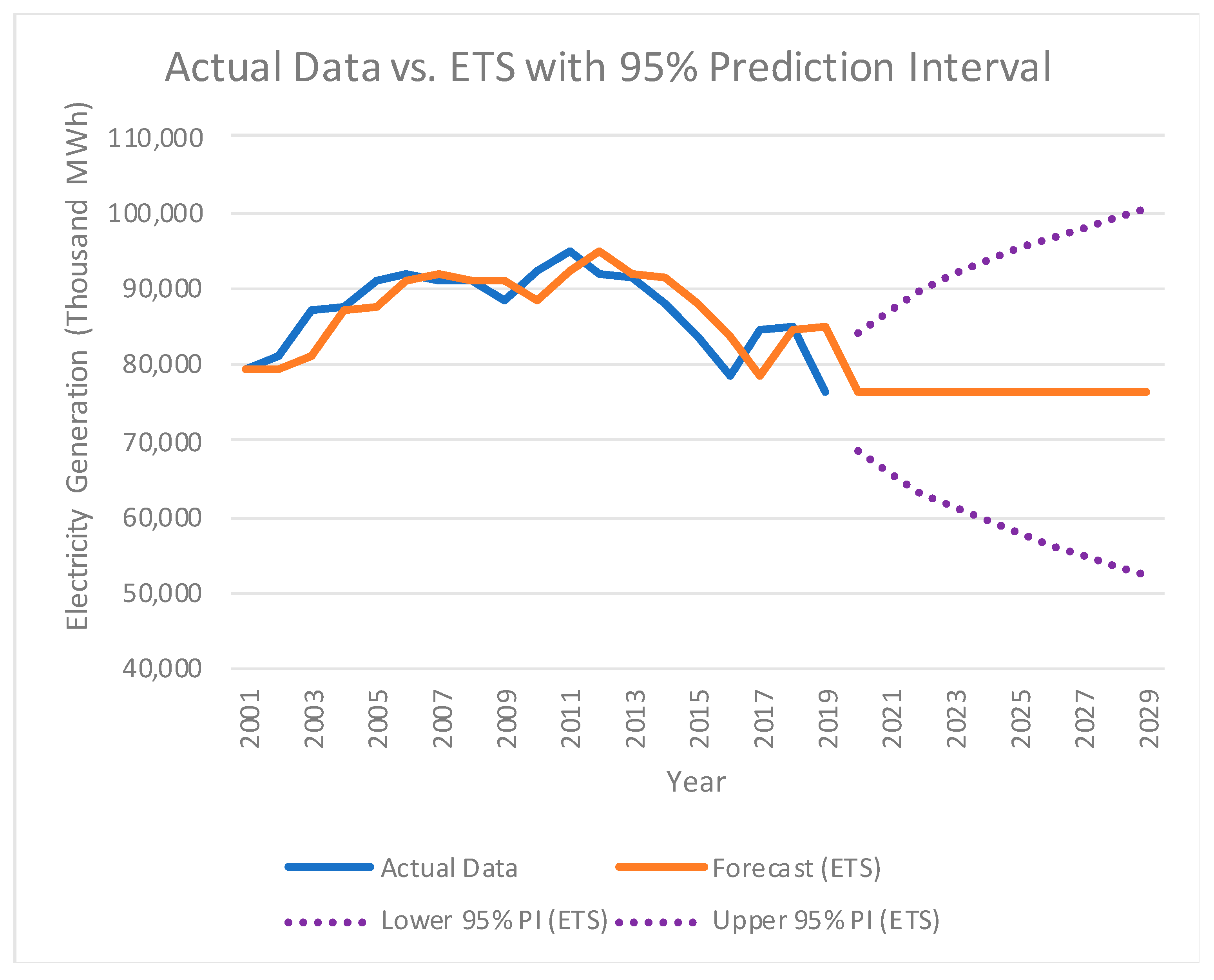
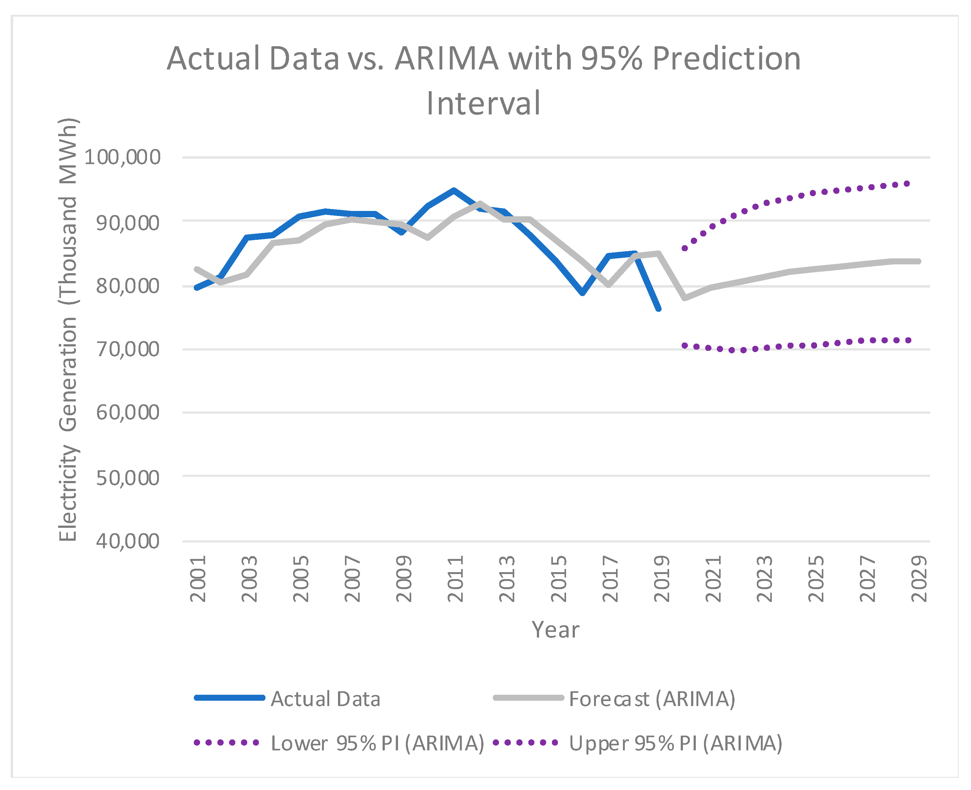
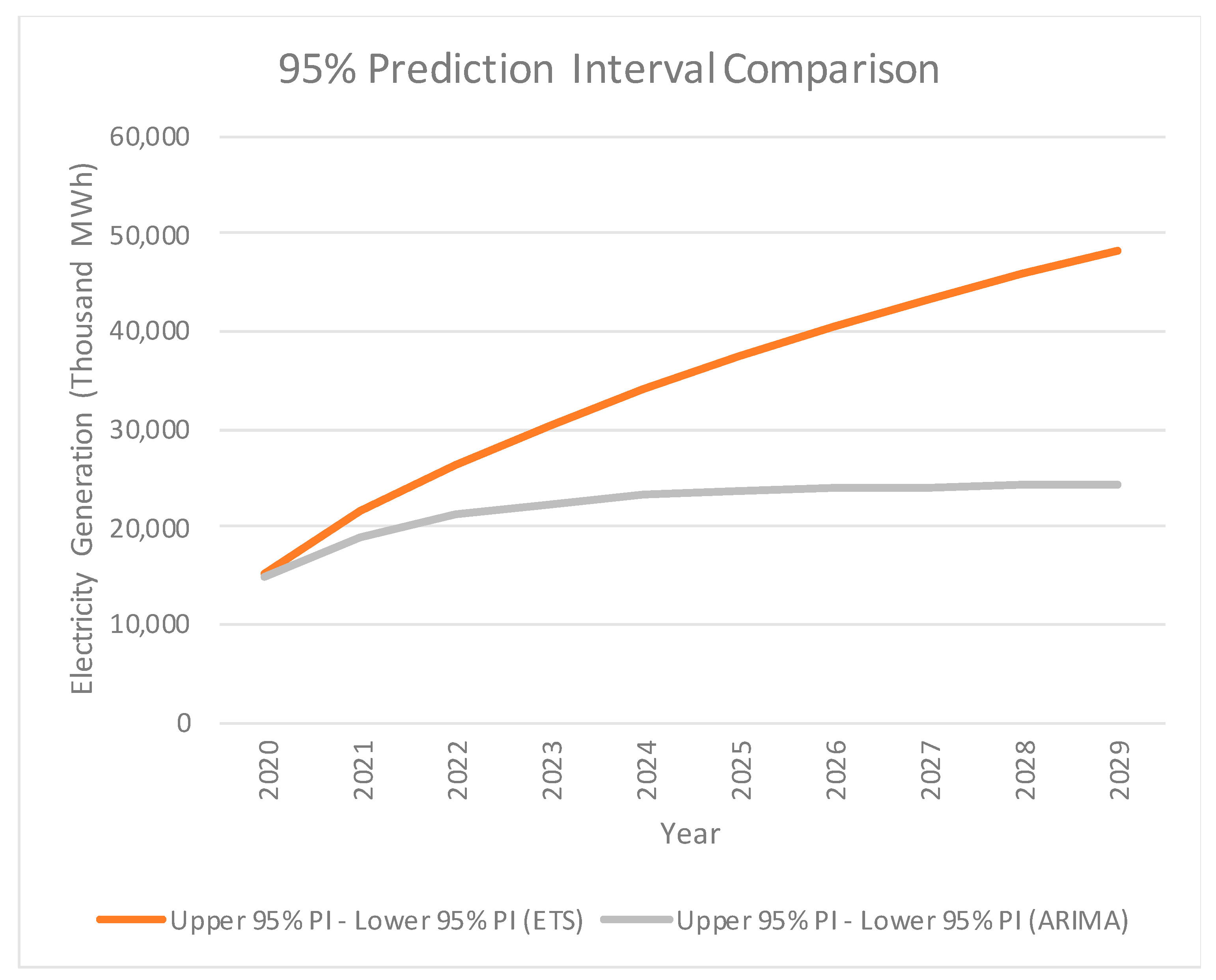
An alternative approach that augments visual inspection and summary statistical analysis is the evaluation of prediction intervals for each of the models. Figure 3 illustrates a 10-year prediction using each of the models. One shortcoming of simple exponential smoothing is that the prediction is given as a “flat” value. This behavior is unlikely to be representative of future energy generation scenarios. Alternatively, the ARIMA model trends upward before flattening out. Figure 4 and Figure 5 investigate the 95% prediction interval for simple exponential smoothing and ARIMA, respectively. In Figure 4, the prediction interval continuously expands as the forecast horizon increases. The prediction interval width at the final forecasted value is almost 50,000 (thousand MWh). Alternatively, ARIMA’s prediction interval provided in Figure 5 provides is greater than 24,000 (thousand MWh). This represents a significant reduction in uncertainty when compared to the simple exponential smoothing model.
To further demonstrate the difference between the two models, prediction interval width is plotted for the forecast horizon in Figure 6.
The ARIMA model is demonstrably superior when compared to the simple exponential smoothing model in terms of reduction in uncertainty. This observation coupled with the marginally better AICc value and non-flattening prediction behavior justifies the selection of the ARIMA model as an input for the sustainability assessment presented in the next section.

3.2. Sustainability Assessment of Proposed Electricity Portfolio Transition

Fitting a time series model to volatile data is a complex task. This is demonstrated by the summary statistic performance of both models and the uncertainty present denoted by the prediction interval widths. Initial electricity source portfolio shares are provided in Table 4. Sustainability assessment results are given for both prediction intervals and model predictions in Table 5. The 10-year percentage change for each of the footprints is provided in a min–max format. This is due to the data being provided in range format. Minimum values correspond to best-case performance for each of the footprint categories. Alternatively, maximum values provide a worst-case scenario. The upper 95 percent prediction interval scenario reflects a substantive increase in electricity from 2020 to 2029. This increase in electricity generation offsets the sustainability improvements where only carbon footprint is reduced in both minimum and maximum cases. With the exception of water’s maximum case, each of the other footprints increases in this scenario. For the ARIMA prediction, carbon and water footprints decrease. Land and cost footprints increase significantly. This is due to the higher values reported for the renewable technologies. The best performance is achieved for the lower 95% prediction interval. As electricity generation is decreased, the sustainability improvement will be more pronounced. Similarly to the ARIMA prediction performance, carbon and water decrease while land and cost increase. However, each of the footprints is decreased considerably from the model’s prediction. This finding suggests that the best sustainability performance will be achieved in the event that electricity generation decreases and a transition to renewable alternatives is conducted in a timely manner.
The results presented in Table 5 correspond to the scenario where coal is replaced in equal measure by solar and wind. It is beneficial to investigate the outcomes of alternative fulfillment strategies in the context of sustainability assessment. A comparison is provided in the next section.

3.3. Comparison of Different Fulfillment Strategies

Table 6 provides sustainability assessment results for the model prediction using different fulfillment strategies. Gamma is the variable that determines the behavior of the feedback loop used in the transition model. The solar-only scenario is denoted by gamma being equal to one. Alternatively, gamma equals zero for the wind-only strategy. Sustainability performance is provided in 0.2 increments for gamma. The broader implications of the results presented here are discussed in the next section.

4. Discussion

Two time series prediction methods, ARIMA and exponential smoothing, were used to develop a prediction of Missouri’s annual electricity generation. ARIMA exhibited superior performance measured across key summary statistics. Given these findings, a 10-year prediction of electricity generation was generated. The result of this procedure was used as an input for the sustainability assessment model.
Initial portfolio share values for coal, solar, and wind were determined and used for model initialization. Coal’s initial share (72.82%) was decreased at a rate of one-percent per year. Therefore, at the end of the simulation coal accounted for ten percent less of the portfolio. Solar (0.52%) and wind (3.76%) accounted for this decrease in portfolio share in equal measure. A ten-percent decrease in coal’s portfolio share resulted in a carbon footprint decrease (−6.12, −5.48) and water footprint decrease (−4.31, −5.77). Alternatively, land footprint increased (89.17, 36.44) and levelized cost increased (19.24, 25.07). Note that change in footprint is presented as a range of percentages instead of a discrete value. This is due to the literature reporting the values as a range derived from longitudinal studies. As reported in Table 1, some energy sources possess a larger range of values for a given indicator. Table 5 was generated to demonstrate the proposed transition’s sensitivity to both the range of sustainability values used and the uncertainty inherent in the model prediction.
With the exception of water footprint, each of the energy sources exhibit a range of values for each of the energy sources considered. Coal possesses a larger carbon and water footprint. However, coal has the smallest land footprint and a comparably low cost footprint. The magnitude of these differences are best understood in the context of scenarios presented in Table 5. The upper prediction interval demonstrated marginal improvement in carbon and water footprints and large increases to both land and cost footprints. This can be attributed to the increase in generation required not effectively offsetting coal’s decreased portfolio share. It can be observed that as electricity generation decreased, sustainability outcomes improved. As less energy is generated, the gains from decreasing coal’s portfolio share will be more pronounced. Less electricity is generated in this case and more of it is being fulfilled by renewable sources. Therefore, the lowest prediction interval returns the best sustainability performance.
For this research, an equal share of newly available portfolio was allocated to both wind and solar. Table 6 provides simulation results for different fulfillment strategies using the model prediction. The wind-only strategy achieves the best results for carbon, water, and cost footprints. Land footprint, however, is much larger and represents the worst performance. Alternatively, solar outperforms wind in land footprint performance alone. Intermediate gamma values demonstrate that sustainability performance improves as gamma is decreased. However, an optimal gamma value is not presented here as it is subject to derivation of a weighting scheme for each of the indicators consistent with stakeholder input.
The sustainability assessment results presented here underscore a few key considerations for energy decision makers tasked with transitioning current fulfillment strategies. First, a transition to existing renewable energy alternatives is not a panacea for climate change mitigation. Where renewables demonstrate positive performance in carbon and water footprint results, they perform negatively for land and cost. This is important to capture as sustainability involves more than just the relationship between carbon emissions and cost. Second, the impact of the sustainability performance presented here is not confined to the state of Missouri. Energy supply systems for both fossil fuel and renewable sources are national, and in some cases, global. Therefore, local energy decision making has global consequences. Lastly, the lower ninety-five percent prediction interval exhibited the best sustainability performance. This finding demonstrates the effectiveness of a strategy that couples a transition to renewables and improvements in technological efficiency that reduce electricity generation.
These findings are subject to some limitations that provide ample room for future research. The time series model predicts upward trending behavior that eventually flattens. Future values are unlikely to exhibit this behavior given the volatility of the historical data. Exploration of other prediction methods and use of higher resolution temporal data might generate more accurate and dependable results. Selection of an optimal gamma value should be determined with input from key stakeholders. This can be accomplished through the implementation of a Delphi Method and subsequent analysis. A similar stakeholder engagement procedure could also be followed to determine which scenario presented in Table 6 is chosen. If either of the upper intervals are used, then the outcome could be an increase in the net export of electricity or idle capacity installed. Alternatively, if the lower intervals are used then importing electricity might be required. The sustainability assessment model can be converted into a system dynamics model by incorporating additional feedback loops. At present, the rate of change constitutes the only feedback mechanism in the model. Candidate feedback loops include different policy effects, relationships between sustainability indicators, and response to system disruptions, among others. Further, the holistic sustainability approach could be extended to account for other metrics such as dispatchability, resilience, and job creation. The range of footprint values can be further specified by deploying state-specific data gathering efforts. If accomplished, the variability of findings would be decreased resulting in an improved model. Additionally, evaluation of other renewable energy technologies including distributed energy resources should be conducted. This would include the analysis of alternative energy mix scenarios subject to data availability. Solar and wind power were selected here given their comparably large share of Missouri’s renewable electricity portfolio. Lastly, an optimal implementation plan should be provided given a proposed energy transition. In the following section, a summary of the research is provided with concluding remarks.

5. Conclusions

Global energy portfolios are dependent on fossil fuel resources. This dependence results in the continuous emission of greenhouse gases that harm the environment. Beyond these concerns, energy sources also have an impact on other natural resources such as land and water. Therefore, energy decision makers must transition current portfolios to renewable alternatives while monitoring unintended sustainability impacts. The model presented provides a univariate time series prediction of annual electricity generation using publicly available data. The method exhibiting the best performance, ARIMA, was then used as an input for the sustainability assessment model that monitors the performance of a proposed transition using a footprint approach. Using Missouri as a testbed, coal’s share of the portfolio was decreased by one-percent annually and replaced with an equal share of wind and solar power over a ten-year period. Model findings demonstrate that such a transition would decrease carbon and water footprints while increasing land and cost footprints. However, the prediction intervals underscore the range of sustainability outcomes. The best performance occurs in the event that annual electricity generation decreases. This finding affects several aspects of management and governance.
Energy decision makers can change fulfillment strategies, but not antecedent demand behavior. Electricity and, more broadly, energy serve a crucial role in industrial processes. Therefore, sustainability performance similar to the approach provided here should guide product design and supply chain configuration. Practitioners can use these results to prioritize the sustainable procurement of raw materials through to more preferred end-of-life management techniques such as reuse [41]. Additionally, research and development efforts should design product architectures with improved efficiency. Governments can encourage such behavior through policy incentivization. Subsequently, energy use, and thus demand for electricity generation would decrease resulting in improved sustainability performance. Various decision makers are engaged in energy transitions and sustainability improvements. Policy professionals are tasked with passing laws that encourage the adoption of renewable energy technologies. Business entities should bring products to market that perform well on sustainability measures beyond profit. Lastly, energy decision makers must rapidly transition energy portfolios to renewable alternatives to limit further harm to the environment. The results presented here provide decision makers with a quantitative guide to evaluate the sustainability of proposed energy transition strategies more thoroughly.

Author Contributions

Conceptualization, J.H. and S.L.; methodology, J.H.; software, J.H.; validation, J.H.; formal analysis, J.H.; investigation, J.H. and S.L.; resources, J.H.; data curation, J.H.; writing—original draft preparation, J.H.; writing—review and editing, S.L.; visualization, J.H.; supervision, S.L.; project administration, S.L.; funding acquisition, S.L. All authors have read and agreed to the published version of the manuscript.

Funding

The authors gratefully acknowledge the DOE SUNSHOT GEARED program for partially funding this research through DOE Project DE-EE0006341.

Institutional Review Board Statement

Not applicable.

Informed Consent Statement

Not applicable.

Data Availability Statement

Annual electricity generation data is publicly available. This data can be accessed at [34]. Sustainability values used in this study are available in this article. Original values can be accessed at [32].

Conflicts of Interest

The authors declare no conflict of interest.

References

  1. International Energy Agency. Total Primary Energy Supply (TPES) by Source, World 1990–2017. Available online: https://www.iea.org/data-and-statistics?country=WORLD&fuel=Energy%20supply&indicator=Total%20primary%20energy%20supply%20(TPES)%20by%20source (accessed on 1 August 2020).
  2. International Energy Agency. CO2 Emissions by Energy Source, World 1990–2017. Available online: https://www.iea.org/data-and-statistics?country=WORLD&fuel=CO2%20emissions&indicator=CO2%20emissions%20by%20energy%20source (accessed on 1 August 2020).
  3. National Aeronautics and Space Administration. The Effects of Climate Change. Available online: https://climate.nasa.gov/effects/ (accessed on 1 June 2020).
  4. Singh, H.V.; Bocca, R.; Gomez, P.; Dahlke, S.; Bazilian, M. The energy transitions index: An analytic framework for understanding the evolving global energy system. Energy Strategy Rev. 2019, 26, 100382. [Google Scholar] [CrossRef]
  5. Meadowcroft, J. What about the politics? Sustainable development, transition management, and long term energy transitions. Policy Sci. 2009, 42, 323–340. [Google Scholar] [CrossRef]
  6. Verbong, G.; Geels, F. The ongoing energy transition: Lessons from a socio-technical, multi-level analysis of the Dutch electricity system (1960–2004). Energy Policy 2007, 35, 1025–1037. [Google Scholar] [CrossRef]
  7. Kern, F.; Smith, A. Restructuring energy systems for sustainability? Energy transition policy in the Netherlands. Energy Policy 2008, 36, 4093–4103. [Google Scholar] [CrossRef]
  8. Rutherford, J.; Coutard, O. Urban Energy Transitions: Places, Processes and Politics of Socio-technical Change. Urban Stud. 2014, 51, 1353–1377. [Google Scholar] [CrossRef]
  9. Tagliapietra, S.; Zachmann, G.; Edenhofer, O.; Glachant, J.M.; Linares, P.; Loeschel, A. The European union energy transition: Key priorities for the next five years. Energy Policy 2019, 132, 950–954. [Google Scholar] [CrossRef] [Green Version]
  10. Hölsgens, R.; Lübke, S.; Hasselkuß, M. Social innovations in the German energy transition: An attempt to use the heuristics of the multi-level perspective of transitions to analyze the diffusion process of social innovations. Energy Sustain. Soc. 2018, 8. [Google Scholar] [CrossRef]
  11. Schilling, T.; Wyss, R.; Binder, C.R. The resilience of sustainability transitions. Sustainability 2018, 10, 4593. [Google Scholar] [CrossRef] [Green Version]
  12. Busch, H.; McCormick, K. Local power: Exploring the motivations of mayors and key success factors for local municipalities to go 100% renewable energy. Energy Sustain. Soc. 2014, 4, 5. [Google Scholar] [CrossRef]
  13. Cowell, R. Sub-national government and pathways to sustainable energy. Environ. Plan. C Politics Space 2017, 35, 1139–1155. [Google Scholar] [CrossRef] [Green Version]
  14. Parkins, J.; Beckley, T.; Comeau, L.; Stedman, R.; Rollins, C.; Kessler, A. Can Distrust Enhance Public Engagement? Insights from a National Survey on Energy Issues in Canada. Soc. Nat. Resour. 2017, 30, 934–948. [Google Scholar] [CrossRef]
  15. Sánchez-Durán, R.; Luque, J.; Barbancho, J. Long-term demand forecasting in a scenario of energy transition. Energies 2019, 12, 3095. [Google Scholar] [CrossRef] [Green Version]
  16. Boroojeni, K.G.; Amini, M.H.; Bahrami, S.; Iyengar, S.S.; Sarwat, A.I.; Karabasoglu, O. A novel multi-time-scale modeling for electric power demand forecasting: From short-term to medium-term horizon. Electr. Power Syst. Res. 2017, 142, 58–73. [Google Scholar] [CrossRef]
  17. Ryu, S.; Noh, J.; Kim, H. Deep neural network based demand side short term load forecasting. Energies 2017, 10, 3. [Google Scholar] [CrossRef]
  18. Croonenbroeck, C.; Ambach, D. A selection of time series models for short- to medium-term wind power forecasting. J. Wind Eng. Ind. Aerodyn. 2019, 136, 201–210. [Google Scholar] [CrossRef]
  19. Le, T.; Vo, M.T.; Vo, B.; Hwang, E.; Rho, S.; Baik, S.W. Improving Electric Energy Consumption Prediction Using CNN and Bi-LSTM. Appl. Sci. 2019, 9, 4237. [Google Scholar] [CrossRef] [Green Version]
  20. Bernardi, M.; Petrella, L. Multiple season cycles forecasting model: The Italian electricity demand. Stat. Methods Appl. 2015, 24, 671–695. [Google Scholar] [CrossRef]
  21. Pfenninger, S.; Staffell, I. Long-term patterns of European PV output using 30 years of validated hourly reanalysis and satellite data. Energy 2016, 114, 1251–1265. [Google Scholar] [CrossRef] [Green Version]
  22. Rahman, A.; Srikumar, V.; Smith, A.D. Predicting electricity consumption for commercial and residential buildings using deep recurrent neural networks. Appl. Energy 2018, 212, 372–385. [Google Scholar] [CrossRef]
  23. de Oliveira, E.M.; Cyrino Oliveira, F.L. Forecasting mid-long term electric energy consumption through bagging ARIMA and exponential smoothing methods. Energy 2018, 144, 776–788. [Google Scholar] [CrossRef]
  24. Amasyali, K.; El-Gohary, N.M. A review of data-driven building energy consumption prediction studies. Renew. Sustain. Energy Rev. 2018, 81, 1192–1205. [Google Scholar] [CrossRef]
  25. Hyndman, R.J.; Athanasopoulos, G. Forecasting: Principles and Practice, 2nd ed.; OTexts: Melbourne, Australia, 2018; Available online: OTexts.com/fpp2 (accessed on 7 June 2020).
  26. Alabdulwahab, A.; Abusorrah, A.; Zhang, X.; Shahidehpour, M. Coordination of Interdependent Natural Gas and Electricity Infrastructures for Firming the Variability of Wind Energy in Stochastic Day-Ahead Scheduling. IEEE Trans. Sustain. Energy 2015, 6, 606–615. [Google Scholar] [CrossRef]
  27. Yang, Z.; Ce, L.; Lian, L. Electricity price forecasting by a hybrid model, combining wavelet transform, ARMA and kernel-based extreme learning machine methods. Appl. Energy 2017, 190, 291–305. [Google Scholar] [CrossRef]
  28. Amini, M.H.; Kargarian, A.; Karabasoglu, O. ARIMA-based decoupled time series forecasting of electric vehicle charging demand for stochastic power system operation. Electr. Power Syst. Res. 2016, 140, 378–390. [Google Scholar] [CrossRef]
  29. Gupta, R.A.; Gupta, N.K. A robust optimization based approach for microgrid operation in deregulated environment. Energy Convers. Manag. 2015, 93, 121–131. [Google Scholar] [CrossRef]
  30. Gude, V.; Corns, S.; Long, S. Flood Prediction and Uncertainty Estimation Using Deep Learning. Water 2020, 12, 884. [Google Scholar] [CrossRef] [Green Version]
  31. Weldu, Y.W.; Assefa, G. The search for most cost-effective way of achieving environmental sustainability status in electricity generation: Environmental life cycle cost analysis of energy scenarios. J. Clean. Prod. 2017, 142, 2296–2304. [Google Scholar] [CrossRef]
  32. Hadian, S.; Madani, K. A system of systems approach to energy sustainability assessment: Are all renewables really green? Ecol. Indic. 2015, 52, 194–206. [Google Scholar] [CrossRef]
  33. Shue, H. Responsible for what? Carbon producer CO2 contributions and the energy transition. Clim. Chang. 2017, 144, 591–596. [Google Scholar] [CrossRef] [Green Version]
  34. Energy Information Administration. Electricity Data Browser, Net Generation for All Sectors, Annual (Missouri). Available online: https://www.eia.gov/electricity/data/browser/#/topic/0?agg=2,0,1&fuel=vtvv&geo=000002&sec=g&linechart=ELEC.GEN.ALL-MO-99.A&columnchart=ELEC.GEN.ALL-MO-99.A&map=ELEC.GEN.ALL-MO-99.A&freq=A&ctype=linechart&ltype=pin&rtype=s&pin=&rse=0&maptype=0 (accessed on 16 June 2020).
  35. Prema, V.; Uma Rao, K. Development of statistical time series models for solar power prediction. Renew. Energy 2015, 83, 100–109. [Google Scholar] [CrossRef]
  36. Ferbar Tratar, L.; Strmčnik, E. The comparison of Holt-Winters method and Multiple regression method: A case study. Energy 2016, 109, 266–276. [Google Scholar] [CrossRef]
  37. Yuan, C.; Liu, S.; Fang, Z. Comparison of China’s primary energy consumption forecasting by using ARIMA (the autoregressive integrated moving average) model and GM(1,1) model. Energy 2016, 100, 384–390. [Google Scholar] [CrossRef]
  38. Sen, P.; Roy, M.; Pal, P. Application of ARIMA for forecasting energy consumption and GHG emission: A case study of an Indian pig iron manufacturing organization. Energy 2016, 116, 1031–1038. [Google Scholar] [CrossRef]
  39. Hyndman, R.; Athanasopoulos, G.; Bergmeir, C.; Caceres, G.; Chhay, L.; O’Hara-Wild, M.; Petropoulos, F.; Razbash, S.; Wang, E.; Yasmeen, F. Forecast: Forecasting Functions for Time Series and Linear Models. R Package Version 8.12. 2020. Available online: http://pkg.robjhyndman.com/forecast (accessed on 15 August 2020).
  40. Hyndman, R.J.; Khandakar, Y. Automatic time series forecasting: The forecast package for R. J. Stat. Softw. 2008, 26, 1–22. [Google Scholar]
  41. Environmental Protection Agency, Climate Change and the Life Cycle of Stuff. Available online: https://19january2017snapshot.epa.gov/climatechange/climate-change-and-life-cycle-stuff_.html (accessed on 15 August 2020).
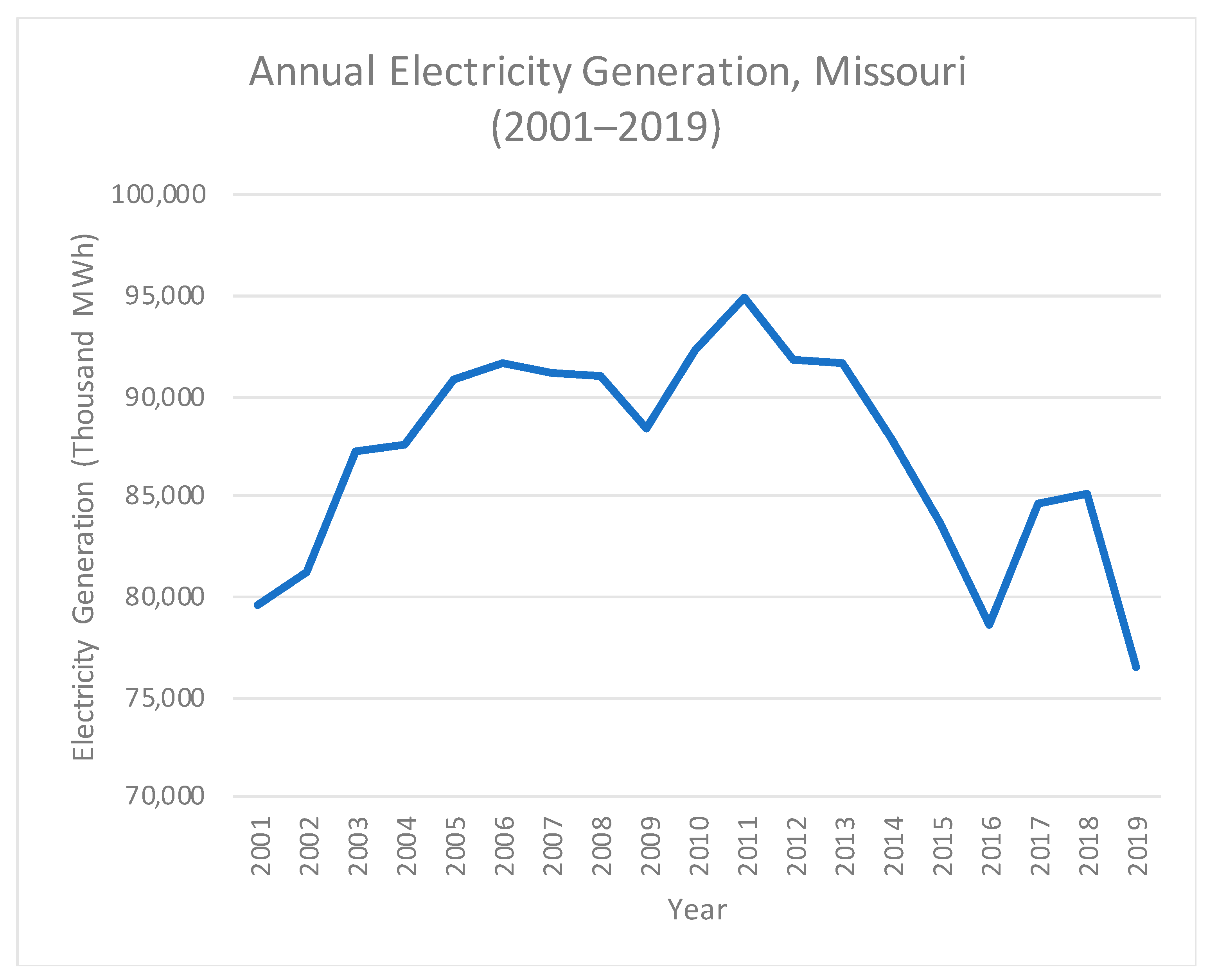
Figure 1. Total Electricity Generation, Missouri 2001–2019.
Energies 14 00141 g001
Figure 2. Forecasting Model Comparison.
Energies 14 00141 g002
Figure 3. Forecasting Model Comparison with Predictions.
Energies 14 00141 g003
Figure 4. Actual Data vs. exponential triple smoothing (ETS) with 95% Prediction Interval.
Energies 14 00141 g004
Figure 5. Actual Data vs. ARIMA with 95% Prediction Interval.
Energies 14 00141 g005
Figure 6. 95% Prediction Interval Width Comparison.
Energies 14 00141 g006
Table 1. Sustainability Indicators of Various Energy Types.
Energy TypeCarbon Footprint (g CO2/kWh)Water Footprint (m3/kWh)Land Footprint (m2/kWh)Cost (Cents/kWh)
Coal8.34 × 102–1.03 × 1035.40 × 10−4–2.09 × 10−38.30 × 10−5–5.67 × 10−43.77–5.85
Wind: onshore6.90–1.45 × 1013.60 × 10−62.17 × 10⁻³–2.64 × 10−34.16–5.72
Solar Photovoltaic1.25 × 101–1.04 × 1021.51 × 10−47.04 × 10⁻⁴–1.76 × 10−31.09 × 101–2.34 × 101
Table 3. Corrected Akaike Information Criterion (AICc) for Time Series Prediction Models.
ModelAICc
ETS (A,N,N)375.56
ARIMA (1,0,0)373.64
Table 4. Initial Model Configuration.
Electricity SourceInitial Portfolio Share (Xi)
Coal72.82%
Wind3.76%
Solar0.52%
Table 5. Sustainability Assessment Results.
Footprint Simulation Results
10-Year % Change (Min, Max)CarbonWaterLandCost
Upper 95% PI(−1.83, −1.16)(0.07, −1.46)(97.82, 42.68)(24.70, 30.79)
Model(−6.12, −5.48)(−4.31, −5.77)(89.17, 36.44)(19.24, 25.07)
Lower 95% PI(−11.32, −10.71)(−9.61, −10.99)(78.69, 28.88)(12.64, 18.15)
Table 6. Sustainability Evaluation for Different Fulfillment Strategies.
Carbon FootprintWater FootprintLand FootprintCost Footprint
γ MinMaxMinMaxMinMaxMinMax
1
(solar-only)
−6.07%−4.89%−2.46%−5.29%46.61%28.72%29.84%42.60%
0.8−6.09%−5.12%−3.20%−5.48%64.11%31.82%25.63%35.67%
0.6−6.11%−5.36%−3.94%−5.68%80.97%34.90%21.38%28.63%
0.5−6.12%−5.48%−4.31%−5.77%89.17%36.44%19.24%25.07%
0.4−6.13%−5.60%−4.68%−5.87%97.21%37.97%17.10%21.49%
0.2−6.15%−5.84%−5.42%−6.06%112.87%41.01%12.77%14.24%
0
(wind-only)
−6.16%−6.07%−6.16%−6.25%127.98%44.03%8.41%6.87%
Publisher’s Note: MDPI stays neutral with regard to jurisdictional claims in published maps and institutional affiliations.