3D Electromagnetic Field Analysis Applied to Evaluate the Accuracy of a Voltage Transformer under Distorted Voltage

Abstract

Voltage transformers (VTs) are an important element of the measuring system that allows measuring the energy flow in medium and high voltage networks. Additional problems with the accuracy of the measurement introduced by the appearance of sources and nonlinear receivers cause deformation of the voltage shape in the energy system. Due to the high metrological requirements, the design of voltage transformers requires high accuracy (for class 0.2 ΔU ≤ 0.2, phase displacement ≤10 min), which is not possible with the use of analytical methods using approximate models. Therefore, only the application of numerical modeling by the finite element method, taking into account real three-dimensional phenomena, allows achieving high modeling accuracy. The article concerns the phenomenon of the influence of voltage higher harmonics of supply voltage on the accuracy (up to the 100th harmonic) of the measuring inductive voltage transformer (IVT). The applied modeling method takes into account the phenomena in the transformer core and the circuit equations resulting from the winding arrangement, which allows for the study of the deformation voltage transformation. Experimental tests on a real model to evaluate the method used were necessary. The article presents simulations for a model transformer, and results have been confirmed by experimental tests.

1. Introduction

Maintaining appropriate voltage quality in distribution networks is gaining importance, because of application of nonlinear receivers and distributed generation units with uneven electric power production depending on external factors [1]. A special case of distributed generation are renewable energy generating units with electric power up to 40 kW and 200 kW, which are connected to the distribution network. Among them, the most popular technologies are photovoltaic panels and small wind farms. One of their characteristic features is grid connection through an inverter. Modulation methods of shaping the output voltage of voltage inverters cause significant deformation of the output signals. Harmonics of the supply voltage are caused also by network users’ nonlinear loads connected to all voltage levels of the supply system [2].

There is a problem with the accuracy of measuring the power at transmission and distribution substations [3,4]. A measuring voltage transformer (VT) is a component of the power measuring system; it is a device that transforms signals but adds its own transformation errors to the measured values. The International Electrotechnical Commission (IEC) standards [5,6] oblige designers to determine and limit these errors. If the instantaneous values of the voltage supplied to the VT are too high, its core becomes saturated. This changes the parameters of the equivalent circuit, such as leakage reactance, as well as magnetization reactance and resistance, representing the losses in the core and, thus, the values of the instantaneous secondary voltages. Therefore, an analysis of the behavior of the inductive VT supplied with distorted voltage was performed to determine the transformation accuracy of the distorted voltage by the VT.

The 3D finite element method was previously used by the authors in the design of electromagnetic devices such as motors [7], power transformers [8], instrument transformers [9], and other types of converters. It was used both in the design of magnetic circuits [10] and insulation [11,12], as so in steady states as in transient, when supplied with direct and sinusoidal current.

The research, which was carried out on the basis of very approximate analytical models [13,14], did not take into account most of the phenomena that are included in the three-dimensional calculations of the electromagnetic field. The use of 3D modeling to test the accuracy of VTs (voltage transformers) powered by distorted voltages is an aspect that has not yet been addressed in the literature. Experimental tests on a real model to evaluate the method used were necessary.

Measurement methods and systems for determining the transformation errors of current and voltage transformers based on various principles are described in the literature [15,16,17].

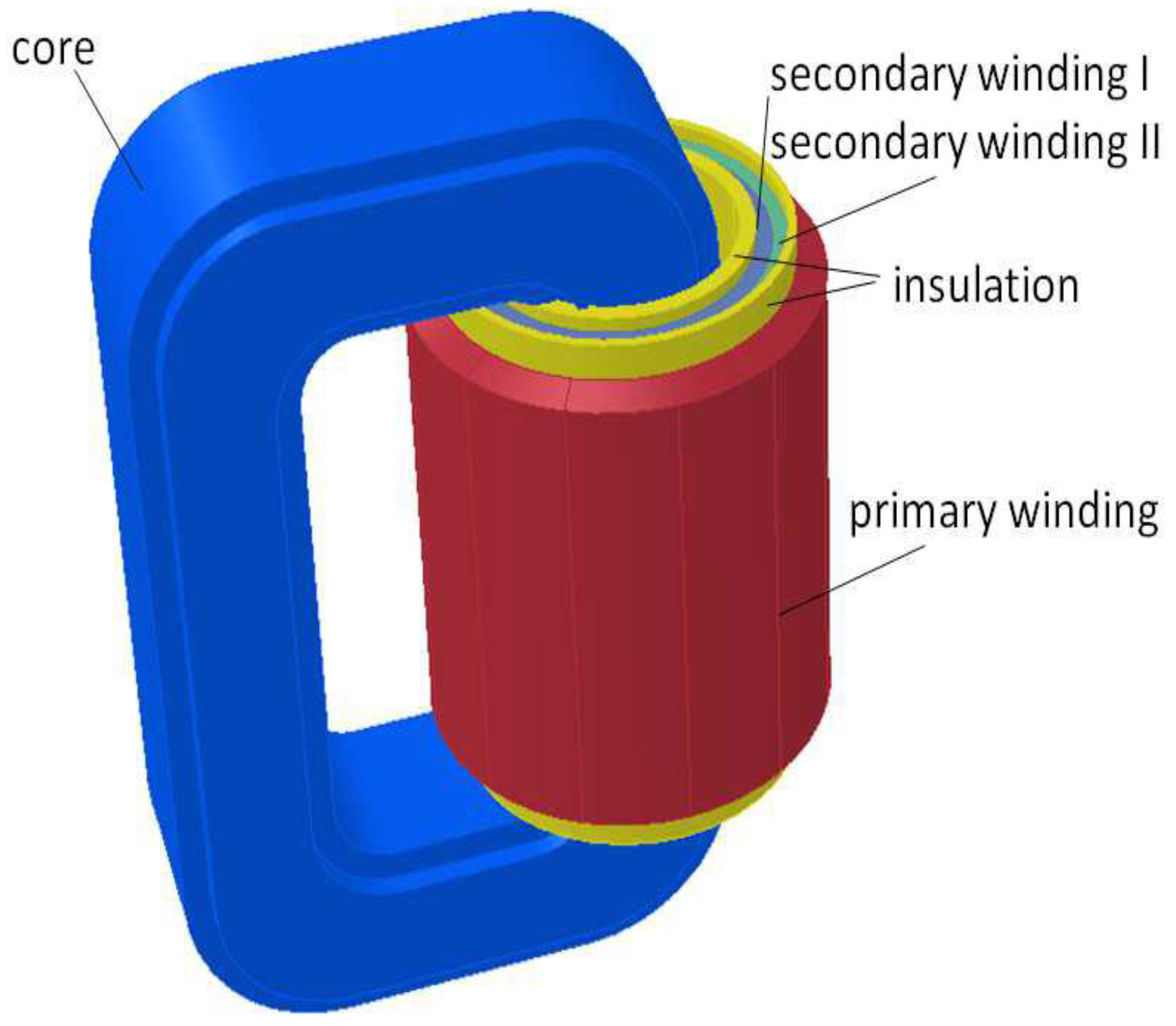
2. Construction of VT

The analysis of the measurement operation of the medium voltage (MV) voltage transformer was carried out for the 2000 V/100 V VT. The magnetic core of this VT is made from cold-rolled steel sheets and composed of two parts connected together in the middle of the windings. Figure 1 presents a 3D model of the tested measuring VT (2000 V/100 V).

Producers usually do not provide the initial properties of the magnetic materials in their catalogs. The parameters of magnetic cores of inductive voltage transformers defined by the magnetization curve and the active power losses have big influence on their transformation accuracy. The use of an inappropriate magnetization curve for computation leads to large discrepancies between the calculated and actual values of transformation errors. Therefore, the designers of VT should first measure the actual magnetic characteristics of the magnetic material used for the core [18,19,20].

The magnetization characteristics presented in Figure 2 were determined for the tested VT according to the equations:

$$B_m=\frac{1}{z_s{S}_{Fe}}{{\displaystyle \int }}^{ }{u}_{s}dt,H_m=\frac{i_p{z}_p}{l_{Fe}}$$

(1)

where i_p—the instantaneous value of the primary current,

u_s—the instantaneous value of the secondary voltage, z_p and z_s—are numbers of turns of the primary and the secondary windings, S_Fe—the surface area of the cross section of the magnetic core, and l_Fe—the average magnetic flux path in the core.

Figure 2 shows the measured magnetic properties of the magnetic core used in the tested VT.

Figure 3 shows the measuring system. The four channels of the oscilloscope enable measurements of the following voltages channels: CH1—the primary voltage of tested VT through the high voltage probe HVP, CH2—the voltage proportional to the primary current from the current shunt (CS) whose resistance is equal to 100 Ω, CH3—the voltage from first secondary winding of tested VT, and CH4—the voltage from second secondary winding of tested VT. The oscilloscope enables to find the integral of the secondary voltage waveform.

During the tests, the magnetization characteristics of the core up to 1.2 T were determined for the safety of people and devices. To extend the curve to the value of saturation induction, Froelich’s method was used [20], as it has been validated to yield excellent results.

3. Mathematical Model of VT

The analysis was performed using the 3D field-circuit method by coupling Maxwell’s equations in the area of the tested object with the equation for circuit outside the area (the load connected to the terminals of the modeled device) [7,10,21]. This enables to calculate the currents and voltages induced in the secondary circuit. This method uses the equation of the Helmholtz type for the harmonic electromagnetic field, and it is the most direct method of determining the characteristics of the current error and the phase displacement of instrument transformers [22,23].

For steady-state condition of a VT, the electromagnetic field can be treated as harmonic, therefore complex magnetic vector potential A (B = ∇ × A) may be used. Using quasi-static of Maxwell’s equations leads to an equation of complex time-harmonic Helmholtz type equation.

$${\nabla }^2\underset{\_}{\mathit{A}}-\mu \nabla \left(\frac{1}{\mu }\right)\times \nabla \times \underset{\_}{\mathit{A}}-j\omega \mu \sigma \underset{\_}{\mathit{A}}=-\mu \underset{\_}{{\mathit{J}}_w}$$

(2)

$$\underset{\_}{\Psi }=\frac{n_s}{S_s}\underset{{\Omega }_s}{{\displaystyle \int }}\underset{\_}{\mathit{A}}·{\mathit{l}}_{s}dv$$

(3)

$${\underset{\_}{U}}_s=j\omega \underset{\_}{\Psi }=R{\underset{\_}{I}}_s$$

(4)

The boundary conditions for magnetic vector potential are A × n = 0 and V = 0 for electric scalar potential at the boundary of the entire system with the surrounding air. This boundary condition means that at the boundary appears only a tangential part of the magnetic flux density B vector where n is a normal vector to the surface boundary.

The combination of the field-circuit method and the 3D space-and-time analysis allows determining the operation of VTs during the supply of distorted voltage. The time-varying electromagnetic field is described by an equation of the diffusion type [24,25].

$$curl\left(\frac{1}{\mu } curl \mathit{A}\right)=\sigma \left(-\frac{\partial \mathit{A}}{\partial t}-gradV\right)$$

(5)

$$\Psi =\frac{n_s}{S_s}{{\displaystyle \int }}_{{\Omega }_s}\mathit{A}·{\mathit{l}}_{s}dv$$

(6)

$$u_s=\frac{d\Psi }{dt}=R{i}_s$$

(7)

where ω is angular frequency of voltage, μ is the permeability, σ is the conductivity of materials, and R is the load resistance of the voltage transformer. Ψ is the magnetic flux passing through the secondary coil where n_s and S_s are the number of turns and the cross-sectional area of the secondary coil, respectively, Ω_s is the volume of the secondary winding, and l_s is the unit tangential vector along the direction of the secondary current in the winding. The boundary conditions are $A\times n=0$ and V = 0 at the boundary of the whole system with the surrounding air.

The secondary voltage is determined and compared with the same secondary voltage of load circuit Equations (3) and (4) or (6) and (7).

Both these methods were used, and the nonlinear magnetic characteristics of the ferromagnetic material B-H curve were considered. As in previous research [10,22,23,24,25], a method was taken into account for power losses in laminated cores [19].

The commercial software OPERA 3D was used to compute field distributions. For steady state, the ELEKTRA STEADY-STATE module was used, and for the 3D space-and-time analysis module, ELEKTRA TRANSIENT.

The mesh of 2,072,724 elements for a quarter of the 3D model (with using symmetry of system) was the result of an accuracy analysis. Further mesh refinements did not change the solution and improve accuracy. The time step of 5.00 × 10⁻⁰⁵ s was used for the space-and-time analysis. Figure 4 shows the method of measuring VT transformation errors at different voltage harmonics.

Voltage errors of the tested VT during transformation of distorted voltage’s higher harmonics were determined using the measuring system, as given in detail in [5,26] (Figure 4).

Measured quantities:

• The RMS values of a given higher harmonic in the input voltage of TVT: U_TVThk.
• The RMS values of a given higher harmonic in the output voltage of DA: U_DAhk.
• The phase shift of a given harmonic in the output voltage of DA in relation to the same frequency harmonic in the input voltage of TVT: φ_TVTDA.

A wideband voltage divider was used as the source of the reference voltage [27]. The calibration method for this divider is presented in [28,29]. The output voltage of the divider and the secondary voltage of the tested VT were simultaneously measured by two voltage channels of the digital power meter. Implemented in this device, the fast Fourier transform algorithm enables determination of up to 100th harmonics. Additionally, usage of the differential high impedance wideband converter provided measurements of the differential voltage between the high potential terminal of the tested VT’s secondary winding and the high potential terminal of the output of the reference voltage divider. This enabled to determine the voltage composite error of the tested VT for verification of the highest possible value of the measured voltage error. A power amplifier controlled by an arbitrary waveform generator was used to supply the step-up voltage to the VT. This enables the generation of distorted primary voltage with an effective RMS value reaching 3 kV, assuming that RMS of the basic harmonic (50 Hz) is rated and the RMS of higher harmonic (up to 100th) has been set to 10% of this value.

The voltage ratio error of transformation of the distorted voltage’s k-order harmonic ΔU_kh, expressed in percent, is given by the formula:

$$\Delta U_{kh}=\frac{U_{TVTkh}-U_{RVDkh}}{U_{RVDkh}}·100\%$$

(8)

where U_TVTkh is the RMS value of the k-order harmonic of the distorted secondary voltage of the tested voltage transformer, and U_RVDkh is the RMS value of the k-order harmonic of voltage of the reference voltage divider.

The expended combined uncertainties of the composite measurements of the values of voltage and phase errors are calculated for the RMS value of the composite error equal to ±1.0% with the coverage factor equal to 2 to ensure the level of confidence of about 95% are equal to (voltage error/phase error) ±0.02%/±0.02° for 50 Hz and ±0.1%/±0.1° for 5 kHz. Calculation of the uncertainty of measurements of the values of phase and voltage errors at harmonics for transformation of distorted voltage is very complex, therefore it was not presented in detail in the proposed for publication paper. Measured quantities are: the RMS values of a given higher harmonic in the input voltage of the VT (measured thorough the RVD) and in the output voltage of the differential high impedance wideband converter as well as the phase shift of a given harmonic in the output voltage of the differential high impedance wideband converter in relation to the same frequency harmonic in the input voltage of the VT (measured thorough the reference voltage divider (RVD)). The accuracy of reference voltage divider is equal to ±0.1%/±0.1° for 50 Hz and ±1%/±1° for 5 kHz (explanation in Appendix A), the accuracy of the high impedance wideband converter of differential voltage to single ended voltage is equal to ±1%/±1° from 50 Hz to 5 kHz, and the accuracy of the digital power meter is equal to ±0.15%/±0.3 for 50 Hz and ±2%/±3° for 5 kHz.

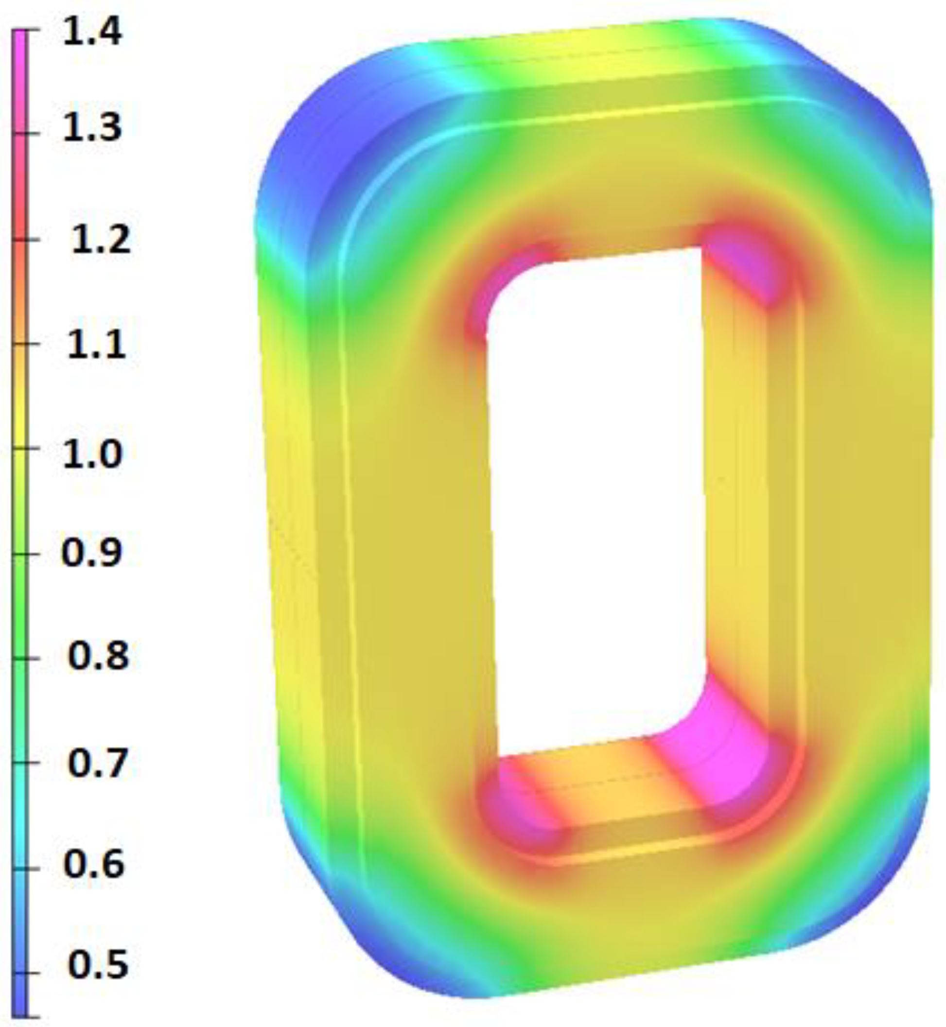
4. Results of Computations and Tests

Calculations and measurements of the real-world model were performed during the supply of distorted voltage to the VT, and their results were compared.

The starting point of the study was to determine the accuracy of the tested VT model for the transformation of sinusoidal voltage of frequency 50 Hz in accordance with the IEC standard. The electronic electricity meters currently used have very low power demand, often below 1 VA, at cosφ = 1. Therefore, a resistive load of 2 MΩ was used.

The IEC standard defines transformation errors as voltage error [6]:

$$\Delta U=\frac{U_s{K}_n-U_p}{U_p}·100\%$$

(9)

and phase displacement

$${\delta }_u={\phi }_{u_s}-{\phi }_{u_p}$$

(10)

Figure 4 shows the diagram of the measuring system used for assessing the accuracy of harmonic transformation of distorted voltages by VTs, and for verifying the accuracy of phase displacement measurement by a digital watt meter.

As a result of the analyses, the uncertainty of measurement of voltage errors and phase displasement of voltage transformers at different harmonics of the supply voltage was determined for this measurement system (

Table 1. Uncertainty of measurement of measuring system.

Uncertainty of Measurement	Voltage Errors	Phase Displacement
50 Hz	±0.02%	±0.02°
250 Hz	±0.05%	±0.05°

).

Figure 5 shows the distribution of the magnetic field in the transformer core, obtained as a result of field-circuit analysis at 50 Hz.

The results show that the values of voltage errors and phase displacement for the first harmonic (taking into account the measurement uncertainty of voltage errors and phase displacement) ranged from +0.13% to +0.17% and from −1 min to +3 min, respectively. This means that the measurement and calculation results are consistent (

Table 2. Comparison of calculated and measured voltage errors of the tested VT at rated 50 Hz sinusoidal voltage and load 2 MΩ.

Primary Voltage 100% UN	Secondary Winding I
	Measurement	Computation
Voltage errors [%]	0.15	0.15
Phase displacement [min]	0.9	2.4

).

The European Standard EN 50160 [30] recommends acceptable amplitude values for individual harmonics (Figure 6). Next, the VT was tested by supplying distorted voltages with the amplitudes above the values permitted by the EN standard.

The worst case was assumed as an example for the calculation. The fifth harmonic superimposed on the first one, which gives the highest instantaneous value of the primary voltage, was chosen as a calculation example (Figure 7). It was assumed that both harmonics (1 and 5) are not showing phase displacement toward each other, and the amplitude of the fifth harmonic is 10% and 40% of that of the first harmonic (6% allowed). In these cases, the total harmonic distortion (THD) is 0.1, 0.4, with 10% and 40% amplitude, where

$$THD=\frac{\sqrt{{\sum }_{k = 2}^n{U}_{rms}^2-U_1^2}}{U_1}$$

(11)

Abbreviation 1H means the first harmonic with amplitude of 100% of the rated value. 1H + 10% 5H means the overlay on the first harmonic (with amplitude of 100% of the rated value) of the fifth harmonic with an amplitude of 10% of the amplitude the first harmonic, etc.

The transformation errors should be calculated in a steady state. When supplying a VT system (which is the resistance-inductive system) with sinusoidal and distorted periodic voltage, a transient state appears and disappears after five time constants, which significantly extends the time of calculations. Hence, during calculations, according to the theory, the phase shift of voltages 1 and 5 of the harmonic was used by the angle φ_u = φ, where φ is the angle of equivalent impedance of the voltage transformer system, different for each harmonic. This avoided the transient state.

The RMS value of a varying periodically voltage is defined by the formula

$$U=\sqrt{\frac{1}{T}\underset{0}{\overset{T}{\int }}{u}^{2}dt}$$

(12)

Secondary voltages as a function of time were calculated by the field-circuit method.

In addition, discrete Fourier transform (DFT) was used to calculate the harmonic content of the calculated secondary voltage and their maximum values (Figure 8). These values were compared with the imposed harmonic amplitudes in the supply voltage and with the results of the measurements. The results of this analysis were consistent with the results of the measurements.

Based on this, voltages as a function of time were calculated in accordance with Formula (12), their RMS values, and then, on the basis of Equation (9), voltage errors, and phase displacement (10) at the passage of primary and secondary voltage through zero.

During the testing of the real-world model, it was assumed that the primary voltage contained the first harmonic with a frequency of 50 Hz, and one higher harmonic in the frequency range of 100 Hz to 5 kHz with an effective value of 10% of the main harmonic. The differences in the measured transformation errors at different phase shifts between the first and higher harmonic were also considered (

Table 3. Comparison of calculated and measured voltage errors of the tested VT at distorted voltage and load 2 MΩ.

Transformation Errors	Secondary Winding I
	Measurement	Computation
Primary voltage 100% UN
Voltage errors [%]	0.15	0.15
Phase displacement [min]	0.93	2.4
Primary voltage 100% UN+10%5H
Voltage errors [%]	0.15	0.14
Phase displacement [min]	−0.15	−0.69
Primary voltage 100% UN+40%5H
Voltage errors [%]	—	0.13
Phase displacement [min]	—	−0.14

).

Since the accuracy of the measurements is within the range for voltage errors from +0.13% to +0.17% and for the phase shift from −3 min to +3 min for the base harmonic 50 Hz, and for the fifth harmonic the range is larger (Table 1), it means that the results of measurements and calculations (Table 3) are similar.

It can be seen that the transformation error of the 2000 V/100 V voltage transformer does not exceed the limit specified for the accuracy class 0.2 for the supplied distorted voltage with the fifth harmonic with the amplitude of 10%, and even 40%, of that of the first harmonic.

The VT’s transformation accuracy of higher harmonics of distorted primary voltages was tested under the following conditions: the primary winding was supplied with the distorted primary voltage composed of the rated primary voltage and additional single higher harmonic, the secondary winding was loaded only with impedance resulting from connection to its secondary winding voltage channel of the digital power meter (2 MΩ).

The differences in the measured transformation errors at different phase shifts between the first and higher harmonic were also considered. Figure 9 shows the measured values of the voltage errors and phase displacements.

In Figure 9, one can observe that the results of testing of the separate voltage errors for the first (50 Hz (Table 2, Table 3 and

Table 4. Result of voltage errors and phase displacement of the tested VT at different voltage and load 2 MΩ.

Secondary Winding I	Voltage Errors [%]	Phase Displacement [min]
Primary voltage 100% UN	0.15	0.9
Primary voltage 10% 5H	0.18	−2.9
Primary voltage 100% UN+10% 5H	0.15	−0.15

)) and fifth harmonics (250 Hz (Table 4)) overlap with the results of the calculations.

An increase of the harmonic frequency causes a decrease of accuracy of transformation of VT, and for the 100th order harmonic, voltage error reaches about −0.6%, while phase displacement does not exceed 52 min.

It was observed that higher harmonics with the amplitude of 10% of the first harmonic amplitude, when transferred to the secondary voltage, have little effect on the errors in the resulting voltage curve (Table 4).

Moreover, errors in the transfer of individual harmonics can be significant, as they can affect the power of the receivers, because the active power is the sum of the active powers of the individual harmonics (Figure 9).

5. Conclusions

As a result of the research, it can be concluded that the transformation errors of MV voltage transformers do not cause significant errors in voltage measurements when supplied with distorted voltage (even assuming the worst case yielding the highest instantaneous value of the primary voltage, when the fifth harmonic with amplitude of 40% of the amplitude of the first harmonic was superimposed without delaying on the first harmonic). Value 40% (Figure 7) significantly exceeds the value of the fifth harmonic amplitude permitted by the standard and amounting to 5%.

According to the standard [5], under a high impedance load, the VT response for medium voltages is usually sufficient up to 2 kHz (40th), and also for lower frequencies.

Additionally, the shapes of the secondary voltages (transformed by VT) are consistent with the shapes of the primary voltages. The accuracy of the transformation, when supplied with distorted voltage, complies with the class of the voltage transformer (for class 0.2 ΔU ≤ 0.2, phase displacement ≤10 min). The results of calculations and measurements for the tested voltage transformer show that the voltage distortion does not cause significant measurement errors.

Physical tests require the construction of a prototype of a voltage transformer. Conformity of the results of calculations and tests confirms the possibility of using the field-circuit method to assess the accuracy of voltage transformers at the design, and also in the case of a non-sinusoidal supply already.

This study was conducted for a specific VT; however, in general, the quality of the transformation depends on the design and materials used. Therefore, it is profitable to apply field-circuit simulation before building a prototype. The presented methodology can be used, for any inductive voltage transformer, to determine the ability of the voltage transformer to map the distorted voltage, especially since this phenomenon appears more and more frequently in power grids.

The use of 3D modeling to test the accuracy of voltage transformers powered by distorted voltages is an aspect that has not yet been addressed in the literature. The research, which was carried out on the basis of very approximate analytical models, did not take into account most of the phenomena that are included in the three-dimensional calculations of the electromagnetic field.

References

1. Xu, W.; Liu, Y. A method for determining customer and utility harmonic contributions at the point of common coupling. IEEE Trans. Power Deliv. 2000, 15, 804–811. [Google Scholar] [CrossRef] [Green Version]
2. Bajaj, M.; Singh, A.K.; Alowaidi, M.; Sharma, N.K.; Sharma, S.K.; Mishra, S. Power Quality Assessment of Distorted Distribution Networks Incorporating Renewable Distributed Generation Systems Based on the Analytic Hierarchy Process. IEEE Access 2020, 8, 145713–145737. [Google Scholar] [CrossRef]
3. Filipović-Grčić, D.; Filipović-Grčić, B.; Krajtner, D. Frequency response and harmonic distortion testing of inductive voltage transformer used for power quality measurements. Procedia Eng. 2017, 202, 159–167. [Google Scholar] [CrossRef]
4. Chen, Y.; Huang, Z.; Duan, Z.; Fu, P.; Zhou, G.; Luo, L. A Four-Winding Inductive Filtering Transformer to Enhance Power Quality in a High-Voltage Distribution Network Supplying Nonlinear Loads. Energies 2019, 12, 2021. [Google Scholar] [CrossRef] [Green Version]
5. IEC\TR 61869-103. Instrument Transformers—The Use of Instrument Transformers for Power Quality Measurement; International Electrotechnical Commission: Geneva, Switzerland, 2012. [Google Scholar]
6. IEC 61869-3. Instrument Transformers—Part 3: Additional Requirements for Inductive Voltage Transformers; International Electrotechnical Commission: Geneva, Switzerland, 2011. [Google Scholar]
7. Dems, M.; Komeza, K.; Kubiak, W.; Szulakowski, J. Impact of Core Sheet Cutting Method on Parameters of Induction Motors. Energies 2020, 13, 1960. [Google Scholar] [CrossRef]
8. Tong, Z.; Braun, W.D.; Rivas-Davila, J. Design and Fabrication of Three-Dimensional Printed Air-Core Transformers for High-Frequency Power Applications. IEEE Trans. Power Electron. 2020, 35, 8472–8489. [Google Scholar] [CrossRef]
9. Lesniewska, E. Applications of the Field Analysis during Design Process of Instrument Transformers. In Transformers. Analysis, Design, and Measurement; Lopez-Fernandez, X.M., Ertan, B.H., Turowski, J., Eds.; CRC Press Taylor & Francis Group: Boca Raton, FL, USA; London, UK; New York, NY, USA, 2012; pp. 349–380. [Google Scholar]
10. Lesniewska, E.; Rajchert, R. Application of the field-circuit method for the computation of measurement properties of current transformers with cores consisting of different magnetic materials. IEEE Trans. Magn. 2010, 46, 3778–3782. [Google Scholar] [CrossRef]
11. Leśniewska, E.; Kowalski, Z. Designing voltage transformer insulation systems with SF6-insulations using CAD. Electr. Eng. 1991, 74, 427–432. [Google Scholar] [CrossRef]
12. Leśniewska, E.; Olak, J. Improvement of the Insulation System of Unconventional Combined Instrument Transformer Using 3-D Electric-Field Analysis. IEEE Trans. Power Deliv. 2017, 33, 2582–2589. [Google Scholar] [CrossRef]
13. Feng, Z.; Chunyang, J.; Min, L.; Fuchang, L.; Shihai, Y.; Zhou, F.; Jiang, C.; Lei, M.; Lin, F.; Yang, S. Development of ultrahigh-voltage standard voltage transformer based on series voltage transformer structure. IET Sci. Meas. Technol. 2019, 13, 103–107. [Google Scholar] [CrossRef]
14. Leal, A.C.; Trujillo, C.; Piedrahita, F.S. Comparative of Power Calculation Methods for Single-Phase Systems under Sinusoidal and Non-Sinusoidal Operation. Energies 2020, 13, 4322. [Google Scholar] [CrossRef]
15. Mingotti, A.; Peretto, L.; Tinarelli, R. Calibration Procedure to Test the Effects of Multiple Influence Quantities on Low-Power Voltage Transformers. Sensors 2020, 20, 1172. [Google Scholar] [CrossRef] [Green Version]
16. Faifer, M.; Laurano, C.; Ottoboni, R.; Toscani, S.; Zanoni, M. Harmonic Distortion Compensation in Voltage Transformers for Improved Power Quality Measurements. IEEE Trans. Instrum. Meas. 2019, 68, 3823–3830. [Google Scholar] [CrossRef]
17. Kaczmarek, M.; Stano, E. Proposal for extension of routine tests of the inductive current transformers to evaluation of transformation accuracy of higher harmonics. Int. J. Electr. Power Energy Syst. 2019, 113, 842–849. [Google Scholar] [CrossRef]
18. Szewczyk, M.; Kutorasinski, K.; Pawlowski, J.; Piasecki, W.; Florkowski, M. Advanced Modeling of Magnetic Cores for Damping of High-Frequency Power System Transients. IEEE Trans. Power Deliv. 2016, 31, 2431–2439. [Google Scholar] [CrossRef]
19. Markovic, M.; Perriard, Y. Eddy current power losses in a toroidal laminated core with rectangular cross section. In Proceedings of the 12th International Conference on Electrical Machines and Systems, Tokyo, Japan, 15–18 November 2009; pp. 1–4. [Google Scholar]
20. Diez, P.; Webb, J.P. A Rational Approach to B-H Curve Representation. IEEE Trans. Magn. 2016, 52, 1–4. [Google Scholar] [CrossRef]
21. Asghari, B.; Dinavahi, V.; Rioual, M.; Martinez, J.A.; Iravani, R. Interfacing Techniques for Electromagnetic Field and Circuit Simulation Programs IEEE Task Force on Interfacing Techniques for Simulation Tools. IEEE Trans. Power Deliv. 2009, 24, 939–950. [Google Scholar] [CrossRef]
22. Leśniewska, E.; Rajchert, R. Influence of different load of the secondary winding on measurement properties of current transformers with core made from different magnetic materials. IET Sci. Meas. Technol. 2019, 13, 44–948. [Google Scholar] [CrossRef]
23. Lesniewska, E.; Jalmuzny, W. The estimation of metrological characteristics of instrument transformers in rated and overcurrent conditions based on the analysis of electromagnetic field. Int. J. Comput. Math. Electr. Electron. Eng. 1992, 11, 209–912. [Google Scholar] [CrossRef]
24. Lesniewska, E.; Jalmuzny, W. Influence of the number of core air gaps on transient state parameters of TPZ class protective current transformers. IET Sci. Meas. Technol. 2009, 3, 105–112. [Google Scholar] [CrossRef]
25. Lesniewska, E.; Jalmuzny, W. Influence of the correlated location of cores of TPZ class protective current transformers on their transient state parameters. In Studies in Applied Electromagnetics and Mechanics; IOS Press Ebook Advanced Computer Techniques in Applied Electromagnetics: Amsterdam, The Netherlands, 2008; Volume 30, pp. 231–239. [Google Scholar]
26. Kaczmarek, M. Development and application of the differentia voltage to single ended voltage converter to determine the composite error of voltage transformers and dividers for transformation of sinusoidal and distorted voltages. Meas. J. Int. Meas. Confed. 2017, 101, 53–61. [Google Scholar] [CrossRef]
27. Kaczmarek, M.; Kaczmarek, P. Comparison of the Wideband Power Sources Used to Supply Step-Up Current Transformers for Generation of Distorted Currents. Energies 2020, 13, 1849. [Google Scholar] [CrossRef]
28. Kaczmarek, M.; Szatilo, T. Reference voltage divider designed to operate with oscilloscope to enable determination of ratio error and phase displacement frequency characteristics of MV voltage transformers. Meas. J. Int. Meas. 2015, 68, 22–31. [Google Scholar] [CrossRef]
29. Kaczmarek, M. The effect of distorted input voltage harmonics rms values on the frequency characteristics of ratio error and phase displacement of a wideband voltage divider. Electr. Power Syst. Res. 2019, 167, 1–8. [Google Scholar] [CrossRef]
30. EN 50160. Voltage Characteristics of Electricity Supplied by Public Distribution Systems; European Committee for Electrotechnical Standardization CENELEC: Brussels, Belgium, 2007. [Google Scholar]
Figure 1. 3D geometrical model of the measuring voltage transformer 2000 V/100 V.
Energies 14 00136 g001
Figure 2. Measured magnetization curve of the magnetic core of tested measuring voltage transformer (VT) model.
Energies 14 00136 g002
Figure 3. The measuring circuit used to determined magnetization characteristic of the magnetic core of tested VT, where PPS—programmable power supply system, SVT—step-up voltage transformer, CS—current sense resistor, TVT—tested voltage transformer, SW1—first secondary winding of TVT, SW2—second secondary winding of TVT, OSC—oscilloscope, and HVP—high voltage probe.
Energies 14 00136 g003
Figure 4. Diagram and picture of a measuring system for checking the accuracy of harmonic transformation of voltages distorted by voltage transformers: where: PPS—programmable power supply system, SVT—step-up voltage transformer, TVT—tested voltage transformer, RVD—reference voltage divider, DA—differential high impedance wideband converter, and DPM—digital power meter.
Energies 14 00136 g004
Figure 5. Magnetic flux density distributions [T] of measuring voltage transformers 2000 V/100 V during steady state at the rated sinusoidal primary voltage Upn = 2000 V, 50 Hz, and load 2 MΩ.
Energies 14 00136 g005
Figure 6. The shape of the voltage in the power network allowed by the European Standard EN 50160 (where 1H—means the first harmonic 50 Hz and, respectively, 3H—the third harmonic with amplitude permitted by the standard, etc.).
Energies 14 00136 g006
Figure 7. The curve of the distorted primary voltage (where the first harmonic of 50 Hz amplitude is 100%—2000 V, fifth of 250 Hz harmonic of 10%—200 V or 40%—800 V rated amplitude), and (total harmonic distortion (THD) = 0.1 and 0.4).
Energies 14 00136 g007
Figure 8. Discrete Fourier analysis of the sum of the cosines of the secondary voltage of the voltage transformer calculated using the field method (primary voltage consists of the first harmonic 50 Hz 100% and the fifth harmonic 250 Hz 10%).
Energies 14 00136 g008
Figure 9. Transformation errors at individual harmonics superimposed on the first harmonic of the rated voltage, supplying the primary winding, measured for the first secondary winding of the tested VT model at different phase shifts between the first and higher harmonics. 1—maximum phase shift between harmonics. 2—harmonics are not shifted.
Energies 14 00136 g009