Voltage Estimation Method for Power Distribution Networks Using High-Precision Measurements

Abstract

In this study, we propose a voltage estimation method for the radial distribution network with distributed generators (DGs) using high-precision measurements (HPMs). The proposed method uses the section loads center for voltage estimation because individual loads are not measured in the distribution system. The bus voltage was estimated through correction of the section load center by using an HPM at the end of the main feeder. The correction parameter of the section load center was calculated by comparing the initial voltage estimates and the measurements of the HPMs. After that, the voltage of the main feeder was re-estimated. Finally, the bus voltage in the lateral feeder was estimated based on the voltage estimates in the main feeder and the current measurements in the lateral feeder. The accuracy of the proposed algorithm was verified through case studies by using test systems implemented in MATLAB, Simulink, and Python environments. In order to verify the utilization of the proposed method to the practical system, a test with injection of approximately 5% of normally distributed random noise was performed. Through the results of the case studies, when an HPM is installed at the end of the main feeder, it demonstrated that the voltage estimation accuracy can be greatly improved by the proposed method. Compared with the existing methods, the proposed method was less affected by PV and showed robustness to measurement noise.

1. Introduction

In recent years, the increasing number of distributed generators (DGs) and reduction of the profitability for power companies have resulted in a change in the existing operation method that overcomes the variability of the distribution network by sufficient infrastructural investments at the planning stage. Voltage and overload problems that are caused by loads and DGs occur during relatively short durations. Real-time monitoring and active control are considerably required to replace conventional excessive infrastructure investments as a solution to improve operational efficiency. Therefore, a new alternative is arising, which is known as the active distribution network in contradiction to the passive distribution network [1]. This change is cost-effective and improves the hosting capacity of DGs. However, the active distribution system implies a certain degree of risk in comparison with the conventional system.

To overcome this risk, various distribution management systems (DMSs) that adopt advanced control technologies, such as voltage-VAR optimization (VVO), fault location, isolation and service restoration (FLISR), and real-time network reconfiguration (RTNR), have been developed and applied [2]. In order for these control technologies, the accuracy of the voltage, current, and load data are crucial. Accurate measurements are required to derive accurate solutions. However, there are errors in the measurements and difficulty in measuring all actual loads. Especially, the high voltage distribution network has a very narrow voltage control range [3], and the accuracy of the voltage measurements generally has an error rate of 2% and above [4]. Consequently, calculating control recommendations using voltage measurements may not be useful for the operation of an actual network. Moreover, all of the actual loads cannot be measured in real time but can only be modeled as section loads between the measurement devices. Accordingly, the calculation of control recommendations is also affected by the method used for section load models [5]. Recently, high-precision measurements (HPMs), such as power quality meter (PQ meter) and phasor measurement unit (PMU), have been applied more for power quality monitoring and fault detection [6,7,8]. By using HPMs, the estimation error at the installation point of the HPM can be known, so it can be corrected to increase the estimation accuracy. Therefore, it is necessary to improve the utilization of the advanced controls at the actual distribution network.

Many studies have been conducted on the voltage estimations in a distribution network. These studies can be classified into two groups. One group is to deal with state estimation (SE) using the weighted least square (WLS) method, and the other group is to estimate voltages and section loads considering the characteristics of the distributed loads [9,10,11,12,13,14]. SE is a method for estimating voltages through the present measured value. Ju et al. proposed a fast decoupled SE using current measurements [9]. In order to prevent a singular matrix, when the Jacobian matrix was created in the fast decoupled method, each measured value was transformed to formulas of active and reactive powers. Kong et al. suggested a SE using measurement data of supervisory control and data acquisition (SCADA) and PMUs [10]. As SCADA and PMUs have different measurement intervals, a hybrid method that combines WLS-based and linear SE is proposed. The former was used at intervals when both SCADA and PMU data were measured. The latter was used at other intervals when only the PMU data was measured. Sulis et al. proposed a three-phase SE, which considered the unbalanced characteristics of the distribution network, and a WLS-based SE using the existing measurement devices and PMU [11,12]. The estimation accuracy was improved by single and three-phase SE using PMU measurement data. Moreover, a comparative analysis was conducted for the accuracies of different methods, which utilized existing measurements, PMU measurement data, and both, respectively. These methods were conducted under the assumption that loads are concentrated at nodes, and their magnitudes were known values. However, the actual distribution networks do not have concentered loads but distributed ones. Additionally, it is not possible to accurately identify the magnitude of loads. Accordingly, it is difficult to apply these methods to actual networks. To handle these difficulties, Yun et al. suggested a SE that calculated section loads by using current measurements and nominal voltages and considered them as pseudo measurements [13]. The network reduction can improve the computing speed for the convergence of SE. However, as a calculated section load is used as an input for SE, the voltage estimation tends to depend on input values. Wakeel et al. proposed a voltage estimation method based on iteratively re-weighted least square (IRWLS) using actual load data and the voltage and active/reactive power measurement of the substation [14]. The load data were measured using a smart meter, and a pseudo measurement was generated using a K-mean clustering method if the measurement value was not acquired. However, implementing this method requires construction of an advanced metering infrastructure (AMI). The other group estimated voltages and section loads considering the characteristics of the distributed loads in a distribution network [15,16]. Park et al. proposed a method of estimating section loads and voltage magnitude of the remote terminal unit (RTU) from the voltage measured at a substation and currents measured at the RTU [15]. Park et al. proposed a voltage estimation method for the RTU, which calculates section load centers by using the contract power for high voltage loads and the capacity of a low voltage transformer [16]. These two methods estimated the section loads and voltages of the RTU. However, as the voltage measurements of the RTU are not reliable, it is not possible to determine the error in the estimated values. Moreover, the change in the load center, which is caused by the change of loads with different patterns, cannot be considered.

In this paper, we proposed a method that greatly improves the accuracy of voltage and load estimation by adding minimal HPMs in a distribution network that does not measure individual loads and has only the measurements of switches. There are superiorities of the proposed method: First, it is robust to measurement noise, and therefore has high applicability to an actual distribution network. Second, it can accurately estimate even for recent situations that increase the interconnection of renewable energy resources in distribution networks. Through various case studies, the superiorities of the proposed method were demonstrated. This paper is organized as follows: In Section 2, the conventional methods of voltage estimation are analyzed. Section 3 presents the proposed method. In this section, six section types are distinguished to consider the impacts of the DGs. A method of identifying each section through the measured values is introduced. A correction parameter of the section load center is proposed based on the voltage measurements by an HPM. Section 4 presents case studies that were implemented using test systems in MATLAB, Simulink, and Python environments. The case studies consider measurement noise. The results of the case studies proved that the proposed method has a higher accuracy of voltage estimation than the conventional method.

2. Existing Voltage Estimation Methods and Motivation of This Research

2.1. Voltage Measurement Methods and the Importance of Its Accuracy

The voltage measurement methods utilize either a capacitor voltage transformer (CVT) or a bushing capacitance potential device (BCPD). A CVT measures voltages using capacitors arranged in series. Since capacitors with constant capacitance are used, the measurement error is low. However, since the CVT requires large installation space and expensive cost, it is usually installed at a substation. The BCPD-based method utilizes the installation of a conductor ring in an insulated bushing and measures a capacitance-induced voltage. Since this method is inexpensive and requires a smaller space, it is widely used for voltage measurement at the remote switch points. However, the voltage measurements are not accurate at an error rate of 1%~2% or above since the capacitance of the conductor ring is not uniform [16].

The voltage control ranges of the primary distribution lines are based on the allowable range of the low voltage (LV) line supplied to customers. Nominal voltage and variation ranges of some countries are presented on the left side of

Table 1. Regulation of voltage control range in each country and standards of voltage drop.

Country	Nominal Voltage (V)	Variation Range (min./max. limit)	Standard	Maximum Voltage Drop
				Primary (High Volt)	Secondary (Low Volt)
Australia	230	−6.1/+10.0%	ANSI C84.1 [3]	0.03 pu	0.05 pu
Canada	120	−8.3/+4.2%
Germany	230	$\pm$10.0%	CEIG (Korea) [18]	0.02 pu	0.04 pu
Japan	100	$\pm$6.0%
Korea	220	$\pm$5.9%	CSA C22.1-15 [19]	0.03 pu	0.05 pu
U.K.	230	−6.0/+10.0%
U.S.	120	$\pm$5.0%	NFPA 70 [20]	0.03 pu	0.05 pu

[17]. If this range is converted for the primary side by considering the voltage drop in a LV line and the tap ratio of a transformer, the result is narrower than the low voltage range. The allowable voltage drop ranges of American national standards institute(ANSI), consumer’s electrical installation guide(CEIG), Canadian standards association(CSA) and national fire protection association(NFPA) are presented on the right side of Table 1. The voltage drops of only 2%~3% were allowed for the reference voltage on the primary side. Taking into consideration the narrow voltage regulation range, it is crucial to accurately measure the line voltages for efficient and reliable control.

2.2. Review of the Existing Studies on Voltage Estimation

2.2.1. Studies on SE Based on WLS

Most WLS-based SE assume that loads are concentered on nodes and the magnitudes of loads are known [9,10,11,12]. However, the actual loads are not concentered on nodes but distributed in sections. The upper part of Figure 1 shows a typical section of the distribution line, where black arrows present the load concentrated on nodes, while the red arrows present the nodes distributed in the section. The lower graph of Figure 1 shows voltage profiles according to the different load types. As the voltage drop by current flowing in line is expressed by $V_{drop}=Z_{line}\times I_{line}$, different current behavior between loads concentrated on node and load distributed in section cause different voltage drops. The difference of voltage drops increases as the line becomes longer and the magnitude of load becomes larger. Therefore, voltage estimation using the concentrated load may cause a larger estimation error than that using the distributed load. Accordingly, the characteristic of the distributed load needs to be considered for accurate voltage estimation. In addition, all the loads cannot be measured, and the exact magnitudes of the loads cannot be determined. Recently, AMI, such as smart meter, has been utilized for load measurement. In another voltage estimation study that uses the state estimation method, individual loads are measured via AMI using smart meter, and the sum of these loads are assumed as the concentrated load measurements of the medium voltage (MV) side buses. It is a method of estimating the voltage by IRWLS using MV side load measurement and the voltage and active/reactive power measurements of the substation [14]. In that study, a pseudo measurement was generated using a cluster center obtained by the K-mean clustering method if the measurement value was not acquired. However, there are problems experienced in using the loads measured through AMIs, such as a smart meter, for real-time operation: First, the AMIs, which measure the load on the low-voltage (LV) side, are only available in limited areas and some countries. Secondly, real-time operation requires at least a few minutes of voltage estimation. If the interconnection of the distributed generation increases the network congestion, the period of voltage estimation will require shortening and the measurement synchronization is also very important. However, in general, the measurement interval of the AMI is longer than 15 min, and the measurement synchronization between AMI devices is not guaranteed [21]. Thirdly, data measured through AMIs are managed through a meter data management system (MDMS), which is typically configured separately from the operating system of the distribution network. Therefore, it is difficult to load the measured data through the AMI into the operating system in real time and use them in the operating algorithms. Moreover, it is common to utilize the load data patterns stored in the MDMS. Load patterns based on data accumulated by AMI are used for SE. Unfortunately, this method has not ensured practicality as AMI is not widely used. The data accumulated over 2–3 years and patterns based on them also have errors [22,23,24].

One of the studies on WLS-based SE considers the characteristics of a distributed load, and the load measurement values are considered as pseudo measurements through current measurements and nominal voltages [13]. The voltage estimation and section load calculation are performed in three steps. In step 1, the switches are arranged in a group according to their measurement quality. The total load of sections is calculated by using the nominal voltage, current and phase difference measured at the RTU of DGs and circuit breaker of the main feeder. Thus, the total load calculated is divided by the number of sections. In step 2, an estimated voltage is obtained by WLS-based SE in which the section loads calculated above, and weights based on the measurement quality, are applied. In step 3, the nominal voltage used in step 1 is updated for an estimated voltage. The total load of the switch group is re-calculated and then divided into individual section loads. This method considers the distributed loads of sections and the absence of measurement. However, as the calculated load based on nominal voltage is used as input of the SE, the voltage estimation depends on the input load. Moreover, the estimation error is not identified, and the correction is difficult because HPM is not considered. Critique

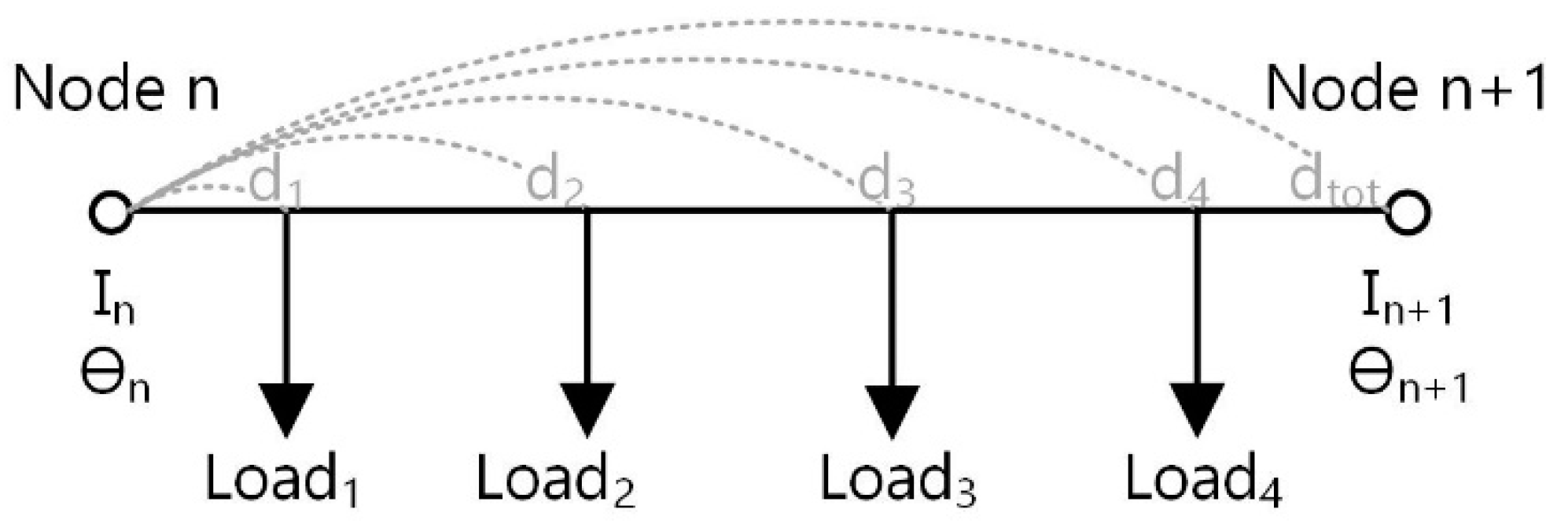
2.2.2. Studies on Voltage Estimation Based on Section Load Center

Park et al. proposed a voltage estimation method considering the distributed load based on the load center [16]. The load center is a virtual point at the load of a section and is assumed to be concentrated [25]. As illustrated in Figure 2, the section load center is obtained by calculating the average points of loads, which are distributed in sections, and aggregating them in a form of a concentrated load. A section load center is calculated based on the capacity of an equipment or the contract power information of high voltage load. The section load center is obtained by applying Equation (1) [25].

$$LC=\frac{{\sum }_{k=1}^m\left(d_k\ast L_k\right)}{{\sum }_{k=1}^m{L}_k},$$

(1)

where m denotes the total number of loads between node n and node n + 1, $d_k$ denotes the ratio (0~1) of the distance from node n to kth load among the total distance from the node n to the node n + 1. $L_k$ is the magnitude of the kth load.

This study assumed a fixed load center (FLC) calculated by using only static data like the equipment capacity or the contract power of high voltage customers. However, as the actual loads vary by time, the load center also changes, as indicated by the solid line of Figure 3a. The voltage drop changes when the section load center varies as shown in Figure 3b. Therefore, the estimation error is increased when the load center variation is not considered. Furthermore, voltage estimation was performed for the main feeder with loads only. However, the distribution network may include DGs and lateral feeders. Therefore, the effect of these elements needs to be considered.

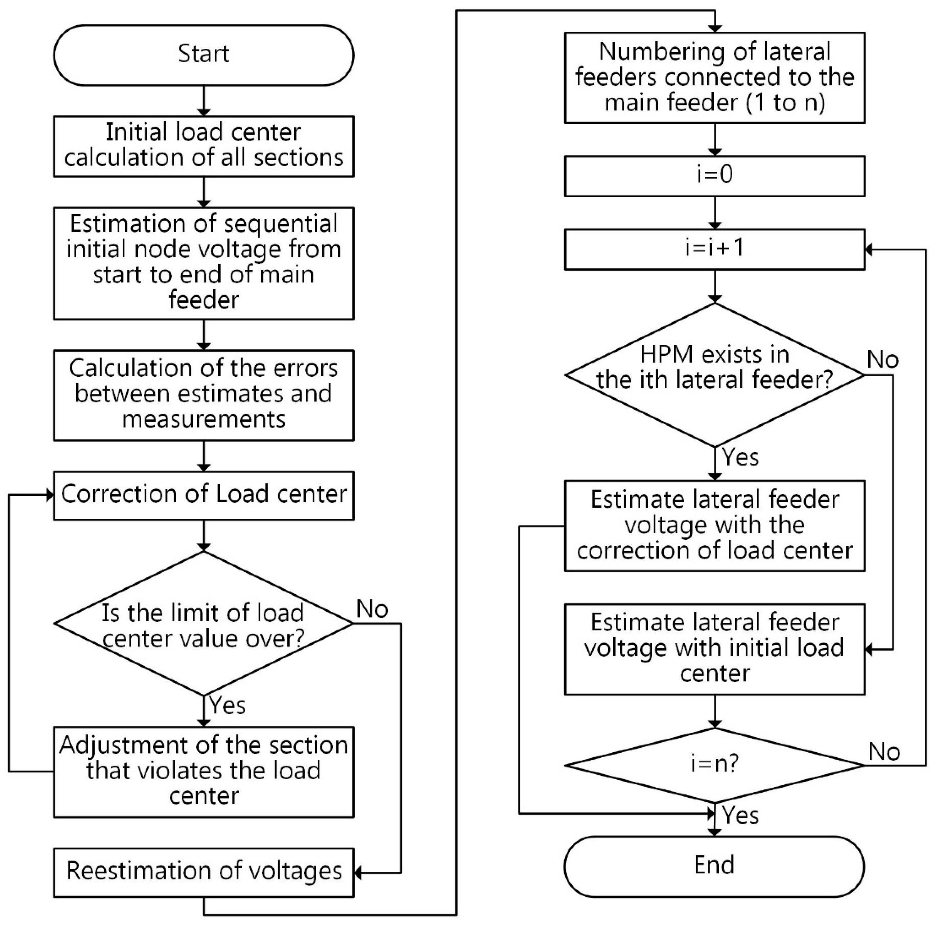
3. Proposed Voltage Estimation Method

As illustrated in Figure 4, there are multiple measurement devices in a distribution network. In recent years, PQ meter, PMUs, and other HPMs have been used more than ever before. The zone where high-precision voltage measurement at both ends of the main feeder through HPM or CVT of the substation is defined as the correctable zone. Inside the correctable zone, there are several sections divided based on the measurement units that cannot measure high-precision voltage, such as RTUs. In this section, the loads are irregularly distributed. The proposed estimation method consists of three steps. In step 1, section types are identified according to whether they are in the main or lateral feeder and whether there are only loads or DGs installed. The section types are classified into load dominant sections and generation dominant sections by using the measurement data, such as current magnitudes and voltage–current phase differences at both ends of each section. In step 2, the voltage of the main feeder is estimated by using the initial section load center and measurements data. If the estimated values and voltage measurements of the HPMs do not match, a correction parameter of the section load center is calculated. Then, the voltage of each section is estimated again by considering the correction parameter of the section load center according to the section types. If there are additional HPMs in the correctable zone, the estimation accuracy can be further improved. After that, the voltages of the nodes in the lateral feeder are approximately calculated based on the voltage estimation of the main feeder. In step 3, the active and reactive powers at both ends of the section are calculated by using voltage estimation. The line loss within a section is calculated by a corrected section load center and measurement data. Thus, the section loads are calculated. If there are lateral feeders within a section, the section loads are distributed to complete the estimation.

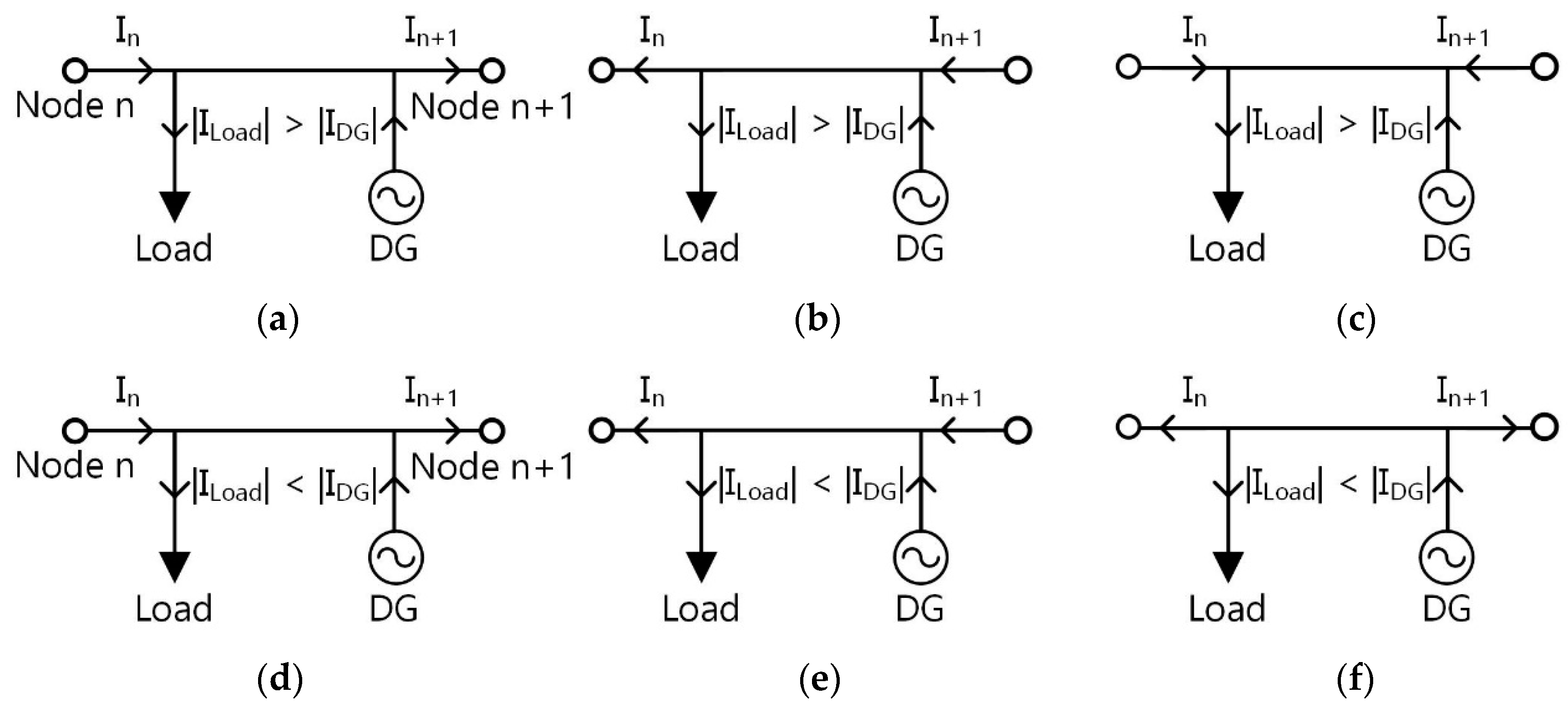
3.1. Step 1: Identification of Section Types Using Measurement Data

As mentioned above, this study corrects the section load centers for voltage estimation. Here, the section types need to be distinguished since the voltage drop characteristics are different due to the change of power flow direction. In the radial distribution network, where no DG exists, or the DG has a small capacity, the current flow has behavior as illustrated by Figure 5a. On the other hand, if the number and capacity of DGs are increased, the current flow of a section has one of the six behaviors according to the DG power output and load. If the section load center is corrected without considering the type of section, the correction will be wrong. This study classifies sections into two types: load dominant and generation dominant sections. In this study, the division between the load and the generation dominant section is distinguished by the magnitude of the current flowing through both ends of the section and the voltage–current phase difference. By taking cosine on the voltage–current phase difference, the current direction can be obtained. This direction information and the current magnitude at each end of the section can be used to determine if the current is supplied or absorbed in this section. If it is a section that absorbs current, it is categorized into the load dominant section and if it is a section that supplies current, it is categorized into the generation dominant section. The load dominant section is the one where the power consumption of loads is larger than the power output of generators. There are three types of load dominant sections, as illustrated in Figure 5a–c. When the current flows in the same direction at both ends, and if the magnitude of the current at the sending end is larger than the one at the receiving end, the section becomes a load dominant section (Figure 5a,b). If the current flowing at both ends is directed towards the inside of a section, the section is a load dominant section (Figure 5c). The generation dominant section is the one where the power output of generators is larger than the power consumption of loads. As shown in Figure 5d–f, there are three types of generation dominant sections. When the current flows in the same direction at both ends and if the magnitude of current at the sending end is less than that at the receiving end, the section is a generation dominant section (Figure 5d,e). If the currents of both ends are directed towards the outside of the section, it is a generation dominant section (Figure 5f).

3.2. Step 2: Calculation of Correction Parameter of the Section Load Center and Voltage Estimation

Figure 6 shows the flowchart of the proposed voltage estimation. In the first step, the initial load centers of each section are calculated by using Equation (1). Figure 7 shows an equivalent circuit of a distribution line. Vector values are marked with and the other values are scalar values. Therefore, $\dot{E_s}$ is the voltage vector of the sending end, $\dot{E_r}$ is the voltage vector of the receiving end, and $\dot{I}$ is the current vector flowing in the line. The equation for calculating the voltage magnitude of $\dot{E_r}$ is shown in Equation (2) [25].

$$E_r=E_s-I\left(Rcos{\theta }_r+Xsin{\theta }_r\right),$$

(2)

where $E_s$ is the magnitude of the sending end voltage, $E_r$ is the magnitude of the receiving end voltage, $I$ is the magnitude of current, ${\theta }_r$ is the phase difference between the voltage and current at the receiving end, and $R,X$ are the line impedances. In the network where the load is located in the section as shown in Figure 8, there are two types of currents: the current $I_{n+1}$ flowing from node n to node n + 1 and the current $I_n-I_{n+1}$ flowing from node n to the load. Therefore, considering $L{C}_{init}$ is the ratio of the load center position (between 0 and 1) to the total length of the line, the voltage drop by each current can be calculated as follows.

$$\begin{gathered} E_{Drop1}=I_{n+1}\left(Rcos\theta +Xsin\theta \right) \\ {E}_{Drop2}=L{C}_{init}\left(I_n-I_{n+1}\right)\left(Rcos\theta +Xsin\theta \right), \end{gathered}$$

(3)

where $E_{Drop1}$ is the voltage drop from the current $I_{n+1}$ and $E_{Drop2}$ is the voltage drop from the current $I_n-I_{n+1}$. Therefore, the voltage of node n + 1 can be calculated by the following equation [16].

$$\begin{array}{ll}{E}_{n+1, est}& =E_n-I_{n+1}\left(Rcos\theta +Xsin\theta \right)-L{C}_{init}\left(I_n-I_{n+1}\right)\left(Rcos\theta +Xsin\theta \right)\\ & =E_{n,est}-\left(I_{n+1}+L{C}_{init}\times \left(I_n-I_{n+1}\right)\right)\left(Rcos\theta +Xsin\theta \right),\end{array}$$

(4)

where $E_{n,est}$ is the initial estimated voltage value at the nth node, and $I_n$ is the current measured at the nth node. R and X are the line resistance and reactance of a section, and $\theta$ is the measured voltage–current phase difference. $L{C}_{init}$ is the initial load center. This equation is based on the assumption that the power flows in one direction in a load-only distribution network, where the gap of the voltage–current phase difference between node n and node n + 1 is small. However, when DGs are interconnected to the distribution system, the direction of the power flow is changed, and the phase difference between node n and node n + 1 may increase by more than 180°. Therefore, as shown in Equation (5), the voltage drop of each line should be calculated based on the load center. In the case of the left side based on the section load center in Figure 8, the voltage drop is calculated by using the impedance until the section load center among the total impedance of the section and the current and voltage–current phase difference measured at node n. In the case of the right side, the voltage drop is calculated by subtracting the impedance to the section load center from the total impedance of the section and current and voltage–current phase difference measured at node n + 1. For these reasons, the initial voltage is estimated using Equation (5).

$$\begin{array}{ll}{E}_{n+1,est}=& E_{n,est}-(I_n\times L{C}_{init}\times \left(Rcos{\theta }_n+Xsin{\theta }_n\right)\\ & +I_{n+1}\times \left(1-L{C}_{init}\right)\times \left(Rcos{\theta }_{n+1}+Xsin{\theta }_{n+1}\right))\end{array}$$

(5)

If an HPM exists at the end of a feeder, the error between the estimated voltage using Equation (5) and the precise measurement of the HPM can be known, and should be corrected. In addition, the section types mentioned above should be considered for this correction. In order to perform the voltage estimation using the correction of the load center, the load dominant section is aggregated to a single load as shown in Figure 9a and the generation dominant section is aggregated to a single generator as shown in Figure 9b. We estimate voltages sequentially from the start point to the end of the main feeder. It is necessary to consider whether the voltage rises or drops at the (n + 1)th node based on the nth node according to the change of the load center.

As illustrated in Figure 5, the current flow of a section has one of six behaviors. In the load dominant section, the current at both ends of the section can flow in three behaviors as shown in Figure 5a–c. If the current behaviors at both ends of the load dominant section, as shown in Figure 9a, are equal to Figure 5a, then the load center ${LC}_L$ moves to the right and the large current $I_n$ flows to the longer section. Therefore, the voltage drop increases, so that the voltage of the node n + 1 will be lowered. In the section that has the current behavior as shown in Figure 5b, as the load center ${LC}_L$ moves to the right, the larger current $I_{n+1}$ flows to the shorter section, and the voltage rise decreases. Therefore, the voltage at node n + 1 will be lowered. If the current behavior is like Figure 5c, then as the section load center ${LC}_L$ moves to the right, the current $I_n$ flows to the longer section; thereby the voltage of the node n + 1 will be lowered. Therefore, in the load dominant section, the voltage of the node n + 1 decreases as the section load center moves to the right (${LC}_L\to {LC}_L^{\prime }$) regardless of the current behaviors.

In the generation dominant sections, the current at both ends of the section can flow in three behaviors as shown in Figure 5d–f. If the current behaviors at both ends of the generator dominant section, as shown in Figure 9b, are equal to the one shown in Figure 5d,e, then the magnitude of $I_n$ and $I_{n+1}$ are opposite to those of Figure 5a,b. For this reason, as the load center moves right, the voltage of the node n+1 will be raised. In the current behavior, as shown in Figure 5f, as the section load center ${LC}_{DG}$ moves to the right, the current $I_{n+1}$ flows to the longer section; thereby the voltage of the node n + 1 is raised. Therefore, in the generation dominant section, as shown in Figure 9b, the voltage of the node n + 1 increases as the section load center moves to the right (${LC}_{DG}\to {LC}_{DG}^{\prime }$).

This characteristic of voltage variation should be considered to correct the section load center. Moreover, since the section load center needs to be located between both ends of the section, the load center should be corrected within the section.

In this paper, the correction parameter of the section load center is defined as ${\alpha }_{LC}$ which is calculated to eliminate the error between the voltage estimation obtained by Equation (5) and the voltage measurement at the node where an HPM is installed. In order to find ${\alpha }_{LC}$, Equation (6) can be obtained by substituting $L{C}_{init}$ → $L{C}_{init}+{\alpha }_{LC}$ of Equation (5) for the load dominant section. Since the voltage drop according to the movement of load center between the load and generation dominant sections is the opposite, the voltage estimation of the generation dominant section can be obtained as shown in Equation (7).

$$\begin{array}{r}{E}_{n+1,est}^{\prime }=E_{n,est}^{\prime }-\left(I_n\times (L{C}_{int}+{\alpha }_{LC}\right)\times \left(Rcos{\theta }_n+Xsin{\theta }_n\right)\\ +I_{n+1}\times \left(1-L{C}_{int}-{\alpha }_{LC}\right)\times \left(Rcos{\theta }_{n+1}+Xsin{\theta }_{n+1}\right))\end{array}$$

(6)

$$\begin{array}{r}{E}_{n+1,est}^{\prime }=E_{n,est}^{\prime }-\left(I_n\times (L{C}_{int}-{\alpha }_{LC}\right)\times \left(Rcos{\theta }_n+Xsin{\theta }_n\right)\\ +I_{n+1}\times \left(1-L{C}_{int}+{\alpha }_{LC}\right)\times \left(Rcos{\theta }_{n+1}+Xsin{\theta }_{n+1}\right)),\end{array}$$

(7)

where $E_{n,est}^{\prime }$ is the estimated voltage value considering ${\alpha }_{LC}$ for the node n. The voltage at the node m with an HPM is obtained by subtracting all the voltage drops until the end of the line in the section from the voltage at the start point of the feeder. Equation (8) is used to calculate ${\alpha }_{LC}$, which equates the estimated voltage value $E_{m,est}^{\prime }$ to the measurement $E_{m,meas}^{\prime }$ in node m.

$$\begin{array}{ll}{E}_{m,meas}^{\prime }& =E_{m,est}^{\prime }\\ & =E_{1,meas}-\sum _{ST\in Load}(I_n\times \left(L{C}_{ini{t}_{n,n+1}}+{\alpha }_{LC}\right)\times {\beta }_n+I_{n+1}\times \left(1-L{C}_{ini{t}_{n,n+1}}-{\alpha }_{LC}\right)\times {\beta }_n\\ & +I_{n+1}\times \left(1-L{C}_{ini{t}_{n,n+1}}-{\alpha }_{LC}\right)\times {\beta }_{n+1})-\sum _{ST\in DG}(I_n\times \left(L{C}_{ini{t}_{n,n+1}}-{\alpha }_{LC}\right)\\ & \times {\beta }_n+I_{n+1}\times \left(1-{LC}_{{init}_{n,n+1}}+{\alpha }_{LC}\right)\times {\beta }_{n+1})\\ & =E_{1,meas}-\sum (L{C}_{init}{}_{n,n+1}\times \left(I_n\times {\beta }_n-I_{n+1}\times {\beta }_{n+1}\right)+I_{n+1}\times {\beta }_{n+1})\\ & -{\alpha }_{LC}\times (\sum _{ST\in Load}\left(I_n\times {\beta }_n-I_{n+1}\times {\beta }_{n+1}\right)-\sum _{ST\in DG}\left(I_n\times {\beta }_n-I_{n+1}\times {\beta }_{n+1}\right))\\ & =E_{1,meas}-E_{m,est}\\ & -{\alpha }_{LC}\times (\sum _{ST\in Load}\left(I_n\times {\beta }_n-I_{n+1}\times {\beta }_{n+1}\right)-\sum _{ST\in DG}\left(I_n\times {\beta }_n-I_{n+1}\times {\beta }_{n+1}\right)),\end{array}$$

(8)

where $L{C}_{init}{}_{n,n+1}$ is the initial section load center between node n and n + 1. ${\beta }_n$ is the $Rcos{\theta }_n+Xsin{\theta }_n$ of the node n, and ST denotes each section type. In Equation (8), the constant term except ${\alpha }_{LC}$ on the right side is equal to the initial voltage estimate of the node m. Accordingly, if all the values except ${\alpha }_{LC}$ are put from the right side to the left side, an estimation error is obtained, as expressed in Equation (9). If Equation (9) is arranged with respect to ${\alpha }_{LC}$, the section load center can be expressed by using Equation (10).

$$E_{m,meas}^{\prime }-E_{m,est}={\alpha }_{LC}\times ({\sum }_{ST\in DG}\left(I_n\times {\beta }_n-I_{n+1}\times {\beta }_{n+1}\right)-{\sum }_{ST\in Load}\left(I_n\times {\beta }_n-I_{n+1}\times {\beta }_{n+1}\right))$$

(9)

$${\alpha }_{LC}=\frac{E_{m,meas}^{\prime }-E_{m,est}}{{\sum }_{ST\in DG}\left(I_n\times {\beta }_n-I_{n+1}\times {\beta }_{n+1}\right)-{\sum }_{ST\in Load}\left(I_n\times {\beta }_n-I_{n+1}\times {\beta }_{n+1}\right)}$$

(10)

When ${\alpha }_{LC}$ obtained by using Equation (10) is substituted in Equations (6) and (7), the voltage estimates of each node can be calculated with the section load center being corrected. The voltage for the lateral feeder can be estimated if it is interconnected to the main feeder with RTUs. The voltage of the lateral feeder is estimated by using the estimated voltage value at the node before the lateral feeder branches off from the main feeder. In case the HPM is installed at the end of a lateral feeder, the voltage estimation with the section load center corrected by the ${\alpha }_{LC}$, is conducted by using Equations (5)−(10). In case there is no HPM, the voltage estimation with fixed load center is performed by using Equation (5).

3.3. Step 3: Section Load and Loss Calculation

After the voltages at both ends of each section are estimated, the section load is calculated by using the voltage estimation. For the calculation of the section load, the active and reactive powers flowing in each node are calculated based on the voltage estimation, current magnitude, and voltage–current phase differences. Then, the losses caused by currents flowing in each line are calculated by using Equation (11). The conventional method sets up an equation under the assumption that the section load center is located at the middle of the section including only loads. For this reason, the line loss was calculated by using a simple formula $P_{loss}=3\times I^2\times R$, which includes the average value of currents measured at both ends of the section [15]. However, the section load center moves in real time, and the current may flow bidirectionally due to the DGs. Therefore, this study proposes a method of calculating line loss at both ends by considering the section load center, as expressed in Equation (11).

$$\begin{gathered} P_{los{s}_{n,n+1}}=3\times \left({\left(I_n\right)}^2\times L{C}_{new}{}_{n,n+1}\times R_{n,n+1}+{\left(I_{n+1}\right)}^2\times \left(1-L{C}_{new}{}_{n,n+1}\right)\times R_{n,n+1}\right) \\ {Q}_{los{s}_{n,n+1}}=3\times \left({\left(I_n\right)}^2\times L{C}_{new}{}_{n,n+1}\times X_{n,n+1}+{\left(I_{n+1}\right)}^2\times \left(1-L{C}_{new}{}_{n,n+1}\right)\times X_{n,n+1}\right), \end{gathered}$$

(11)

where $P_{los{s}_{n,n+1}}$, $Q_{los{s}_{n,n+1}}$ are the loss of active and reactive powers between the nth and (n + 1)th nodes. ${LC}_{new}{}_{n,n+1}$ is the section load center between the nth and (n + 1)th nodes, which is corrected by ${\alpha }_{LC}$. The section load considering the losses can be calculated as in Equation (12).

$$P_{loa{d}_{n,n+1}}=P\left(n\right)-P\left(n+1\right)-P_{los{s}_{n,n+1}}{Q}_{loa{d}_{n,n+1}}=Q\left(n\right)-Q\left(n+1\right)-Q_{los{s}_{n,n+1}}$$

(12)

In the case of the generation dominant sections, the active and reactive powers flowing in each node are calculated with a negative sign due to the voltage–current phase difference. For this reason, the power output of each section is calculated as negative.

As shown in Figure 10, the loads are distributed in a section with a lateral feeder where the RTU is installed. As the active and reactive powers flow in each node, the section load center and section loads are already known through the analysis of a straight line, and only the position and magnitude of each load need to be calculated. A straight line section is divided into two sections, and the load center of the straight line section is applied at the load centers of the divided sections. Then, the magnitudes of the two loads are calculated by using Equations (13) and (14) to ensure that the values are the same as the load centers of the straight section, which is not divided before.

$$\frac{l_1\times LC\times L_1+\left(l_1+l_2\times LC\right)\times L_2}{L_{tot}}=LC,$$

(13)

$$L_1+L_2=L_{tot},$$

(14)

where, $l_1$ and $l_2$ denotes the ratio (0~1) of the distance from node n and node n + 1 to lateral feeder among the total distance from the node n to the node n + 1, respectively. As all the values, except $L_1$ and $L_2$, in Equations (13) and (14) are known, $L_1$ and $L_2$ can be obtained by solving the simultaneous equations.

4. Case Study

Case studies were performed by test systems. Three phase radial distribution networks were implemented. ACSR of 160 ${\mathrm{mm}}^2$ with the impedance of (0.1823 + j.0.3901) Ω/km was used for the line of 22.9 kV distribution network. The number of RTUs installed in the topology of the test model was determined according to the Korean switch installation regulations [26].

A total of four case studies were carried out. For each case study, selective comparisons were performed between the estimation methods that use a fixed load center (FLC method [16]), a method using the state estimation (IRWLS method [14]), and the proposed method in this study. Since both the proposed method and the FLC method use the measured values at the switch, the current through the switch by assumed load and PV were extracted using Simulink, and the voltage and load were estimated using a program implemented in MATLAB. To conduct a simulation using the IRWLS method, K-mean clustering was implemented in MATLAB, and the IRWLS used a Pandapower tool (a Python-based tool) [27]. The estimation was conducted by using the voltage and active/reactive power of the substation measured using Simulink and the estimated load and PV output values obtained by using K-mean clustering as input values of the IRWLS. In order to perform state estimation using the IRWLS of Pandapower, a standard deviation of the measurement error is required. For the voltage and active/reactive power of the substation, a standard deviation is assumed ${10}^{-8}$ and the standard deviation of load and PV used are 0.02 and 0.5, respectively.

In case study 1, voltage estimation by three methods was compared for a simple distribution system. To conduct the comparison, the actual load measurement data presented elsewhere [28] were used as load values. As the training data for K-mean clustering of the IRWLS method, the data from 29 June to 3 July were used. For the test data, load data from 6 July were used. For the PV power generation, an actual output data of 250 kW PV (on Building No. 5 of College of Engineering at Chonnam National University, South Korea) from 29 July to 2 August were used as training data, and the data from 5 August were used as the test data. The PV output measurement data used for training and the test data are shown in Figure 11. Case study 2 analyzed how the estimated error of the previous node affects the voltage estimation of the next node for the linear section network of case study 1. The simulation of the estimated error accumulation of the conventional method and the proposed method was performed. In case study 3, the estimated error of the proposed method was analyzed according to the number of HPM installations for networks with multiple lateral feeders and PVs similar to the actual distribution network. In case study 4, the network of case study 3 was simulated for the measurement noises that could occur in actual network operation. The simulation was performed by applying the load and PV profile used in case study 1. In addition, to analyze the estimation errors of the proposed method and the existing methods, according to measurement errors, the estimation results of the proposed method and the FLC method were derived by applying 1–5% of the normally distributed noise to the current measurements. The estimation result of the IRWLS method was derived by applying 1–2% of the normally distributed noise to the load measurements. Finally, the estimation errors of each method were compared with each other.

4.1. Case 1: Simple Radial Distribution System with One DG

To compare the estimation results of the conventional and proposed method, a simulation was performed for the test system illustrated in Figure 12. It consists of five sections all in the main feeder without lateral, and it was assumed that only one DG is installed in the feeder. The input data are as shown in

Table 2. Input and measurement data of case study 1.

Section No.	From Node	To Node	Line		Section Load			Initial Load Center
			No.	Length (km)	No.	Active Power (kW)	Reactive Power (kVar)
1	1	2	1	1.177	1 2 3	956.3 141.8 476.8	463.1 68.7 230.9	0.631
			2	0.459
			3	1.351
			4	1.013
2	2	3	1	1.154	1 2 3	778.0 770.1 729.2	376.8 373.0 353.1	0.735
			2	1.410
			3	0.356
			4	1.08
3	3	4	1	1.381	1	228.3	110.5	0.795
			2	0.772	2	817.7	396.0
			3	1.233	3	−29,709.2	140.8
			4	0.614		(PV)
4	4	5	1	1.684	1 2 3	356.4 219.1 628.6	172.6 106.1 304.4	0.951
			2	0.775
			3	1.162
			4	0.379
5	5	6	1	0.589	1 2 3	701.9 756.9 147.5	339.9 366.6 71.4	0.431
			2	1.053
			3	0.784
			4	1.574

. An HPM was installed at the end of the line, and RTUs were installed at each node. The length of each section was 4 km and the impedance of the section was 4 × (0.1823 + j.0.3901 Ω/km). It was assumed that each section was composed of three distributed loads and/or DGs where the length between loads and the magnitude of loads and DGs were arbitrarily chosen. The simulation was carried out by applying the previously mentioned actual measured load and the PV output profile to each load and PV.

The estimation errors of each method for 24 h are listed in

Table 3. Comparison of voltage and load estimation accuracy of fixed load center (FLC) method, iteratively re-weighted least square (IRWLS) method, and proposed method.

Method	Voltage Estimation Error			Load Estimation Error
	Average (%)	Maximum (%)	Standard Deviation	Average (%)	Maximum (%)	Standard Deviation
FLC Method	0.1037	0.3228	0.0801	0.1800	1.6618	0.2303
IRWLS Method	0.0153	0.0464	0.0101	6.1981	193.85	19.781
Proposed Method	0.0088	0.0457	0.0096	0.1258	1.1968	0.2308

. The proposed method was shown the smallest estimation error in both voltage and load estimations. It obtained an average error of 0.0088% and a maximum error of 0.0457% for the voltage estimation and an average error of 0.1258% and a maximum error of 1.1968% for the load estimation. For the result of voltage estimation, the FLC method had the lowest accuracy for the voltage estimation with an average error of 0.1037% and a maximum error of 0.3228%. The true and estimated voltage value of the FLC, IRWLS, and proposed methods at node 4 are shown in Figure 13. The results of the proposed method and IRWLS method were similar to the true value, but the FLC method had a significantly bigger estimation error than the other methods. The IRWLS method could estimate more accurately using measurement data of individual loads, and the proposed method enabled accurate estimation through section load correction using the HPM. However, the FLC method showed a large estimation error compared to other methods because there was no measurement of individual loads or correction of estimation errors. In case of the load estimation, the IRWLS method had the lowest accuracy for the load estimation with an average error of 6.1981% and a maximum error of 193.8%. When a load estimation error of 193.8% occurred at 17:00, the actual load of Section 3 was 65.6 kW, while the IRWLS method estimated the load to be 192.8 kW. The absolute magnitude of error was small at approximately 127.2 kW, but the error rate was significantly large at 193.8%. In the process of the K-mean clustering, which generates load and PV input data of IRWLS, the deviation of the input value is large because of the variation value of the PV output is larger than that of the load. Results of load estimation for Section 3 and Section 4 by each method are shown in Figure 14. As mentioned above, Section 3, where PV is interconnected, is the generation dominant section with a large PV, and the IRWLS method had the lowest estimation accuracy than the other methods owing to the change in PV output. However, in Section 4, where only the loads existed, all three methods had similar accuracy.

4.2. Case 2: Impact of Estimation Error Accumulation

The analysis of which node’s estimation error has the cumulative effect of the error in calculating the next node’s estimate is an important factor to verify the practical applicability of the proposed method. To this end, we added an error to node 1 of the test network in case 1 and analyzed how it affects the voltage estimation of other nodes. Figure 15 shows the simulation results of the existing method and the proposed method for the propagation of the cumulative error. As a result of adding the estimation error of 0.1–0.5%, the estimation error of the previous node was accumulated as it is, and the estimation error of the next node tended to increase when the existing method was used. In the case of the proposed method, when the estimation error of the previous node occurs, the estimation error of the next node eventuates. However, it can be observed that there was no accumulation of the effect towards the end of the feeder. These results were obtained because the estimation error was corrected through the HPM.

4.3. Case 3: Radial Distribution System with Multiple DGs and Lateral Feeder

The test system of Figure 16 was used to evaluate the effects of multiple DGs and lateral feeder both in the proposed method and in the conventional method. The test system model is based on an actual Korean distribution network [26] and its parameters are as shown in

Table 4. Input data of case study 2.

Section No.	From Node	To Node	Line		Section Load			Initial Load Center	Changed Load Center
			No.	Length (km)	No.	Active Power (kW)	Reactive Power (kVar)
1	1	2	1	0.123	1 2 3	66.7 109.0 37.3	25.1 51.0 13.6	0.368	0.152
			2	0.323
			3	0.240
			4	0.114
2	2	3	1	0.715	1 2 3	344.7 453.0 247.2	140.1 217.2 95.0	0.616	0.401
			2	0.790
			3	0.944
			4	0.751
3	3	4	1	1.122	1 2 3	37.9 858.5 590.9	15.0 253.6 227.7	0.727	0.511
			2	1.035
			3	0.382
			4	0.660
4	4	5	1	0.84	1 2 3	394.7 878.1 4.7	160.4 383.4 2.1	0.956	0.740
			2	1.124
			3	0.598
			4	0.638
5	5	6	1	0.280	1	117.4	49.8	-	-
			2	0.774	2	372.0	147.4
			3	0.244	3	24.2	11.60
			4	0.301	4	−1000.0 (PV)	0
6	7	-	1	0.237	1	71.1	23.4	0.450	0.235
			2	0.110	2	196.6	94.6
			3	0.608	3	620.6	290.0
7	8	9	1	0.255	1	173.0	59.1	0.342	0.127
			2	0.810	2	416.8	142.2
			3	0.611	3	315.9	135.9
			4	0.725	4	−1000.0 (PV)	0
8	10	11	1	0.979	1 2 3	247.9 411.6 82.5	86.7 178.3 27.1	0.549	0.333
			2	0.918
			3	0.139
			4	0.363
9	11	12	1	1.333	1 2 3	220.5 115.4 578.0	103.1 54.0 242.9	0.314	0.098
			2	0.821
			3	0.527
			4	0.519
10	12	-	1	0.087	1	60.3	23.8	-	-
			2	0.248	2	63.7	23.5
			3	0.235	3	197.5	83.3
11	13	14	1	0.131	1	164.3	56.6	0.516	0.301
			2	0.905	2	95.0	40.5
			3	0.727	3	818.2	277.1
			4	0.637	4	−1000.0 (PV)	0

. At first, the voltage estimation errors were compared between the conventional method (no HPM) and the proposed method when one HPM was installed at node 6 (HPM #1). In order to analyze the effect of the number of HPMs on the estimation accuracy, the voltage estimation errors were observed by increasing the HPMs installed at nodes 12 (HPM #2), 9 (HPM #3), and 14 (HPM #4). Figure 17 shows each node voltage magnitude through the conventional method, proposed method, and the measurements. Compared to the conventional method, the proposed method estimates the voltage more accurately. Figure 18 presents the maximum voltage estimation error, average voltage estimation error, and standard deviation of errors obtained by the proposed method with different HPMs. When one HPM was installed at node 6, the average voltage estimation error was significantly reduced. When two HPMs were installed at nodes 6 and 12, the average and maximum voltage estimation errors remarkably decreased. When two other HPMs were installed additionally at nodes 9 and 14, the average and maximum voltage estimation errors decreased slightly.

4.4. Case 4: Presence of Current Measurement Noise

The causes of measurement uncertainty occurring in the actual distribution network can be largely divided into the measurement error of the sensor and the asynchronous that occurs in the process of collecting measurement information of the RTU to the DMS. Therefore, a noise injection test is important to verify the applicability to an actual network. Actual network data may be used for the test, but it is difficult to verify the accuracy of the methodology using the data with random noise. Therefore, in this study, the load and PV profiles used in case 1 are considered as the accurate value, and the true values of switch measurement and bus voltage were extracted through MATLAB simulation, and the noise was injected based on the international standards. For the test network, the network of case study 3 was used, and the estimated results of the FLC method, IRWLS method, and the proposed method were compared. However, it is difficult to consider the asynchronous of the measurement at the laboratory level, therefore the weight of the measurement error of the sensor was highly reflected. Regarding the range of the current magnitude measurement noise to be added, as the maximum noise of class 5 is set as ±5% [29], the current measurement noise was simulated with an incremental variation of 1% from ±1%~±5%. For the case of load measurements, simulations were conducted by injecting ±1% and ±2% of load measurement noise as the maximum noise was set to ±2% by class 2 [30]. The noise model was simulated by the normal distribution. The distribution was simulated for 1000 cases, and the results were analyzed with the mean, maximum, and standard deviation. The random noises were generated as many as “the number of nodes where the measuring instrument is installed × 1000” according to the noise model type. The noises were added to the measurement values by using the 1000 sets of noises generated as above and multiplying (1 + noise) PU to the measurement values of current magnitude for each simulation case. In order for the noise to be within the range with a confidence of 99%, in the case of 1% noise of the normal distribution simulation, the noise is generated so that the mean is 0 and 3σ is 0.01 PU. Furthermore, as mentioned above, the noise is multiplied by the measurement values of the current magnitude for simulation. Figure 19 shows the noise distribution. The value of the X-axis is the added noise, which is varied by 1% from ±1% to ±5% and simulated for a total of five cases. To show as the graphical form, the added noise for each case was treated in increments of 0.1%. For the case of ±2% (black solid line), the generated random noise is shown as 0.1% for +0.09% and −1.1% for −1.05%. The value on the Y-axis is the number of noises in the range. Therefore, Figure 19 is a graph of the number of noises corresponding to each range.

The voltage estimation errors of each method based on the measurement noise are shown in

Table 5. Comparison of voltage estimation accuracy of FLC method, IRWLS method, and proposed method.

Method	Noise	Voltage Estimation Error
		Average (%)	Maximum (%)	Standard Deviation
IRWLS Method	±0%	0.0236	0.1266	0.0231
	±1%	0.0237	0.1263	0.0231
	±2%	0.0235	0.1268	0.0230
FLC Method	±0%	0.0857	0.5377	0.1219
	±1%	0.0882	0.5194	0.1250
	±2%	0.0903	0.5406	0.1251
	±3%	0.0889	0.5285	0.1236
	±4%	0.0905	0.5824	0.1266
	±5%	0.0957	0.6210	0.1304
Proposed Method	±0%	0.0222	0.0853	0.0089
	±1%	0.0229	0.0857	0.0089
	±2%	0.0228	0.0830	0.0090
	±3%	0.0226	0.0942	0.0085
	±4%	0.0231	0.0976	0.0093
	±5%	0.0234	0.0982	0.0094

. Comparison of the current noise value of ±5% and the load noise value of ±2%, which are the maximum noise values assumed in the case study, indicates that the proposed method showed the highest estimation accuracy, whereas the FLC method showed the lowest estimation accuracy. When the results were compared with the noise-free case, the FLC method again showed the highest increase in the estimation error. When the proposed method was compared with the IRWLS method, both methods exhibited similar results in the case of average and maximum estimation errors.

The true voltage values at node 5 and the estimated values obtained by each method for the case of ±5% current measurement noise and ±2% load measurement noise are shown in Figure 20. The results obtained by the IRWLS method and the proposed method were approximately closer to the true value. However, the result obtained by the FLC method had a significantly large estimation error. The IRWLS method did not show a large increase in estimation error when injecting the normal distribution noise of 1%~2%. The WLS-based state estimation is a method that assumes random noise in the form of normal distribution, such as the form injected in this study, so the IRWLS method was not sensitive to normal distribution noise. In addition, the proposed method did not show a large increase in the estimation error, because the estimation error was corrected through the HPM even if there was a noise in the measured values. However, the estimation error of the FLC method was increased greatly because the measured value with the noise was used directly for estimation without any correction. From Table 5 and Figure 20, the proposed method was verified to provide higher estimation accuracy than the other methods even after the presence of noise in the measurements.

4.5. Summary of Case Studies

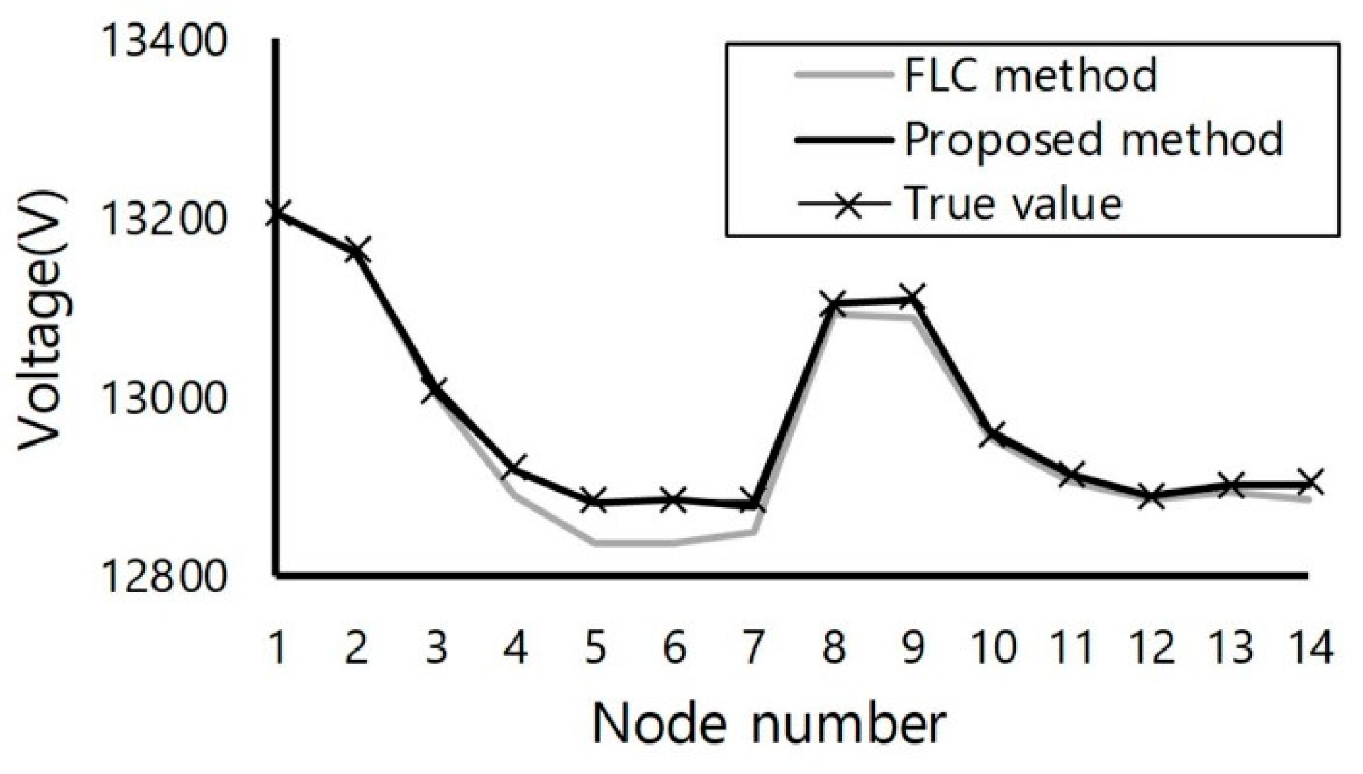
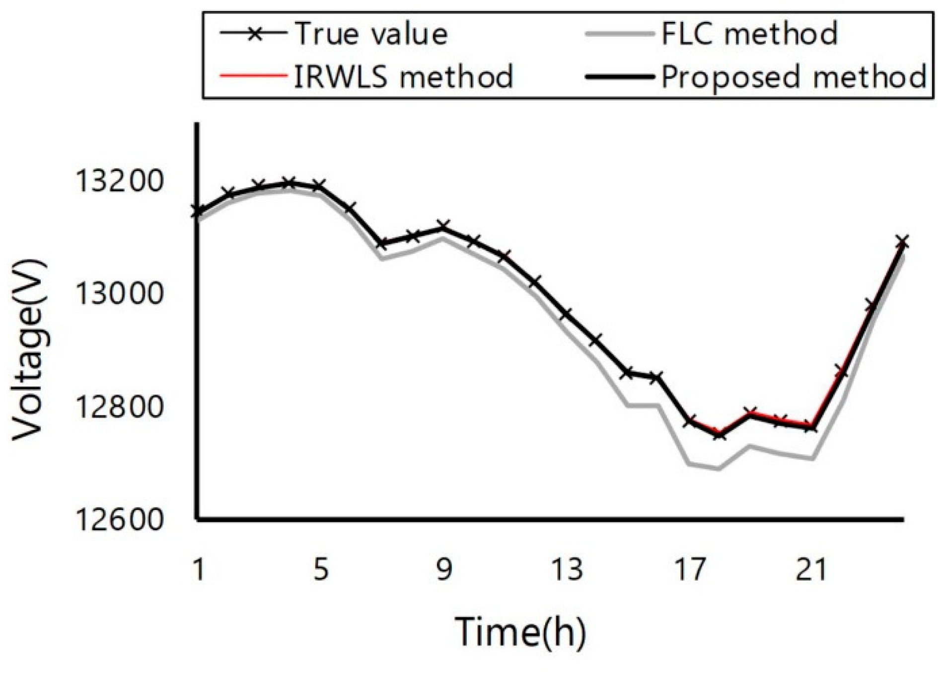
The results of case studies are summarized as follows.

(1)

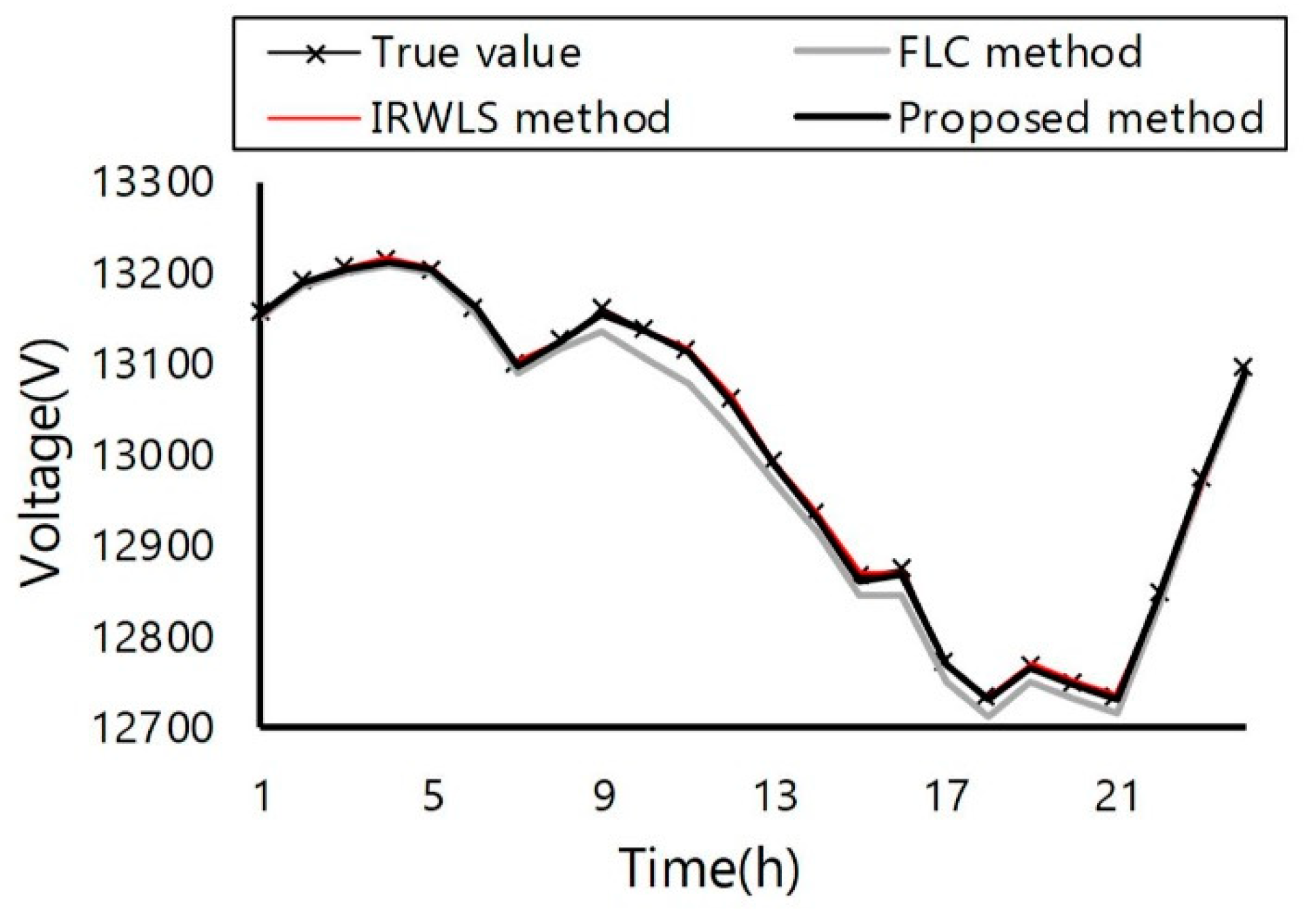
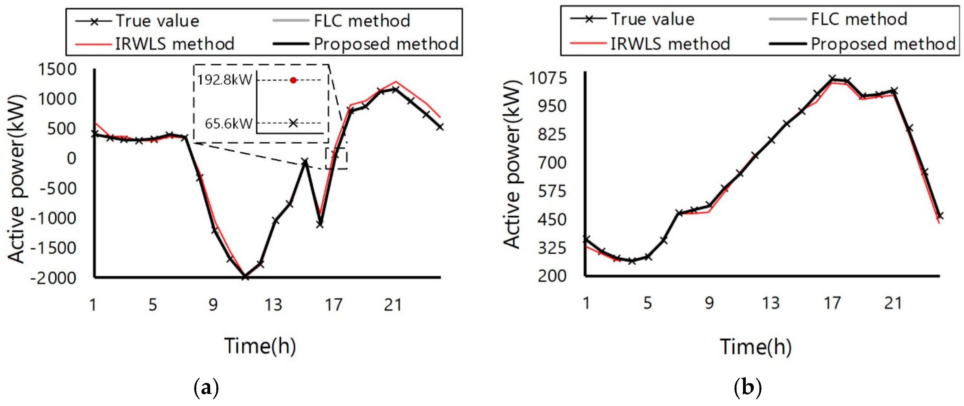
Comparison of the voltage estimation accuracy of the FLC, IRWLS, and the proposed method through case study 1 indicates that a significant improvement in the estimation accuracy of the proposed method was observed when compared with the FLC method and a slight improvement accuracy was observed when compared with the IRWLS method. Comparison of the load estimation accuracy shows that the proposed method had a significant improvement in the estimation error when compared with the FLC and IRWLS methods. The FLC method and IRWLS method were significantly affected by PV, so the accuracy of load estimation was low, but the proposed method was verified so that it was less affected by PV and showed more accurate estimation results than other methods.

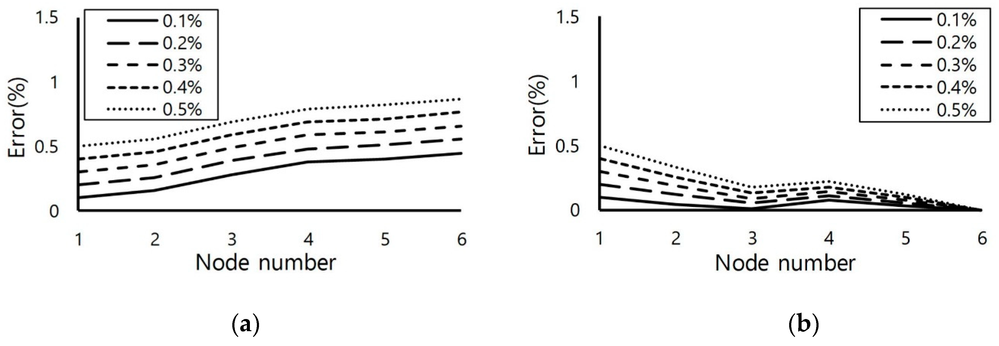
(2)

The proposed method performs sequential voltage estimation from the starting node to the end; therefore, the cumulative effect of the estimation error was analyzed in case study 2. In the FLC method, the estimation error of the previous node is accumulated as it is, and the estimation error of the next node increases. In the case of the proposed method, when the estimation error of the previous node occurs, the estimation error of the next node eventuates. However, it was confirmed that there was no accumulation of the effect toward the feeder end. These results indicate the robustness of the proposed method for the cumulative error propagation and its effectiveness for its application to the actual network.

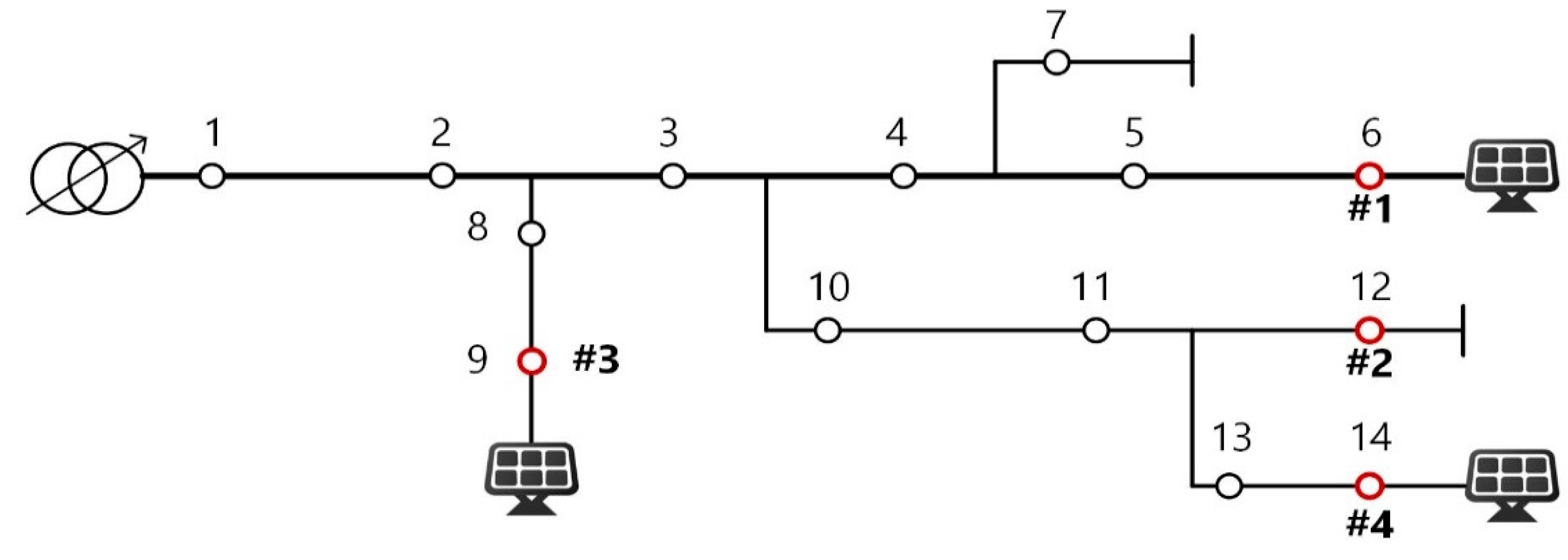
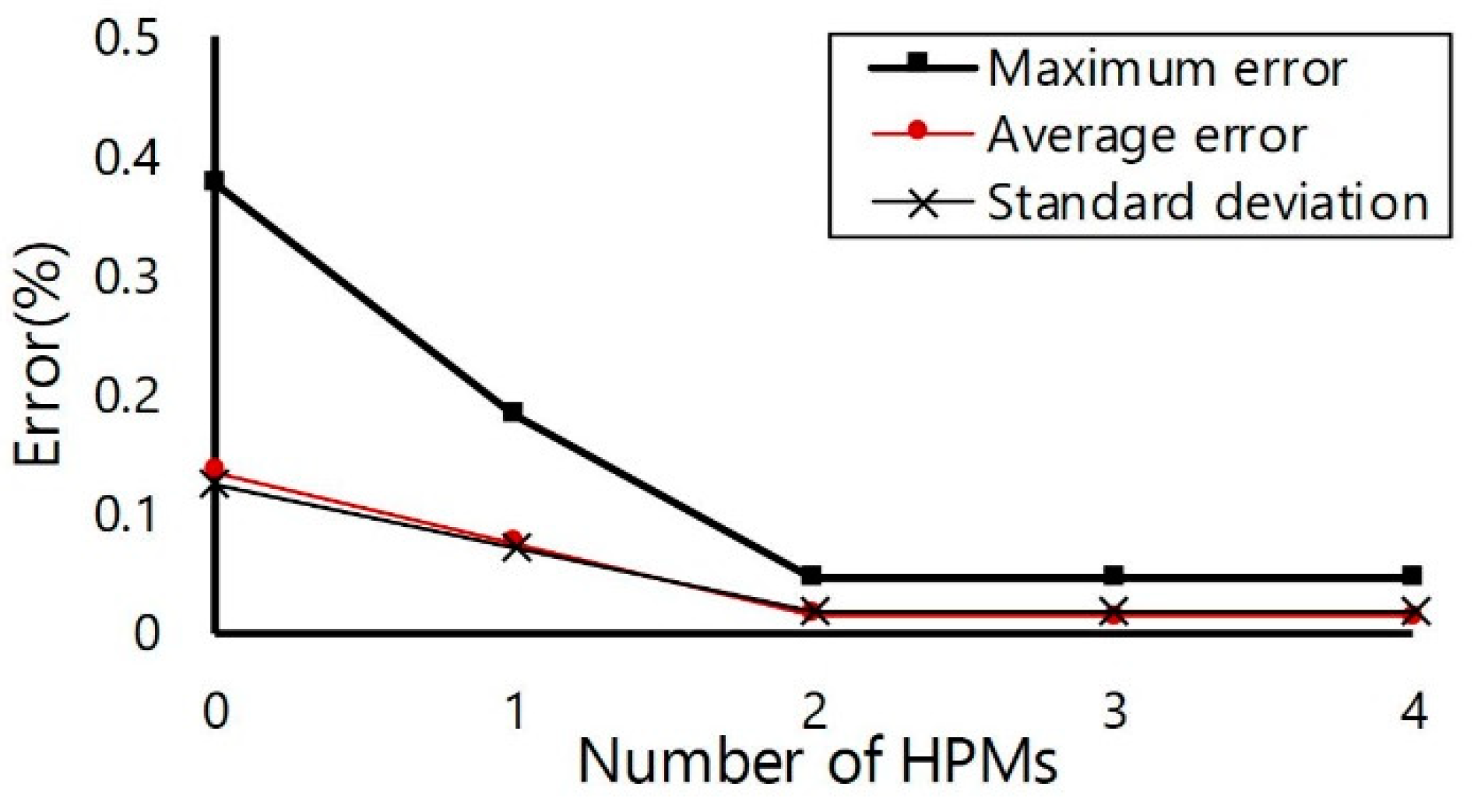
(3)

When the HPM is installed only at the end of the main feeder, it was confirmed that the estimation error increased as the length of the lateral feeder increased. For some cases, an additional HPM may be required for the long-distance lateral feeder. In case study 3, it was confirmed that, when an additional HPM was installed at the lateral feeder, the estimated error was significantly improved compared to the case where an HPM was installed only at the end of the main feeder. This can be viewed as a significant reduction in the error for the network of this case study. If the actual network for application is determined, the number of installed HPMs can be examined through simulation as in the case study in this paper. The final number of installations will be determined by combining requirements such as the estimation accuracy and installation costs desired by the utility company.

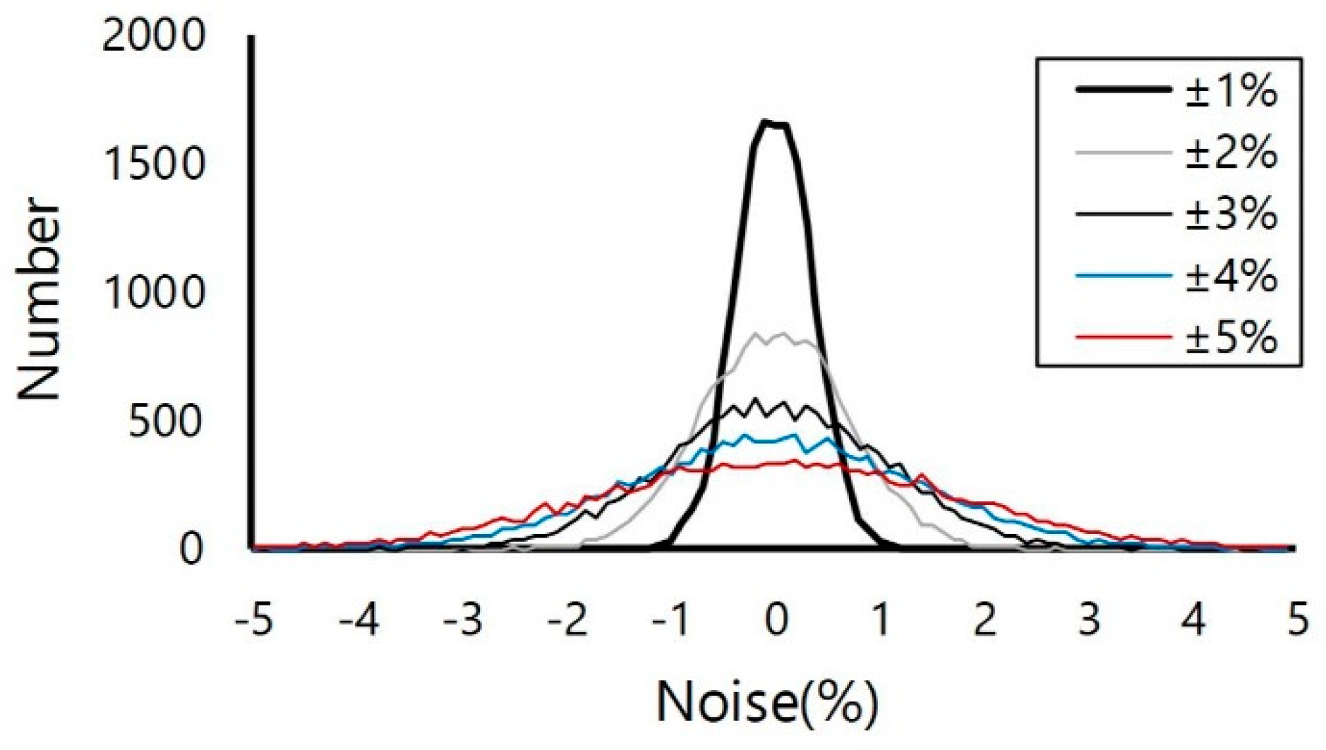
(4)

When the measurement noises were injected into each estimation method in case study 4, the proposed method showed robustness to noise. The result of voltage estimation simulation with measurement noise was that the proposed method had higher accuracy than the FLC and IRWLS methods. Therefore, the proposed method can provide an improved estimation accuracy compared to the existing methods even with the presence of measurement noises. This is a significant advantage of applying the proposed method to the actual distribution system.

In conclusion, verification of the proposed method was performed in a test model similar to an actual distribution network in this study, and through comparison with existing methods under the same conditions, the superiority of the proposed method can be summarized as follows. First, under the condition that PV is interconnected and there is no measurement noise, the existing methods were greatly affected by PV, and the estimation accuracy of voltage and load was low. Although the proposed method was less affected by PV, the estimation accuracy was more accurate. Second, the proposed method showed that the estimated error of the previous node had little effect on the next node, so the cumulative effect of the error was small. Third, under the presence of noise in the measurement values of the load and current, even in the case of maximum measurement noise, it was proven that the estimation accuracy of the proposed method was higher than other methods. These results show that the proposed method has a great advantage in the application of the actual network, considering the uncertainty of measurement and the recent trend that many PVs are interconnected to the distribution network.

5. Conclusions

In this paper, the voltage estimations in distribution networks were proposed. To overcome the limited applicability to actual distribution networks in the methods used in existing studies, this study considered the distributed loads in a distribution network and proposed a method of correcting the section load center through the measurements of HPMs. Even if only one HPM is installed, the accuracy of the voltage estimation of the main feeder can be greatly improved by the correction of the section load center. Through more accurate main feeder voltage, the estimation accuracy of the lateral feeder can also be greatly improved. By improving the voltage estimation accuracy, the section load can be calculated more accurately.

For the studies estimating voltage and load, verification of the proposed method through testing is very important. We believe that there are two types or stages of verification. The first one is for the proposed methodology itself; it verifies the validity of the formulas and the accuracy of the logic. At this stage, it is necessary to examine the problems of the methodology itself for the application in an actual network, and it is important to consider various factors such as measurement uncertainty and DGs. The second is to verify the applicability of the proposed method by installing in the operation system of an actual distribution network. This stage is not only to verify the methodology but also to check the various variables related to a distribution network and communication to increase its applicability when applying to the actual network.

In this paper, the first stage of verification of the accuracy of the methodology itself was performed. In this context, in order to consider two factors of measurement uncertainty such as the measurement error of the sensor and the asynchronous of the RTU, a noise test based on international standards was performed. Since the actual network measurements have random noises, it is difficult to know the true value, and it is difficult to use the actual data for the test input/output data at this stage. It is possible to obtain accurate data by installing metering out fit (MOF), etc. in the entire actual network, but this method is very difficult to implement at the laboratory level. Therefore, in this study, a noise injection test was performed using simulation-based true value as input/output data. Through the test, the proposed method was compared with previous studies and demonstrated methodological superiority. However, since it is difficult to consider the asynchronous of measurement at the laboratory level, much weight has been given on the measurement error of the sensor, and it is difficult that the study has included all factors of an actual network. Therefore, it is thought that the second stage of verification considering the uncertainty of measurement and environmental variables in the actual network needs to be performed as a further study in the future.

Despite the advantages of the proposed approach, the following aspects still need to be considered. First, as mentioned above, the voltage estimation method proposed in this paper is based on the correction of the estimation error by the HPM at the feeder end. Therefore, in the case of a long-distance lateral feeder without the HPM installed, the error of voltage estimation can only be increased. This may require additional installation of HPMs on long-distance lateral feeders and utility companies need to increase their installation and operation costs. However, the recent trend of grid modernization from increased distribution network interconnection of distributed generator is accompanied by the need to increase the installation of the new operating systems (ADMS, etc.) and new instruments for monitoring; such an additional installation of HPMs will not act as a major obstacle. Secondly, the purpose of the voltage estimation proposed in this paper is to estimate the voltage on the MV side for real-time operation of the network (voltage control, real-time network reconfiguration, etc.) at the DMS level. In general, the LV network, which is a consumer network and not the utility’s operating area, is not considered in this study. The estimation was performed based on the representative phase in this paper, but in the case of a three-phase unbalanced load, it can be considered if the estimation is performed with each phase as the representative phase. Thirdly, the proposed method aims to increase the precision of voltage and load estimation by adding only a minimum number of high-precision measurements to the network where the RTU is installed and operated. The proposed method is considered to be applicable to networks that apply automation of distribution networks (such as metropolitan networks in Korea, Japan, Hong Kong, Singapore, Asia, Europe, and North America) without significant additional cost. In addition, as mentioned above, grid modernization with the recent increase in the interconnection of distributed generator in distribution networks will lead to a gradual increase in the networks to which the proposed method can be applied.

References

1. McDonald, J. Adaptive intelligent power systems: Active distribution networks. Energy Policy 2008, 36, 4346–4351. [Google Scholar] [CrossRef]
2. Meliopoulos, A.P.S.; Polymeneas, E.; Tan, Z.; Huang, R.; Zhao, D. Advanced distribution management system. IEEE Trans. Smart Grid 2013, 4, 2109–2117. [Google Scholar] [CrossRef]
3. American National Standard for Electric Power Systems and Equipment Voltage Ratings (60 Hertz); NEMA ANSI C84.1-2011; ANSI: Washington, DC, USA, 2011.
4. Jin, T.H.; Chung, M.; Shin, K.Y.; Park, H.; Lim, G.P. Real-time dynamic simulation of korean power grid for frequency regulation control by MW battery energy storage system. J. Sustain. Dev. Energy Water Environ. Syst. 2016, 4, 392–407. [Google Scholar] [CrossRef] [Green Version]
5. Virk, A.K. Maximum Loading of Radial Distribution Networks. Master’s Thesis, Electrical and Instrumentation Engineering Department, Thapar University, Patiala, India, 2009. [Google Scholar]
6. IEC 61000-4-30: Testing and Measurement Techniques—Power Quality Measurement Methods; IEC: Geneva, Switzerland, 2012.
7. Characteristic of Metering Out Fit. Available online: http://www.transformadores.cl/en/project/3-elements-metering-outfit/ (accessed on 9 September 2019).
8. Micro-Synchrophasors for Distribution Grids. Available online: https://www.naspi.org/sites/default/files/2016-10/psl_mceachern_micro_synchrophasor_distribution_grid_20160323.pdf (accessed on 9 September 2019).
9. Ju, Y.; Wu, W.; Ge, F.; Ma, K.; Lin, Y.; Ye, L. Fast decoupled state estimation for distribution networks considering branch ampere measurements. IEEE Trans. Smart Grid 2018, 9, 6338–6347. [Google Scholar] [CrossRef] [Green Version]
10. Kong, X.; Chen, Y.; Xu, T.; Wang, C.; Yong, C.; Li, P.; Yu, A. hybrid state estimator based on SCADA and PMU measurements for medium voltage distribution system. Appl. Sci. 2018, 8, 1527. [Google Scholar] [CrossRef] [Green Version]
11. Muscas, C.; Pau, M.; Pegoraro, P.A.; Sulis, S. Uncertainty of voltage profile in PMU-based distribution system state estimation. IEEE Trans. Instrum. Meas. 2016, 65, 988–998. [Google Scholar] [CrossRef]
12. Muscas, C.; Sulis, S.; Angioni, A.; Ponci, F.; Monti, A. Impact of different uncertainty sources on a three-phase state estimator for distribution networks. IEEE Trans. Instrum. Meas. 2014, 63, 2200–2209. [Google Scholar] [CrossRef]
13. Yun, S.-Y.; Chu, C.-M.; Kwon, S.-C.; Song, I.-K.; Choi, J.-H. The development and empirical evaluation of the korean smart distribution management system. Energies 2014, 7, 1332–1362. [Google Scholar] [CrossRef] [Green Version]
14. Ali, A.-W.; Jianzhong, W.; Nick, J. State estimation of medium voltage distribution networks using smart meter measurements. Appl. Energy 2016, 184, 207–218. [Google Scholar]
15. Park, J.-Y.; Jeon, C.-W.; Lim, S.-I. Accurate section loading estimation method based on voltage measurement error compensation in distribution systems. J. Korean Inst. Illum. Electr. Install. Eng. 2016, 30, 43–48. [Google Scholar]
16. Park, S.-H.; Lim, S.-I. Voltage estimation method for distribution line with irregularly dispersed load. Trans. Korean Inst. Electr. Eng. 2018, 67, 491–497. [Google Scholar]
17. Jin, S.L.; Gi, H.K. Comparison analysis of the voltage variation ranges for distribution networks. In Proceedings of the 2017 IEEE International Conference on Environment and Electrical Engineering and 2017 IEEE Industrial and Commercial Power Systems Europe (EEEIC/I & CPS Europe), Milan, Italy, 6–9 June 2017; pp. 1–3. [Google Scholar]
18. Korea Consumer’s Electrical Installation Guide; Korea Electric Association: Seoul, Korea, 2013.
19. CSA. C22.3 NO.1-15; CSA: Toronto, ON, Canada, 2015; pp. 29–51. [Google Scholar]
20. NFPA 70, National Electrical Code, 2005th ed.; NFPA: Quincy, MA, USA, 2005.
21. Jackson, J. Future Energy, 2nd ed.; Elsevier: Amsterdam, The Netherlands, 2014; pp. 633–651. [Google Scholar]
22. AMDS of ABB. Available online: https://library.e.abb.com/public/002f1838275e45caabba43ba03d07a2e/ADMS_9AKK106930A8216-A4-web.pdf (accessed on 20 October 2019).
23. ADMS of, GE. Available online:. Available online: https://www.ge.com/digital/sites/default/files/download_assets/brochure_reliability%20response_PowerOnAdvantage-web.V1.pdf (accessed on 20 October 2019).
24. Active Network Management of Siemens. Available online: https://pdfs.semanticscholar.org/a2e3/44fedf33d1009a11c643ff84b537b289ebee.pdf (accessed on 20 October 2019).
25. Gonen, T. Electric Power Distribution System Engineering, 2nd ed.; CRC Press: Boca Raton, FL, USA, 2008. [Google Scholar]
26. Choi, J.-H.; Park, D.-H. Mid-To-Long Term Operation Plan of Distribution Control Center According to Expansion of Distribution System Intelligent Equipment (Final Report); KEPCO: Naju, Korea, 2017; pp. 14–38. [Google Scholar]
27. Panda Power. Available online: http://www.pandapower.org/ (accessed on 6 April 2020).
28. Commercial and Residential Hourly Load Profiles for all TMY3 Locations in the United States. Open EI. Available online: https://openei.org/doe-opendata/dataset/commercial-and-residential-hourly-load-profiles-for-all-tmy3-locations-in-the-united-states (accessed on 5 April 2020).
29. IEC 61869-2, Instrument Transformers—Part 2: Additional Requirements for Current Transformers; IEC: Geneva, Switzerland, September 2012.
30. IEC 62053-11, Electricity Metering Equipment (a.c.)—Particular Requirements—Part 11: Electromechanical Meters for Active Energy (classes 0, 5, 1 and 2); IEC: Geneva, Switzerland, 2003.
Figure 1. Voltage profile characteristics of concentrated and distributed loads.
Energies 13 02385 g001
Figure 2. Section with distributed load.
Energies 13 02385 g002
Figure 3. Comparison with fixed and corrected load center. (a) Variation of load center by load variation. (b) Voltage drop.
Energies 13 02385 g003
Figure 4. Division of zone according to installation of high-precision measurements (HPMs).
Energies 13 02385 g004
Figure 5. Currents behavior of load dominant sections (ac) and of generation dominant sections (df).
Energies 13 02385 g005
Figure 6. Flowchart of proposed voltage estimation.
Energies 13 02385 g006
Figure 7. The equivalent circuit of distribution line.
Energies 13 02385 g007
Figure 8. The section with initial load center.
Energies 13 02385 g008
Figure 9. Voltage variation characteristics by load center variation of (a) load and (b) generator dominant section.
Energies 13 02385 g009
Figure 10. Load distribution in the section where lateral feeder exists.
Energies 13 02385 g010
Figure 11. Output measurement data of actual PV.
Energies 13 02385 g011
Figure 12. Simple distribution system with PV.
Energies 13 02385 g012
Figure 13. Comparison of true value and voltage estimation value of FLC method, IRWLS method, and proposed method at node 4.
Energies 13 02385 g013
Figure 14. Comparison of true value and load estimation values of FLC method, IRWLS method, and proposed method in (a) Section 3 and (b) Section 4.
Energies 13 02385 g014
Figure 15. Comparison of voltage estimation error accumulation of (a) FLC method and (b) proposed method.
Energies 13 02385 g015
Figure 16. Radial distribution system with PVs and lateral feeders.
Energies 13 02385 g016
Figure 17. Comparison of voltage magnitude of FLC method, proposed method, and true value.
Energies 13 02385 g017
Figure 18. Comparison of estimation result with proposed method according to additional high-precision measurements (HPMs).
Energies 13 02385 g018
Figure 19. Measurement error distribution of normal distribution.
Energies 13 02385 g019
Figure 20. Comparison of true value and voltage estimation value of FLC method, IRWLS method, and proposed method at node 5.
Energies 13 02385 g020