Abstract
The growing number of renewable energy plants connected to the power system through static converters have been pushing the development of new strategies to ensure transient stability of these systems. The virtual synchronous generator (VSG) emerged as a way to contribute to the system stabilization by emulating the behavior of traditional synchronous machines in the power converters operation. This paper proposes a modification in the VSG implementation to improve its contribution to the power system transient stability. The proposal is based on the virtualization of the resistive superconducting fault current limiters’ (SFCL) behavior through an adaptive control that performs the VSG armature resistance change in short-circuit situations. A theoretical analysis of the problem is done based on the equal-area criterion, simulation results are obtained using PSCAD, and experimental results are obtained in a Hardware-In-the-Loop (HIL) test bench to corroborate the proposal. Results show an increase in the system transient stability margin, with an increase in the fault critical clearing time (CCT) for all virtual resistance values added by the adaptive control to the VSG operation during the short-circuit.
1. Introduction
The technology development involved in the power system to process the generated and transmitted energy, especially with the large-scale use of static power converters, leads to a more significant concern with the power system stability. Among the problems that arise, rotor angle stability, or transient stability, appears with particular emphasis. The transient stability is defined by the ability of the power system, and the generators that comprise it, to remain in synchronism when subjected to a severe disturbance, such as a short-circuit in the transmission system. The loss of synchronism due to such instability is characterized by an aperiodic drift of rotor angle and speed [1]. The transient stability is highly dependent on some system characteristics, such as the generator’s loading, fault location, fault clearing time, generator parameters such as inertia and reactances, transmission lines impedance, and system voltages magnitudes [1]. Therefore, considering these characteristics on which transient stability relies, several control techniques and design methods for power systems have been developed in order to improve their stability.
The use of superconducting materials is one of the most promising technologies for this application. One of the fundamental properties of superconducting materials is to limit the electrical current flow that passes through it once it exceeds a critical threshold, at which point the material starts to present a considerable impedance value in series with the faulted power system. The impedance that appears may have an inductive or resistive characteristic depending on the type of material used, and the transition between states is done in a short time interval [2]. Several studies propose the use of the superconducting fault current limiter (SFCL) in power systems to improve its transient stability [3,4,5,6,7,8,9,10]. In [3], the use of SFCL for transient stability improvement is proposed, and validated by numerical analysis for symmetrical and asymmetrical faults. Further, reference [4] shows a power quality improvement in the system with the SFCL by limiting voltage dips in the system during faults. In [5], the design parameters of SFCLs for optimal contribution to system stability is discussed. References [6,7] show the contribution of SFCL to transient stability and its optimal location in a multi-machine system. The use of resistive SFCL to increase the system transient stability and its dynamic response is proposed and demonstrated, by numerical approach in [9], and experimental results in [8]. Furthermore, reference [10] makes a comparative study between the resistive and inductive types of SFCL, showing its contribution to power system transient stability. The authors in references [4,10] also concluded that, for a system topology similar to the one proposed in this paper, the resistive device is the best option for the enhancement of transient stability.
In recent years, the exponential increase of photovoltaic plants connected to the system, some of which of large-scale capacity, presents a new challenge for the system stability [11]. These plants do not have the natural ability to contribute to the system stabilization, like the rotational inertia of synchronous generators, due to its interface with the system through power converters. Hence, a power system with high participation of plants with this characteristic can lead to large-scale instability scenarios, such as blackouts, and potential risks to energy delivery [12]. Some control strategies for these interface converters, such as the virtual synchronous generator (VSG), have been proposed to make these converters capable of acting in disturbance scenarios to avoid instability. In references [13,14,15], different authors initially presented the basic concept and objectives for the emulation of synchronous machines. The authors in [16] show a review and a comparison of different VSG implementations and their characteristics. In [17], a study showing transient stability of VSG is performed using the Lyapunov direct method. The study conducted in [17] demonstrate the ability of VSG to contribute to the system inertial stability, and also show the VSG parameters’ sensitivity to stability.
The VSG is designed to make the power converter capable of emulating the dynamic behavior of synchronous machines, thus making them contribute to the system stabilization through a feature usually called virtual inertia. Furthermore, due to the nature of its implementation through the use of a machine mathematical model, the VSG implementation is not limited to physical parameters like a real generator. This feature enables the possibility of developing adaptive controls for the VSG, that allow its machine parameters to be optimized during certain situations to instantly improve the converter’s dynamic response in the event of disturbances. Several papers present adaptive controls for the VSG parameters. In [18,19], a bang-bang control is implemented to change the VSG inertia constant, in order to damp frequency oscillations during disturbances. Meanwhile, the work in [20,21] proposes a damping coefficient and inertia constant adaptation control to further enhance the frequency stability. In [22,23] the adaptation is accomplished by a robust control approach. Reference [22] presents a dual adaptivity of the inertia constant, with frequency and power regulation as objectives, while in [23] a fuzzy logic is used to change inertia in order to improve frequency stability in a microgrid.
With the increasing number of large-scale non inertial power sources being connected to the grid, and the VSG proving to be a viable alternative to stability, this work’s motivation is to propose an adaptation of the VSG virtual resistance parameter, to improve the transient stability of these non-inertial VSG interface converters. As seen in the papers discussed earlier, most adaptive control strategies proposed in the literature are focused only on the systems’ frequency stability in the presence of small-scale VSG, as in microgrids. In these propositions, only the parameters related to the synchronous generator electromechanical modeling are manipulated, in this case, inertia and damping. The application of adaptive controls that modify the VSG inertia and damping coefficient to improve transient stability should be a viable approach. However, it is a known fact in the power system stability literature that a growth in system inertia and damping eventually leads to diminishing returns in the system critical clearing time (CCT). A saturation effect appears from a certain value of inertia onwards, and a further increase in CCT with the increase of generator inertia becomes impractical [24]. The novelty of this work is to address the transient stability using an adaptive control for armature resistance of VSG. At this moment, there is no VSG adaptive control in the literature concerning the transient stability of power systems for large-scale non-inertial renewable energy plants. Moreover, no adaptive control that involves the adaptation of the machine electrical windings modelling parameters has been proposed to this day.
In this paper, an adaptive control for VSG-based power converters is proposed based on the performance of resistive SFCLs to improve the power system transient stability. The control is based on the alteration of the VSG armature resistance in the adopted synchronous machine model. The effectiveness of the proposed control on the transient stability of a single machine infinite bus (SMIB) system is verified at first through a theoretical analysis, to determine the evolution of the fault critical clearing angle (CCA) and CCT of the system. The equal-area criterion (EAC) is applied to evaluate the CCA while a numerical solution of the system swing equation is used to determine the CCT. Additionally, a Hardware-in-the-loop (HIL) test bench and a PSCAD simulation are proposed, to determine the consistency of the theoretical results and present additional results for the proposed SMIB system. The results show an increase in the power system CCT that is consistent with an increase in the VSG virtual resistance, which confirms the improvement in power system transient stability with the adoption of the adaptive control proposed.
2. Transient Stability in SMIB System with Proposed Control—Theoretical Analysis
The SMIB system illustrated in Figure 1 is used to evaluate the effect of the proposed control on a power system in terms of transient stability.
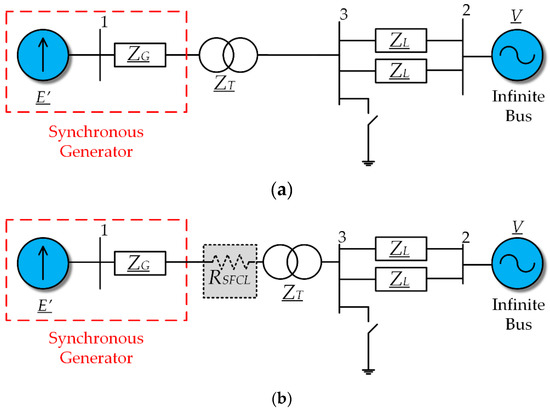
Figure 1.
Single machine infinite bus (SMIB) system for theoretical analysis: (a) without superconducting fault current limiter (SFCL) resistance; (b) with SFCL resistance.
The system parameters are given in Table 1. In this system, the synchronous generator power is delivered to the infinite bus via two transmission lines whose impedance is ZL. The generator is connected to the transmission system via a transformer whose impedance is ZT. The impedance (ZG) represents the generator transient impedance used in the transient stability analysis. E′ and V are the generator internal voltage and the infinite bus voltage, respectively.

Table 1.
System parameters for theoretical analysis.
The system is subjected to a three-phase ground fault on the transformer bus. The system transient stability without the extra resistance is evaluated using the EAC. For this, the swing equation is given in Equation (1), and the system power-angle relation in Equation (2) [1]:
where is the electrical power transmitted between bus 1 and 2, is the mechanical power in the generator shaft, is the generator rotor angle, is the angular speed, is the inertia constant, is the damping coefficient, is the system admittance matrix, is the first-row and first-column complex term of matrix , is the first-row and second-column complex term of matrix , and is the angle of the complex term .
The admittance matrix for the pre-fault and post-fault system is calculated using Equation (3), and is used in conjunction with Equation (2) to plot the power-angle curve for the pre-fault system in the EAC analysis:
During the fault, the generator electrical power becomes zero due to fault position and characteristic. After the fault clearing, the system topology is not altered and, therefore, the post-fault power-angle curve is the same for the pre-fault system. For this system configuration, the initial δ angle is equal to 0.6467 rad, while the CCA found using EAC is equal to 1.255 rad.
The proposed adaptation for the armature resistance works by adding an extra resistance in the virtual armature circuit of the VSG, as indicated in Figure 1b. In this scenario, for the pre-fault and post-fault systems, there is no extra resistance added. Therefore, the system admittance matrix is the same as in Equation (3). In contrast, during the fault occurrence, the extra resistance cannot be neglected and is considered in the calculation of the admittance matrix. The power-angle equation for the system during the fault is given by Equation (4) when considering this extra resistance [4]:
where e are the imaginary parts of the generator and transformer impedances.
Due to the presence of a three-phase fault in the transformer bus, the admittance between buses 1 and 2 (Y12) is nulled, and the second term of Equation (2) is zero. Consequently, the power-angle equation is dependent only on the real part of Y11, which in turn can no longer be neglected due to the presence of the SFCL resistance. Figure 2 shows the modification of the power-angle curves for different values of SFCL resistance.
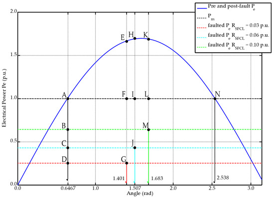
Figure 2.
Equal-area criterion with the operation of different values of RSFCL.
The acceleration areas for CCT in Figure 2 are defined by the areas between points ADGF (for = 0.03 p.u.), ACJI (for = 0.06 p.u.), and ABML (for = 0.10 p.u.). The deceleration areas are defined by the areas between points FEN (for = 0.03 p.u.), IHN (for = 0.06 p.u.), and LKN (for = 0.10 p.u.). In Figure 2, it is possible to observe that, with an increase in the resistance added during the fault, there is a gradual decrease in the acceleration area as the machine shaft acceleration is dampened. The added resistance is responsible for partially absorbing the extra energy injected in the generator shaft during the fault. Consequently, the machine rotor acceleration is dampened, and an increase in the CCA occurs. With the increase in CCA, the system remains in synchronism for a longer time, increasing its stability margin. Figure 3 illustrates this behavior, showing the evolution of CCA for different resistance values (from 0.0 p.u. to 0.16 p.u.).
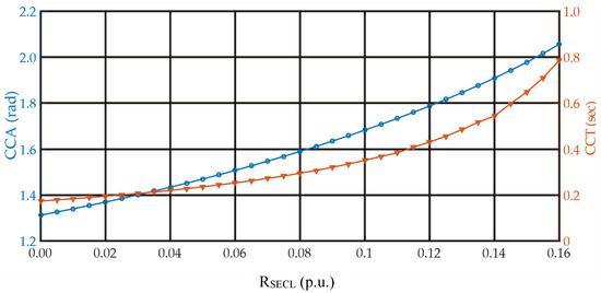
Figure 3.
Theoretical critical clearing angle (CCA) and critical clearing time (CCT) for different values of RSFCL.
The value of 0.16 p.u. is adopted as a limit because, at this point, the acceleration area A1 in the equal-area criterion is null, and CCA value equals the maximum angle for stability at 2.538 rad. The CCT is determined using the numerical solution of Equation (1), applying the fourth-order Runge–Kutta method. Figure 3 also shows the growth of CCT with the increasing SFCL resistance. It is possible to observe an improvement in system stability margin with the increase in , as observed for the CCA. For example, through the graph shown in Figure 3, the potential for increasing the CCT can be observed, since for an SFCL impedance of 0.1 p.u., a 100% increase in CCT is verified.
3. Proposed Adaptive Control and System Description
In this section, a modification in the VSG control loops to include the adaptive armature resistance characteristic will be discussed. The synchronous machine model used in the VSG will be presented along with the power converter used. Then, this section will present the system used to validate the theoretical stability analysis discussed in the previous section. For this purpose, a HIL test-bench, with the VSG control embedded on a microcontroller platform, is used.
3.1. VSG Implementation with Adaptive Control
3.1.1. Machine Model Used in the VSG Control
Several VSG implementations can be found in the literature with different names and features, but the emulation of the inertial electromechanical characteristic of synchronous machines is common to every implementation. Therefore, the development of a VSG control naturally implicates the use of the machine’s swing equation, Equation (1), in the active power control loop of the converter. Moreover, for the emulation of the machine windings electromagnetic behavior, a proper model must be adopted. In this paper, a two-axis model with transient and sub transient dynamics will be used [24]. Equations (5)–(8) are used to model the flux behavior in the machine windings:
Then, the transient voltages E are used to calculate the reference VSG voltages in Equations (9) and (10):
The output electrical power needed in the swing Equation in (1) is determined by Equation (11):
In Equations (5)–(11), and are the synchronous reactances, and are the transient reactances, and are the sub transient reactances, and are the open-circuit transient time constants, and are the open-circuit sub transient time constants, the voltages represented by the letter E are the transient and sub transient machine voltages, is VSG electrical power output, is the armature resistance, and are the VSG currents, and and are the VSG terminal voltages. The suffixes d and q indicate the direct and quadrature axis, respectively.
Additional control loops are used to adjust the VSG response during start-up and synchronization before the fault occurs to keep it running in steady-state. A loop to regulate the virtual machine excitation and its voltage is used, while a second loop performs angular speed and frequency regulation. Equation (12) is adopted to serve as the speed governor loop in this paper [25]:
where is the VSG active power setpoint, is the system nominal frequency in Hz, represents the VSG angular speed in p.u., and is the frequency droop gain.
The automatic voltage regulator (AVR) used is based on the DC1A excitation system defined in [26]. However, a simplified version is used by neglecting the over-excitation and under-excitation protections along with the exciter saturation effects. As a result, the system is comprised of a voltage regulator loop, a stabilization feedback loop, and the exciter model. The AVR used is shown in Figure 4, where and are the voltage regulator time constant and gain, and are the voltage regulator saturation limits, is the VSG voltage setpoint, is the VSG measured terminal voltage, and and are the feedback loop time constant and gain. The exciter is represented by a first-order loop, where and represents its time constant and gain. When the fault is applied to the system, these regulation loops are removed, so that the CCT found is dependent only on the machine’s inertia constant and the adaptive control applied.
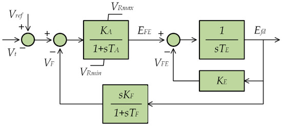
Figure 4.
Modified IEEE DC1A excitation system used as automatic voltage regulator (AVR) in the Virtual Synchronous Generator (VSG) control.
3.1.2. Proposed Adaptive Control Strategy
As seen in the previous section, this resistance added in series with the stator of synchronous generators can increase the system transient stability margin. Therefore, the armature resistance used to calculate the VSG terminal voltages in Equations (9) and (10) will follow Equation (13):
where is the original steady-state VSG armature resistance, and is the virtual SFCL resistance added when a fault occurs.
In the moments before and after a fault in the system, will be small to maintain the VSG operating in steady-state. The resistance value is raised to ( + ) during the occurrence of the fault. A fault detection algorithm is derived to allow the adaptive control to know the correct time to perform the resistance change. For this purpose, a simple scheme is proposed, in which the voltage dip during the fault is used as a pattern for detection. A voltage threshold is used so that when the fault is applied and the voltage magnitude drops below this value, the adaptive control changes the virtual resistance in the VSG adaptative resistance control. The resistance returns to its normal operation value when the voltage magnitude rises above this threshold. Figure 5 shows the complete adopted VSG diagram, with the speed and AVR regulators combined with the machine model with the proposed adaptive control.
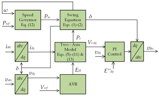
Figure 5.
Proposed VSG control diagram.
In Figure 5, represents the VSG output phase currents, and represents the VSG output voltages measured after the LCL filter. These measurements are transformed using the Park transformation, with the internal machine angle as the angular reference. The output of the calculated terminal voltages and are fed into a proportional-integral control loop (PI) to adjust the VSG output voltage. A positive feedback is implemented after the PI control loop using the transient voltages . The result is then fed to an inverse Park transformation to generate the converter switching references.
3.2. System Description for HIL Validation
In order to validate the theoretical analysis previously presented, a real-time simulation test-bench is proposed in a HIL environment. This technique involves simulating part of the system in real-time while another part remains an original part of the system. The VSG power electronics converter and the SMIB power system are simulated in real time in the Typhoon HIL environment, while the converter controller is implemented in the dSPACE microcontroller, the same way as in a real application. This type of HIL implementation is usually called control Hardware-in-the-loop (C-HIL) [27]. In this paper, the power system is simulated in real-time by the HIL module, as indicated in the red box in Figure 6. In the meantime, the VSG control strategy, including the proposed adaptation, will be embedded on a micro-controlled platform, indicated by the blue box in Figure 6.
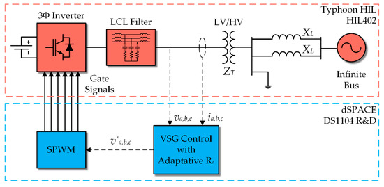
Figure 6.
Hardware in the loop (HIL) test-bench schematic.
The parameters used in the simulations are the same already defined in Table 1, with the addition of parameters shown in Table 2. The power system consists of a two-level, three-phase inverter with an LCL output filter, along with a transmission system consisting of a transformer, transmission lines and an infinite bus. The switching technique used to generate the converter gate signals is the Sinusoidal Pulse Width Modulated (SPWM).
Table 2.
VSG and power system parameters for HIL test-bench.
A Typhoon HIL 402 module is responsible for the real-time simulation of the power system part of the test-bench. Meanwhile, VSG control is calculated on a dSPACE DS1104 R&D controller. The power system variables, such as voltages and currents at the VSG point of connection, are extracted and sent to the dSPACE controller, through the analog outputs of the HIL 402, to the ADC inputs of DS1104. The DS1104 platform calculates the VSG model, and the pulse width modulation (PWM) signals are sent to the digital inputs of the HIL 402. The signals interface between HIL402 and DS1104 controller is accomplished by a breakout board, which distributes the HIL402 input and output signals into snap-in connectors for easy access. Figure 7 illustrates the connection diagram between the DS1104 and the HIL 402. Figure 8 shows the test-bench used.
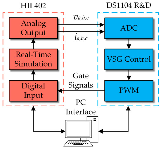
Figure 7.
The interface between the real-time simulation module HIL 402 and control platform dSPACE DS1104.
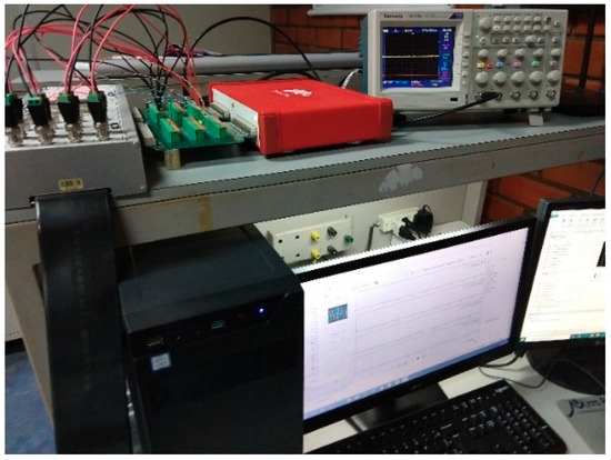
Figure 8.
Test-bench used to validate the adaptive control proposed.
The test-bench supervision and the results acquisition are done through the supervisory control and data acquisition (SCADA) platform provided by both HIL402 and DS1104 software packages. A trigger signal is generated in the real-time simulator environment to synchronize the data logging of system variables, for future analysis and use in the manuscript results Section 4. After the data acquisition, the results were plotted in graphs using the MATLAB software. Finally, oscilloscope curves were obtained from the power part, simulated in real time through the BNC connectors present in the HIL breakout board.
4. Results and Discussion
The system proposed in the previous section was simulated in a HIL environment, in order to verify the results found in the theoretical analysis made in Section 2. Thus, the HIL test-bench goal is to check if an increase in simulated CCT follows the adoption of the proposed adaptive control, thus proving its contribution to enhancing the system transient stability. Ergo, as proposed in the theoretical analysis, the CCT of the HIL test bench is checked for different values. The system is simulated for values ranging from 0.0 p.u. to 0.16 p.u., with a step of 0.01 p.u. For each value simulated, the CCT is found through repeated simulations in HIL, adjusting the fault time until the maximum fault time in which the system maintains synchronism. In order to shorten the process of finding the CCT, the theoretical CCT found is used as a starting point, and the bisection method is adopted with an accuracy of 1 ms. Altogether, 10 real-time simulations were performed on average to find the CCT in each scenario, which represents an average of 170 simulations performed for all scenarios. Simulation results were obtained using PSCAD software, to validate the theoretical analysis and to compare with the C-HIL results. The PSCAD simulates both power electronics and the proposed control strategy, while C-HIL has the control embedded in a microcontroller platform. By using an external digital controller, the C-HIL presents a gain in fidelity in relation to the purely simulated approach. The results for the system CCT with the adaptive VSG control is shown in Figure 9.
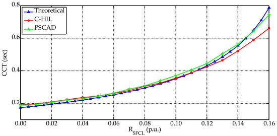
Figure 9.
Theoretical CCT (blue), PSCAD simulation (green) and C-HIL (red).
A detailed comparison between C-HIL and theoretical CCT is presented in Table 3, showing the CCT relative error for individual scenarios and the root mean square error (RMSE) considering all scenarios.
Table 3.
Relative error and root mean square error (RMSE) between C-HIL, PSCAD simulated and theoretical results.
The results revealed an increase in CCT when increasing the virtual resistance added. In particular, it is possible to observe an increase of 470 ms between the CCT for the highest value of , in real time C-HIL and the VSG, without changing the armature resistance in its model. This event represents a 346% increase in CCT and, therefore, in the power system stability margin. So, the results obtained through the real-time C-HIL corroborate the theoretical and PSCAD simulations analysis carried out, showing a consistent increase in the CCT with the increase in . The curves shown in Figure 9 reveal the same shape across the entire range of . A deviation between theoretical and simulated results (C-HIL and PSCAD) is observed, beginning at = 0.10 p.u. This could be explained mainly by the fact that, in the theoretical analysis, a simplified model of the machine is used to numerically determine the critical clearing angle and time. The machine model used in the VSG implementation is a high order model that includes both the swing equation and the machine winding modelling. The lack of fidelity in the model used in the theoretical analysis becomes noticeable when near the system stability boundary. However, the relative errors shown in Table 3 indicate a bounded error along the entire range of values, reaching a maximum of 16% at the limit. Further, the small RMSE calculated confirms the proximity between theoretical, PSCAD simulation and HIL CCT curves. Hence, the present results demonstrate that, although a real SFCL is not present in the system, its virtualized behavior in the VSG causes the contribution to the transient stability enhancement to be included in the system operation.
Similar results concerning the increase of CCT could be obtained for an adaptation of the inertia constant. Using the CCT as a figure of merit (FOM), a comparison between both parameter adaptation methods can be presented. Figure 10 shows the theoretical CCT for an inertia constant variation between 1.0 p.u. and 20.0 p.u., while not adding any extra resistance in the VSG armature circuit. The CCA does not change, because the inertia variation does not affect the system power-angle curves. Nonetheless, the change in inertia implicates in the swing equation resolution, leading to slower dynamics and a reduced machine acceleration during a fault, therefore increasing CCT. However, as discussed in the Introduction Section 1, the relation of CCT and inertia has a saturation characteristic, which eventually leads to diminishing returns in CCT with the rise in the inertia constant value. This saturation characteristics is shown in Figure 10, beginning at around = 10.0 p.u. From this point, an increase in inertia leads to diminishing returns in CCT, which leads to a maximum practical CCT between 300 ms and 400 ms. Meanwhile, the maximum theoretical CCT achieved by the proposed resistance adaptive control is 787 ms. Therefore, this result shows an advantage of the control strategy proposed in this paper due to its wider range of CCT.
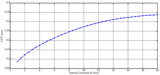
Figure 10.
Theoretical CCT for multiple values of inertia constant and = 0.0 p.u.
The VSG behavior for angular speed and rotor angle can be analyzed to confirm the improvement in stability. For this analysis, the fault clearing time is kept constant at 250 ms, and the system is simulated in real-time for different values. Figure 11 shows the rotor angular speed for the VSG in this situation, while Figure 12 shows the behavior of the rotor angle. The fault is applied in 0.5 s and extinguished at 0.75 s.
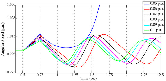
Figure 11.
Angular speed for a fault clearing time of 250 ms and different values of
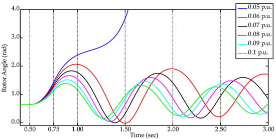
Figure 12.
Rotor angle for a fault clearing time of 250 ms and different values of
From the curve in Figure 11, it is possible to observe that the higher the resistance added into the VSG model during the fault, the lower the maximum speed reached by the machine at the fault clearing time. The acceleration of the VSG virtual rotor is not as steep in scenarios where adaptive control acts by increasing the resistance parameter. In other words, the extra energy injected into the machine’s rotor in the short-circuit is reduced. This result serves to corroborate the increase in CCT shown in Figure 9, proving the contribution of the proposed control to the system transient stability enhancement. Figure 11 demonstrates the increment of CCA with the increase of found through the EAC. The rotor acceleration is reduced, and the angular displacement is lower at the end of the fault. As a result, the system can reach higher levels of angular separation without hitting the critical energy absorption point. Figure 12 also shows that, for a higher resistance added by the adaptive control, more restrained are the angular oscillations, which is reflected in a dampened active power response after the fault clearance. This drives the system to lower settling times for the post-fault VSG dynamic response. It is worth noting that the base for the angular speed, represented in Figure 11, is defined by the system nominal frequency in radians per second, in this case 376.99 rad/s. The initial value of rotor angle, shown in Figure 12, is related to the initial machine angle for steady state, calculated in Section 2 by the EAC as 0.6467 rad.
Additionally, the phase plane shown in Figure 13 can be used to condense the results exhibited in Figure 11 and Figure 12. A phase plane is a graphical tool that allows visualization of the system trajectory in fault situations. In cases where the system remains stable after the fault is cleared, it is possible to observe in Figure 13 that the system trajectory remains bounded and moves towards a new equilibrium point. The trajectory is more restrained at both speed and angle axis for higher values of resistance. However, when the system loses synchronism after the fault ( = 0.05 p.u., for example), the trajectory of the system exits the stability region on an infinite movement. The phase plane is commonly compared to a sphere inside a bowl problem [1]. An injection of energy in the ball starts its movement towards the bowl edge. When the energy injected is sufficient to make the sphere drop out of the bowl, the system is called unstable.
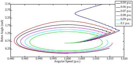
Figure 13.
Phase plane representation for a fault clearing time of 250 ms and different values of .
The parallel could be made to the power system stability by defining the sphere as the generator or the VSG, and the bowl is represented in a two-dimensional system by the rotor speed and angle, like the phase plane. When sufficient energy is added to the generator axis, the system is not able to absorb it, and the generator trajectory represented in the phase plane escapes from the bounded stability region. In the case regarding the adaptive control proposed, the extra virtual resistance is capable of absorbing part of the energy injected in the VSG virtual rotor, restricting its movement inside the stability region.
Figure 14 and Figure 15 are used to show the system voltage behavior on the transformer low voltage (LV) side, in pre-fault, during-fault and post-fault instants. Figure 14 shows the system line voltage for a 250 ms fault and = 0.0 p.u. Figure 15 shows two scenarios for non-zero values. Figure 15a presents a scenario in which the system remains stable for = 0.06 p.u., while Figure 15b shows the stable system for = 0.1 p.u.
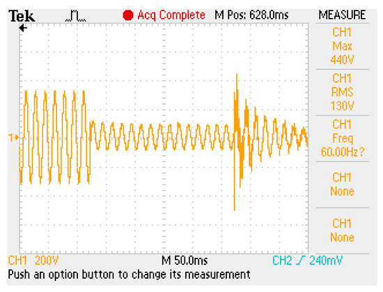
Figure 14.
VSG output voltage for a 250 ms short-circuit and = 0.0 p.u.
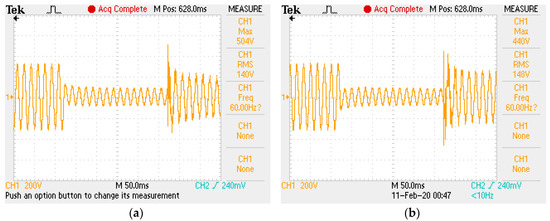
Figure 15.
VSG output voltage for a 250 ms short-circuit: (a) with = 0.06 p.u.; (b) with = 0.1 p.u.
It can be observed in Figure 14 that the voltage collapses shortly after the end of the fault, indicating the system instability for these conditions. For the C-HIL scenario shown in Figure 14, where = 0.0 p.u., the CCT defining the stability limit is 191 ms, as presented in Table 3. In contrast, Figure 15a,b show a disposition for the VSG voltage to return to nominal values. In particular, for the situation in Figure 15b where = 0.1 p.u., the VSG voltage after the fault has a faster settling time, and returns more quickly to a steady-state level. Moreover, the maximum voltage overshoot reached at the time of fault clearance for = 0.1 p.u. is lower compared to the VSG with = 0.06 p.u. In the first case, the voltage reaches 504 V when the fault is cleared, while for the second scenario the voltage reaches a maximum of 440 V. Both C-HIL scenarios in Figure 15 presented post-fault stability, due to their higher CCTs provided by the adaptive control. For the scenario in Figure 15a, the stability boundary is defined by a CCT of 261 ms. Meanwhile, the scenario shown by Figure 15b has a stability boundary defined by a CCT of 355 ms. Both results are shown in Table 3.
Eventually, if a control strategy such as the one proposed in this paper is implemented in a real power system, its interaction with the system protection devices must be carefully addressed. For example, the actuation time of overcurrent relays used to remove a faulted line, which usually consider the CCT for their coordination, must now be aware of the proposed control dynamics. The operation of out-of-step protection functions and distance relays are also of special importance when dealing with transient improving control strategies. On the other hand, an adaptive control that improves CCT in a power system could be used in a preventive scheme, to maintain the fault critical time in a fixed value for different generator loading levels, and system topology during the day.
5. Conclusions
This paper presents a new adaptive control strategy for the control of VSG-based power converters. An alteration in the synchronous machine model used in the VSG implementation is made in order to incorporate the behavior of resistive SFCL in short-circuit situations. With this, the VSG’s armature resistance parameter is modified to virtualize the SFCL dynamics. The objective is to show that SFCL virtualization through the proposed adaptive control can improve the transient stability of power systems with connected VSGs. A theoretical analysis is carried out, and the results are verified through real-time simulation in a Hardware-in-the-loop environment.
The results show an increase in the system CCT with the proposed adaptive control for all RSFCL values. Additionally, the results show that the increase in the CCT accompanies the increase in the RSFCL values, showing a characteristic of direct proportionality. The C-HIL results show compliance with the theoretical result, with both CCTs showing similar values with limited relative errors and RMSE. The analysis based on the EAC is corroborated by the results of angular speed and rotor angle, that point to damping in the VSG acceleration during the fault. The VSG voltages show the difference between instability and stability scenarios. It is possible to conclude that the adaptive control can improve the voltage response of the VSG at the end of the fault, by increasing the system transient stability margin.
The increase in CCT demonstrates the improvement in the system transient stability margin and, since this is achieved by virtualizing the behavior of a physical device, the proposed adaptive control shows that it can contribute to improving the stability of the system without the need to change its topology.
Author Contributions
Conceptualization, D.C., A.E.A.A. and L.F.E.; Formal analysis, D.C.; Funding acquisition, L.F.E.; Methodology, D.C., A.E.A.A. and L.F.E.; Project administration, L.F.E.; Software, D.C. and T.S.A.; Supervision, D.S.L.S. and J.F.F.; Validation, D.C. and T.S.A.; Visualization, D.C.; Writing—original draft, D.C. and T.S.A.; Writing—review & editing, A.E.A.A., T.S.A., D.S.L.S., J.F.F. and L.F.E. All authors have read and agreed to the published version of the manuscript.
Funding
This study was financed in part by the Coordenação de Aperfeiçoamento de Pessoal de Nível Superior—Brasil (CAPES)—Finance Code 001, Fundação de Amparo à Pesquisa e Inovação do Espírito Santo—Finance Codes 117/2019 and 536/2018. The APC was funded by Fundação de Amparo à Pesquisa e Inovação do Espírito Santo.
Acknowledgments
The authors acknowledge the support given by Typhoon HIL for the HIL 402 hardware platform that was donated in the “10 for 10 Typhoon HIL Awards Program”.
Conflicts of Interest
The authors declare no conflict of interest.
References
- Sauer, P.W.; Pai, M.A.; Chow, J.H. Power System Dynamics and Stability: With Synchrophasor Measurement and Power System Toolbox, 2nd ed.; John Wiley & Sons: Hoboken, NJ, USA, 2017. [Google Scholar]
- Safaei, A.; Zolfaghari, M.; Gilvanejad, M.; Gharehpetian, G.B. A survey on fault current limiters: Development and technical aspects. Int. J. Electr. Power Energy Syst. 2020, 118, 105729. [Google Scholar] [CrossRef]
- Lee, S.; Lee, C.; Ko, T.K.; Hyun, O. Stability analysis of a power system with superconducting fault current limiter installed. IEEE Trans. Appl. Supercond. 2001, 11, 2098–2101. [Google Scholar] [CrossRef]
- Almeida, M.E.; Rocha, C.S.; Dente, J.A.; Branco, P.J.C. Enhancement of power system transient stability and power quality using superconducting fault current limiters. In Proceedings of the 2009 International Conference on Power Engineering, Energy and Electrical Drives, Lisbon, Portugal, 18–20 March 2009; pp. 425–430. [Google Scholar] [CrossRef]
- Alaraifi, S.; El Moursi, M.S. Design considerations of superconducting fault current limiters for power system stability enhancement. IET Gener. Transm. Distrib. 2017, 11, 2155–2163. [Google Scholar] [CrossRef]
- Didier, G.; Leveque, J.; Rezzoug, A. A novel approach to determine the optimal location of SFCL in electric power grid to improve power system stability. IEEE Trans. Power Syst. 2013, 28, 978–984. [Google Scholar] [CrossRef]
- Son, G.T.; Lee, H.J.; Lee, S.Y.; Park, J.W. A study on the direct stability analysis of multi-machine power system with resistive SFCL. IEEE Trans. Appl. Supercond. 2012, 22. [Google Scholar] [CrossRef]
- Sung, B.C.; Park, D.K.; Park, J.; Ko, T.K. Study on a Series Resistive SFCL to Improve Power System Transient Stability: Modeling, Simulation, and Experimental Verification. IEEE Trans. Ind. Electron. 2009, 56, 2412–2419. [Google Scholar] [CrossRef]
- Peddakapu, K.; Mohamed, M.R.; Sulaiman, M.H.; Srinivasarao, P.; Reddy, S.R. Design and simulation of resistive type SFCL in multi-area power system for enhancing the transient stability. Phys. C Supercond. Appl. 2020, 1353643. [Google Scholar] [CrossRef]
- Didier, G.; Bonnard, C.H.; Lubin, T.; Lévêque, J. Comparison between inductive and resistive SFCL in terms of current limitation and power system transient stability. Electr. Power Syst. Res. 2015, 125, 150–158. [Google Scholar] [CrossRef]
- Alshahrani, A.; Omer, S.; Su, Y.; Mohamed, E.; Alotaibi, S. The Technical Challenges Facing the Integration of Small-Scale and Large-scale PV Systems into the Grid: A Critical Review. Electronics 2019, 8, 1443. [Google Scholar] [CrossRef]
- Shah, R.; Mithulananthan, N.; Bansal, R.C.; Ramachandaramurthy, V.K. A review of key power system stability challenges for large-scale PV integration. Renew. Sustain. Energy Rev. 2015, 41, 1423–1436. [Google Scholar] [CrossRef]
- Beck, H.-P.; Hesse, R. Virtual synchronous machine. In Proceedings of the 2007 9th International Conference on Electrical Power Quality and Utilisation, Barcelona, Spain, 9–11 October 2007; pp. 1–6. [Google Scholar] [CrossRef]
- Driesen, J.; Visscher, K. Virtual synchronous generators. In Proceedings of the 2008 IEEE Power and Energy Society General Meeting—Conversion and Delivery of Electrical Energy in the 21st Century, Pittsburgh, PA, USA, 20–24 July 2008; pp. 1–3. [Google Scholar] [CrossRef]
- Zhong, Q.-C.; Weiss, G. Static synchronous generators for distributed generation and renewable energy. In Proceedings of the 2009 IEEE/PES Power Systems Conference and Exposition, Seattle, WA, USA, 15–18 March 2009; pp. 1–6. [Google Scholar] [CrossRef]
- Encarnação, L.; Carletti, D.; Souza, S.; de Barros, O., Jr.; Broedel, D.; Rodrigues, P. Virtual Inertia for Power Converters Control. In Advances in Renewable Energies and Power Technologies. Volume 2, Biomass, Fuel Cells, Geothermal Energies, and Smart Grids; Yahyaoui, I., Ed.; Elsevier Science: Amsterdam, The Netherlands, 2018; pp. 377–411. [Google Scholar] [CrossRef]
- Li, M.; Huang, W.; Tai, N.; Yu, M. Lyapunov-Based Large Signal Stability Assessment for VSG Controlled Inverter-Interfaced Distributed Generators. Energies 2018, 11, 2273. [Google Scholar] [CrossRef]
- Alipoor, J.; Miura, Y.; Ise, T. Power System Stabilization Using Virtual Synchronous Generator with Alternating Moment of Inertia. IEEE J. Emerg. Sel. Top. Power Electron. 2015, 3, 451–458. [Google Scholar] [CrossRef]
- Li, J.; Wen, B.; Wang, H. Adaptive virtual inertia control strategy of VSG for micro-grid based on improved bang-bang control strategy. IEEE Access 2019, 7, 39509–39514. [Google Scholar] [CrossRef]
- Li, D.; Zhu, Q.; Lin, S.; Bian, X.Y. A Self-Adaptive Inertia and Damping Combination Control of VSG to Support Frequency Stability. IEEE Trans. Energy Convers. 2017, 32, 397–398. [Google Scholar] [CrossRef]
- Torres L., M.A.; Lopes, L.A.; Moran T., L.A.; Espinoza C., J.R. Self-Tuning Virtual Synchronous Machine: A Control Strategy for Energy Storage Systems to Support Dynamic Frequency Control. IEEE Trans. Energy Convers. 2014, 29, 833–840. [Google Scholar] [CrossRef]
- Li, M.; Huang, W.; Tai, N.; Yang, L.; Duan, D.; Ma, Z. A Dual-Adaptivity Inertia Control Strategy for Virtual Synchronous Generator. IEEE Trans. Power Syst. 2019, 35, 594–604. [Google Scholar] [CrossRef]
- Kerdphol, T.; Watanabe, M.; Hongesombut, K.; Mitani, Y. Self-Adaptive Virtual Inertia Control-Based Fuzzy Logic to Improve Frequency Stability of Microgrid with High Renewable Penetration. IEEE Access 2019, 7, 76071–76083. [Google Scholar] [CrossRef]
- Machowski, J.; Bialek, J.W.; Bumby, J.R. Power System Dynamics: Stability and Control, 2nd ed.; John Wiley & Sons: West Sussex, UK, 2008. [Google Scholar]
- Zhang, C.H.; Zhong, Q.C.; Meng, J.S.; Chen, X.; Huang, Q.; Chen, S.H.; Lv, Z.P. An Improved Synchronverter Model and its Dynamic Behaviour Comparison with Synchronous Generator. In Proceedings of the 2nd IET Renewable Power Generation Conference (RPG 2013), Beijing, China, 9–11 September 2013; Institution of Engineering and Technology: London, UK, 2013; pp. 4–13. [Google Scholar] [CrossRef]
- IEEE Power and Energy Society. IEEE Recommended Practice for Excitation System Models for Power System Stability Studies; IEEE: Piscataway, NJ, USA, 2016. [Google Scholar] [CrossRef]
- Genic, A.; Gartner, P.; Almeida, M.; Zuber, D. Hardware in the Loop Testing of Shipboard Power System’s Management, Control and Protection. In Proceedings of the 2017 IEEE Vehicle Power and Propulsion Conference, VPPC 2017—Proceedings, Belfort, France, 11–14 December 2017; Institute of Electrical and Electronics Engineers Inc.: Piscataway, NJ, USA, 2018; pp. 1–6. [Google Scholar] [CrossRef]
© 2020 by the authors. Licensee MDPI, Basel, Switzerland. This article is an open access article distributed under the terms and conditions of the Creative Commons Attribution (CC BY) license (http://creativecommons.org/licenses/by/4.0/).