Abstract
A bi-level electricity market clearing process was developed for energy and reserve allocation in the day-ahead market using AC Optimal Power Flow (ACOPF). An energy-consuming entity (ECE) which does not want its cleared demand to be curtailed, even if any contingency occurs, purchases power from the reserve market at a higher rate. The proposed model helps the ECE to secure a reserve market allocation at the price of the energy market in the real-time market settlement. Various market models were formulated for the evaluation of locational marginal pricing (LMP) in the energy market and locational contingency marginal reserve pricing (LCMRP) in the reserve market. The impact of wind farms on LMP, LCMRP, and negative LMP was analyzed. The increase in demand requirement in the deregulated environment was balanced in the proposed models by the thermal–wind coordination dispatch. The market models were illustrated with the IEEE 30 bus system.
1. Introduction
The deregulated electric industry, in reality, approaches higher economic efficiency and lower electricity prices. The restructured power system network has the balance to supply demand from flexible coal generators and partially unpredictable renewable energy sources. In contemporary renewable energy, the spinning and non-spinning reserves meet unexpected rises in demand. This milieu enforces the optimal scheduling of all generations. The levy paid for an MW increase in demand at a node, decided by the independent system operator (ISO), depends on the source of supply, which defines the locational marginal pricing (LMP) or the nodal pricing. The penetration pricing of renewable energy is set low to reach a wide fraction of the electricity market, which redefines thermal generation as the flexible generation, and also plays a vital role in the assessment of LMP.
There are various approaches to determining LMP, considering the transmission, contingency, reserve constraints, etc., which meet reliability and security in a system, i.e., with optimal generation unit dispatch. In 1988, F.C.Schweppe introduced the term locational marginal pricing [1]. The concept of LMP has been implemented by many ISOs, for example, PJM, New York ISO, CAISO, ISO—New England, and Midwest ISO. LMP, being the by-product of OptimalPower Flow (OPF), can be solved by either DCOPF or ACOPF. DCOPF analysis gives an exact value of energy cost, which can be further analyzed for congestion cost and loss cost, whereas ACOPF gives a levy, which requires a unique decomposition of costs. A systematic DCOPF approach presents a wide view of congestion and price vs. load, i.e., the price at a node with uncertainty in the load [2]. Load uncertainty leads to volatility in LMP, which is described as LMP uncertainty in the probabilistic sense [3]. This LMP fluctuation requires a price risk hedging instrument, which involves the correct decomposition of loss and congestion components, which are very critical for the calculation and settlement of these financial questions. The developed LMP decomposition algorithm overcomes the dependence on the choice of the slack bus [4,5].
The load-serving entity (LSE) and energy-consuming entity (ECE) work for their own maximum profit by bidding on the selling and purchase price. Maximizing the profit or minimizing the fuel cost becomes the objective function in clearing the electricity market, subjected to various constraints. The objective function decides the optimal dispatch of generators. On the other side, by assessment of the size and location of distributed generators (DGs), the LMP can be minimized. The DGs contribute to more advantages, including environmental, economic, and technical.
Wind power is the emerging renewable energy-generation resource in many countries [6]. With increasing oil and gas prices and growing global energy demand, wind power has strong potential for future power generation. Wind power generation is an attractive auxiliary to turbulent fossil fuel prices in the global environment, because of its fuel-free and emission-free nature [7]. The main issue with wind power is its unpredictability and uncertainty. Unpredictability means the inability to predict wind power accurately, which leads to variations in power balance. Wind speed varies with the seasons and the time of the day, and wind generation strongly depends on wind speed.
In countries like North America, wind power is scheduled either in the day-ahead market or the real-time market, because of its uncertainty [8]. In such cases, a sufficient quantity of reserve is also maintained in operational planning. This reserve requirement can be calculated by the probability distribution function (PDF) of wind power generation. The wind speed profile is developed by a known PDF and transformed into corresponding wind power distribution. A review of wind speed probability distribution was done in Reference [9]. An economic load dispatch model was developed in Reference [10], considering wind and thermal generators with the probability of stochastic wind power generation as a constraint. Additionally, the study included a factor for the overestimation and underestimation of wind power in an optimal power flow model, along with an objective function, i.e., fuel cost minimization. Rather than forecasting the wind and enforcing a penalty for overestimation and underestimation, this paper ensured the maximum scheduling of available wind power for energy, as well as the reserve market. The high penetration and large scale integration of wind farms have reduced the role of thermal generators, but wind cannot compensate for fast-acting generators, because of its volatility. A novel approach was presented in Reference [11], with two-stage robust energy and reserve scheduling taking into account wind generation uncertainty.
The key point is that wind energy is variable and intermittent. This variable nature of wind energy has been discussed in Reference [12]. Even during severe storms, the turbines need several hours to shut down—they will not disconnect altogether. Additionally, the failure of a turbine does not affect the system, as they are modular and diffused. Wind speed is predictable and wind power generation has been forecasted within a reasonable margin of error. Here, optimal power flow modeling has been done to utilize wind power in the energy market, and also in the reserve market. The incorporation of renewable energy is a challenging problem, and its uncertainty is addressed in Reference [13], in which the author proposed a novel optimal scheduling strategy for hybrid renewable generation systems.
The operating reserve includes the spinning and the non-spinning reserve. The spinning reserve (SR) is the vital supplementary service used to maintain system reliability if any unforeseen events occur, e.g., generator outages, line outages, and generation changes. Spinning reserve procurement has a significant bearing on economic dispatch and unit commitment; hence, it is kept at a minimum. The units generated for SR are therefore adjusted to maintain minimum operating costs [14]. Transmission line contingency with a high penetration of renewables has been discussed in Reference [15]. If the same generators contribute to the energy and reserve markets, then this provides more secure economic solutions. The non-spinning reserve is also defined as readily available generating capacity, but with a short time delay.
North American Electric Reliability Corporation (NERC) defines contingency reserve (CR) as all the committed reserves that can take up the demand in the required time. In deregulated power systems, CR has been taken into account in operational reliability analysis. Even PJM and CAISO include CR in their system operation process. Customer participation becomes a key issue in contingency reserve allocation. Based on customer requirements, they bid for quantity as well as the price they are willing to pay. Some need uninterrupted energy supply even during a contingency and are not bothered about the price, whereas some will be interrupted, because of the high contingency reserve cost and their unwillingness to pay this high cost. The LSEs and ECEs bid every hour in the market to supply and purchase energy, along with their bid price and quantity, and the ISO schedules the energy and reserve MW quantity. This joint clearing has been analyzed in many articles to determine the LMP of energy and reserve. Since there is a single power balance equation at a node, there can be only one price, but the reserve price charged cannot be the same as the energy price. Abetter strategy has to be implemented to ameliorate the negative effects of the deregulated energy market. Some ECEs dislike curtailment and thus put forth a bilateral contract with the LSE stating their willingness to pay and the quantity to be supplied even at times of contingency. The energy market clearing and settlement when the ECE also submits a bid to the ISO was presented in Reference [16] using the distributed slack bus concept, which reduces the burden of supplying loss by a single slack bus. Settlement and optimal pricing in restructured power systems have been analyzed in recent studies using various artificial intelligence techniques.
This paper presents an optimal power flow model for optimal MW generation scheduling and MW reserve scheduling of thermal generators and wind generators. With low wind penetration, wind generation acts a negative load, i.e., scheduling is of thermal generators alone. In such cases, all wind power is to be consumed and the levy given by the ISO must be accepted. Here, wind power is considered only dispatchable, i.e., not schedulable. This is to increase the allocation of wind generation. With an increase in wind penetration, wind generation can also be scheduled, and thus can bid in the market. However, a considerable amount of reserve must be allocated. If bids are accepted, the contracted power has to be delivered, if not, penalties are imposed. To avoid penalties, better forecasting tools and techniques are used by wind farms. However, wind farms are allowed to bid only in the day-ahead electricity market. At times, depending on availability, they enter into the real-time market. The ISO is also responsible for clearing the energy and the reserve market, after obtaining the bid price and bid quantity from the LSEs and ECEs.
This paper presents an optimal power flow model with elastic and inelastic demand for the assessment of locational marginal pricing and locational contingency marginal reserve pricing (LCMRP). The model also includes the high penetration of wind generation as both schedulable and non-schedulable. Additionally, a modified optimal power flow model for the unique pricing of the operating reserve and energy has been developed. Considering the zero fuel cost of wind and accurate forecasting of wind generation in the day-ahead market, the wind farm is allowed to participate in the energy market and also as CR in the operating reserves market, in such a way that maximum wind power is used, subject to operating conditions. That is, wind generators behave similarly to conventional generators, with the main difference that the maximum wind generation depends on wind availability at that hour. Except for the above, wind generators are less constrained than conventional thermal generators, i.e., no minimum generation limits, no minimum up times, usually high ramp rates. To conclude, wind generators are allowed to participate as flexible generators in energy and reserve markets. Herein, we bridge the gap of using wind farm generation for the energy market alone. However, there is a difference between the scheduling of generators in the real-time market and the day-ahead market; hence, a better bidding strategy should be adopted for true optimal scheduling of generators [17,18].
2. Problem Formulation
The LSE participates in the market by submitting a bid to the ISO. The ISO allocates a sufficient quantity of MW for reserves. Countries like Spain have large wind farms. The wind farms are allowed to bid on the day-ahead market, similar to the thermal generators. Thus, there exists a fair competition. If the bid is accepted, the contracted quantity is to be delivered by the wind farm.
This paper aimed to develop a bi-level electricity market clearance, in which the energy market is cleared by the ISO in Step 1, followed by reserve market clearance in Step 2. Various market models have been developed for clearing the energy market. Market Model 1 considers only the thermal generators as schedulable LSEs. Model 2 includes all features of Model 1; in addition, the fit-and-forget windfarms at the buses are considered as negative loads. Market Model 3 includes the thermal generators and wind farms as schedulable LSEs. Following the energy market clearance through Market Models 1, 2, and 3, the reserve market is cleared by Market Models 1r, 2r, and 3r respectively.
2.1. Step 1: Day-Ahead Energy Market Clearing
The day-ahead energy market clearing market models are as follows:
2.1.1. Market Model 1: Inelastic Demand Without Wind Penetration
The objective was the minimization of the total generation cost of satisfying the inelastic energy requirements of the energy-consuming entity. This model considered a day-ahead economic dispatch with optimal energy scheduling with various stability and reliability constraints; the optimization horizon was set as T = 24 with hourly steps. The inelastic demand redefined as a “single-sided auction” in the electricity market. The objective function was formulated as:
subjected to
The term in Equation (1a) is the quadratic fuel cost function of conventional thermal generator, which is given by , where , , and are fuel cost coefficients. Equations (1b) and (1c) represent the energy balance equation to supply the committed load for the normal state. The minimum and maximum generation limits include the ramp rate constraints given by Equations (1d) and (1e), beyond which it is not feasible to generate for techno-economic reasons. In Equation (1d), the LSE capacity was adjusted to account for reserve bidding. The generation limits were specified as the upper and lower limits for real and reactive power. The voltage magnitude limits and phase angle limits at the buses are given in Equations (1f)–(1g) respectively. Equation (1h) represents the transmission line flow limit, based on thermal considerations. The Lagrangian was formulated to solve the optimization problem, considering Equations (1a)–(1h). The Lagrangian multiplier of the real power balance constraint gave the marginal energy cost and thus the nodal price for the next MW of energy supplied at each node. In the normal state, the nodal price was given by $/MWh.
2.1.2. Market Model 2: Inelastic Demand with Fit-and-Forget Wind Penetration
In this market model, both the demand and the wind farm generation were inelastic. The wind farm real power generation was considered a negative load in the equality constraints and thus was only dispatchable, i.e., non-schedulable.
subjected to all constraints of Market Model 1, with modified real power equality constraints:
2.1.3. Market Model 3: Inelastic Demand with Wind Penetration Scheduling
In this market model, a linear bid was considered for the wind farms in the objective function, and part of the wind farm generation was allocated for contingency reserve. Here, the scheduling of generators was done for maximum utilization of the available wind generation in that particular hour. The wind power limits are determined by the grid operator, and the limits can be derived related to the reliability and security level of the system.
subjected to all constraints in Market Model 2, with minimum and maximum wind generation capacity as additional constraints:
The first term in Equation (3a) represents the quadratic fuel cost function of thermal generation, as given in Market Model 1, and the second term represents the direct cost given by the wind farm owner for specified wind power. A linear cost function used for wind power is given by .
The above Market Models 1, 2, and 3 represent the base optimal power flow model, imposing different scenarios. Once the energy market quantity and price are cleared by the ISO, the difference between the maximum MW limit and the energy market MW quantity becomes the maximum reserve allocation quantity. Clearing of energy MW quantity followed by reserve MW quantity is the design methodology of the Nordic market. The reserve energy procurement in the current electricity market is still done by ISO to maintain secure and economic operations, and also to maintain consistent reliability via a competitive bidding process. The LSE submits the bid and supply to the reserve market, so as to make more profit than the energy market with the available energy. The contingency reserve or operating reserve is essential only for the duration of the outage, and it is an option that can be called upon.
Normally, thermal generation is considered for the primary reserve, as it is the generation available at all times, with a specified maximum limit. Wind generation is used when available, but, because of its uncertainty, it cannot be considered for primary reserve. Nowadays, with accurate forecasting techniques and considering economic factors, wind farms can also participate in the primary OPF to balance demand, and the remnant can also participate in the secondary OPF to supply the contingency reserve. The wind farms now supply the ECEs more than a thermal generation.
Thus, revamping of the formulation of the market models was required to meet the demand requirement under contingency. Operating contingencies may or may not occur, but ECEs do not want their loads to be curtailed. Therefore, the ECEs also bid in the power market to get their reserve quantity and levy cleared in advance, based on the demand bid MW and price given by them, to be on the safe side in case of contingency.
Here, the sequential scheduling of generators was done for the day-ahead market. Primarily, OPF analysis was done so as to meet the dynamic variations of the ECE by the LSE, followed by the incremental OPF (IOPF) for contingency reserve scheduling, subjected to various techno-economical and reliability constraints. Below, to calculate the cost of the next MW required in the CR market, defined as locational contingency marginal reserve pricing (LCMRP), the above Market Models 1, 2, and 3 have been modified for IOPF into Market Models 1r, 2r, and 3r, respectively, with pricing for contingency reserve energy included in the objective function. The IOPF problem has been formulated to allocate the operating reserve from the available spinning reserve to supply the contingency demand requirements, so as to minimize the reserve energy cost.
2.2. Step 2: Day-Ahead Contingency Reserve Market Clearing
The day ahead reserve market scheduling market models are as follows:
2.2.1. Market Model 1r: Market Model 1 with Contingency Reserve Scheduling
This market model emphasized the delivery of the contingency reserve, with a linear cost function and auction only on thermal generation. The contingency reserve in this market model was supplied by flexible coal generators, alongside the scheduling of the above for the inelastic demand in Market Model 1. The already scheduled generations in Market Model 1 are specified by the superscript “0”. The incremental optimal power flow was formulated as:
subjected to
The Equations (1rb) and (1rc) represent the energy balance for supplying the inelastic demand in the normal state and in the contingency reserve state. Equation (1rd) is the thermal LSE’s output limit, considering the contingency reserve allocation. Equation (1rf) clinches each contingency reserve allocation within the limits of the up and down ramp rate, as well as bidding. Optimal CR allocation of every LSE to meet the contingency demand requirement can be determined by solving Equations (1ra)–(1ri). The Lagrangian function was formulated to solve the optimization problem. The Lagrangian multiplier of the energy balance constraint gave the marginal reserve energy cost, and thus the nodal reserve market price of supplying the next MW contingency demand at each node, which can be called the locational contingency marginal reserve pricing (LCMRP).
2.2.2. Market Model 2r: Market Model 2 with Contingency Reserve Scheduling
This model was formulated to supply the contingency demand requirement alongside the allocation of the inelastic demand in Market Model 2.
subjected to all constraints of Market Model 1r, with modified real power equality constraints as:
The above equation includes the LSE and wind farm scheduling from Market Model 2.
2.2.3. Market Model 3r: Market Model 3 with Contingency Reserve Scheduling
This model was formulated to supply the contingency demand requirement at minimal cost, alongside the allocation of demand by LSE and wind farms in Market Model 3.
subjected to constraints in Market Model 1r and Market Model 2r, with additional wind farm constraints:
3. Case Study
The modified IEEE 30 bus system was analyzed to compare the various market models. The different market models were formulated to determine the optimum dispatch of flexible coal generators and wind farms in the grid. The test system consisted of six generators at buses 1, 2, 5,8,11, and 13. The wind farms W1, W2, and W3 were assumed to be at buses 5, 15, and 25, respectively, and their hourly wind speed profile is given in Table A5. The wind speeds used were from Ottawa, Quebec, and Toronto weather stations, and the cut-in speeds were considered unique for each station. The maximum wind power generated [19] during each hour was determined based on the mathematical expression:
where are, respectively, cut-in and cut-out (furling) wind speeds, and is the rated wind speed at which the wind turbine rated output will be the rated output power .
The LSE cost coefficient profile and the branch profile of the modified IEEE 30 bus system are shown in Table A1 and Table A2, respectively. The cost coefficient profile of windfarm is shown in Table A3. The contingency reserve required was generally based on some heuristics such as the largest expected generation outage or a percentage of the expected demand, or both [20]. The linear bid was considered for the contingency reserve, which must supply the demand requirement without curtailment, and the demand requirement during contingency was 20% of the day-ahead load schedule. The contingency reserve was allocated within the maximum capacity of every LSE, and the maximum reserve quantity amounted to . Since the same generator can supply the energy and the contingency reserve, their reserve bid levy was 25% more than that of the energy bid. Thus, the pricing for nodal energy and reserve market at a node varied. The day-ahead load profile for every hour is shown in Table A4, and the load was shared across all nodes of the network.
The energy market and reserve market clearing and settlement for the proposed market models were illustrated using the IEEE 30 bus system in three steps.
- Analysis I: Energy and reserve schedules of the available LSEs were analyzed.
- Analysis II: Calculation of LMP in the energy market, which acts as a signal to the reserve market.
- Analysis III: Impact of wind penetration on negative LMP was analyzed.
3.1. Analysis I: Energy and Reserve Schedule of LSEs
Here, the contributions of the LSEs, i.e., the thermal and windfarm generators for the energy and reserve markets, to different models were analyzed. The optimal scheduling was done with the minimization of fuel cost as an objective function. As a result, a low-cost LSE will be cleared to the maximum quantity by the ISO, but the optimization has to balance the transmission line constraints.
Figure 1 gives the day-ahead energy schedule and reserve schedule in columns 1 and 2, respectively. Considering Market Model 1, the lowest levy generator Pg1, was scheduled the highest. The generator Pg5 contributed during the peak load period. Even though the costs of Pg1 and Pg2 were the same, Pg2 made less contribution. In Market Model2, the contribution of low-cost generators was reduced considerably compared to Market Model 1, as the wind farm generation at a node was solely devoured by the demand at that corresponding node. Market Model3 never incited the cost of thermal generators. In Market Model 3, the wind generators with pricing equal to that of low-levy generators became functional, and the OPF forced the maximum usage of available wind farm generation in that particular hour, which led to a major share of scheduling being granted to wind power. Additionally, the network constraints did not allow complete usage of the wind farm generation. Hence, the rock-bottom scheduling of thermal generators became imperative.
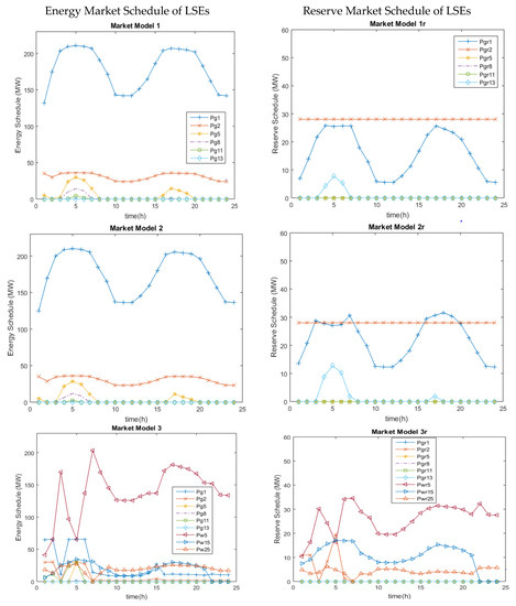
Figure 1.
Energy and reserve schedules of LSEs.
Considering the day-ahead reserve market schedule in Figure 1, since the low-levy LSEs filled the demand in the base case of the OPF market models, the remnant in each LSE was scheduled for the reserve market. Under such a scenario, the IOPF was forced to use the high-levy LSEs to meet the contingency demand requirement (CDR), as a result of which, the MW from the available low-levy LSEs, followed by the high-levy LSEs were scheduled in the reserve market. The highest contribution by Pg2 was in Market Model1r. Market Model2r utilized the high-cost LSEs only during the peak contingency demand requirement. In Model 3r, the wind farm LSEs alone shared the scheduling.
The ECEs were scattered around the network. In the day-ahead market, the generation schedule varied for every generator for different market models. Table 1 shows the comprehensive power supplied by the LSEs for the energy and reserve markets, along with their operating costs for a day. Market Model3 concluded that the optimal energy and the reserve allocation schedule was reduced when compared with Models 1 and 2. Hence, the operating cost was also reduced. Market Models 1 and 1r showed high energy and reserve allocation compared to the other models. The operating cost of Market Model 2 was reduced by 5547 $/MWhr and the operating cost of Market Model 3 was reduced by 38,602 $/MWhr when compared with the operating cost of Market Model 1.

Table 1.
Comprehensive energy and reserve schedule of various LSEs.
In the case of the contingency reserve market, the operating cost was reduced by 6462 $/MWhr in Market Model 3r when compared with Market Model 1r, because of the contingency demand requirement being supplied by the wind farms. The hourly schedule of the LSEswas minimized, and the major share was from the wind farms in Market Model 3 and 3r.
Figure 2 gives the optimized energy and reserve operating cost for 24 h. The operating costs were in direct proportion with the demand, as the hourly price bids were assumed to be the same for all market models.
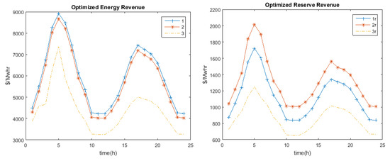
Figure 2.
Optimized revenue.
3.2. Analysis II: LMP as a Signal to Reserve Market
Locational marginal pricing is a way to calculate the outright purchase price of electric energy that reflects its value at different locations, by taking into account the network paradigm, load pattern, generation limits, and transmission constraints for the next MW required. The pricing of the next MW required to meet the CDR was defined as the locational contingency marginal reserve pricing or reserve LMP. The ACOPF gives a levy that includes the cost of energy, loss, and congestion. Figure 3 gives the maximum LMP in 24 h for the energy and reserve markets.
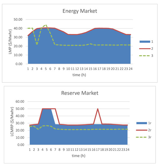
Figure 3.
Day-ahead maximum Locational Marginal Pricing (LMP) and Locational Contingency Marginal Reserve Pricing (LCMRP).
The maximum LMP for the energy market did not vary much for Market Models1 and 2. Market Model3 gave the minimum value of the maximum LMPs for the day. The maximum LMP for the reserve market was the minimum for Market Model 3r, compared to Market Models 1r and 2r.
The LMP varied in proportion with the demand quantity. The highest demand node, node 5, experienced the maximum price for the next MW required. Table 2 gives the nodes at which the price was the maximum for various energy and reserve market models. In the day-ahead energy market, the energy LMP was the maximum at node 5 throughout the day, with an average of maximum LMP (AML) of 37.41 $/MWhr for Market Model 1. The same node 5 also experienced the maximum LMP in Market Model 2, but with a reduced AML of 37.02 $/MWhr. In Market Model 3, the eventuality of the maximum LMP was shifted to other nodes 8, 11, 15, and 25, with a much-reduced value of maximum LMP and an average value of 25.21 $/MWhr.
Table 2.
LMP and LCMRP of various market models for the day-ahead market.
In the day-ahead reserve market, the LCMRP was maximum at node 5 in the case of Market Model 1r and was shifted to other nodes in Market Model 3r, with a much-reduced AML value of 22.40 $/MWhr. By means of simultaneous scheduling of wind farms and conventional thermal generators, the average value of the maximum LMP in the reserve market came close to the energy market. The next MW contingency reserve can be allocated at the price of nodal energy.
3.3. Analysis III: Impact of Wind Penetration on LMP
With the high penetration of wind farms, the negative LMP in various market models was converted to positive. The energy and contingency reserve markets were analyzed at nodes 5, 15, and 25. In the IEEE 30 bus system considered, the wind farms were installed at the above-mentioned nodes.
Figure 4 gives the energy prices for Market Models 1, 2, and 3, and the reserve prices for Market Models 1r, 2r, and 3r, in column 1 and column 2, respectively. The LMP at a node may be larger than the largest bid over all the available LSEs in the system. The energy market at node 5 gave a positive value of LMP for all the energy market models. The ECEs at these nodes paid the highest LMP for Market Model 1, a slightly reduced LMP for Market Model 2, and the lowest possible LMP for Market Model 3. The energy market at node 15 and 25 gave a negative value of LMP for Market Models 1 and 2 in the day-ahead market. A negative LMP at a node shows excess generation at that node. The negative LMPs at nodes 15 and 25 became positive in Market Model 3 in most hours. With the reduction in LMP at these nodes, the demand at various other nodes was supplied by these low-levy wind farms, which reduced the total operating cost.
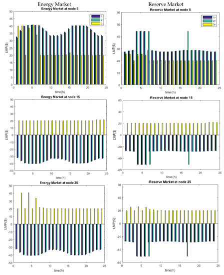
Figure 4.
The marginal prices for the energy and reserve markets.
Considering the reserve price/LCMRP for Market Models 1r, 2r, and 3r, the reserve market at node 5 and 11 gave a positive value of LMP for all reserve market modelsand a higher LMP at peak hourly loads. The IOPF implementation for contingency reserve analysis fetched an LMP at the reserve market lower than the lowest bid over all the available reserve-supplying LSEs. The reserve ECEs at these nodes paid a high value of LMP for Market Models 1r and 2r, excluding Market Model 3r. The reserve market at nodes 15 and 25 gave a negative value of LMP for all of Market Models 1r and 2r.In Market Model 3r, the negative LMP was converted to positive LMP, emphasizing the usage of available generation at that node. The contingency reserve bid which was submitted to the ISO was cleared at the cost of energy.
4. Conclusions
Better allocation in the energy market and reserve market can ensure benefits in terms of security and efficiency of operations. In this paper, an OPF with flexible thermal generators was extended by incorporating wind farms and then revamped to IOPF. The wind farms were scheduled more than the thermal generators when incorporated into the network, however, the thermal generators had the rock-bottom scheduling, because of the network constraints. Even though the lower cost generators (wind farms) were operated for maximum profit, there was a win-win situation for all the stakeholders. This paper compared the various market models of energy and reserve allocation in the deregulated power industry, considering the modified IEEE 30 bus system. The variation in generation schedule, the locational marginal pricing, and the negative LMP at various nodes were all analyzed. The hourly average LMP was calculated, as was the average value of maximum LMP in the day-ahead market, which helps ECEs to bid for the next day. All the computations were simulated using the MATLAB program. Future work will include the incorporation of solar and solar–thermal bundling as load-serving entities in large power system networks.
Author Contributions
Both authors contributed equally to this study. Both authors have read and agreed to the published version of the manuscript.
Funding
This research received no external funding.
Conflicts of Interest
The authors declare no conflict of interest.
Nomenclature
| Variables | |
| Bi | the reserve bid price of the LSE at bus i |
| Ei | the reserve bid price of the wind farm at bus i |
| the bid price of the LSE at bus i | |
| the bid price of the wind farm at bus i | |
| Pg | active power generation of thermal generators |
| Pw | active power generation of wind farms |
| Pd | the active power demand |
| DR | the down ramp of thermal generators |
| UR | the up ramp of thermal generators |
| V | the magnitude of the voltage at bus |
| δ | the phase angle of the voltage at bus |
| Subscript Index | |
| n | set of buses |
| ng | set of LSE/generator buses including swing bus |
| ns | set of slack bus |
| nd | set of buses with connected loads |
| nw | set of buses with connected wind farms |
| nl | set of transmission lines |
| g | the LSE/generator indicant |
| d | the ECE/demand indicant |
| gr | the LSE/generator reserve indicant |
| dr | the contingency demand indicant |
| w | the wind farm indicant |
| wr | the wind farm reserve indicant |
| k | the transmission line indicant |
| t | the time interval |
Appendix A
Table A1.
LSE cost coefficient profile of modified IEEE 30 bus system.
Table A1.
LSE cost coefficient profile of modified IEEE 30 bus system.
| LSE at Node | c | Up Ramp | Down Ramp | |||||
|---|---|---|---|---|---|---|---|---|
| 1 | 0.0384 | 20 | 0 | 0 | 360.2 | 65 | 85 | 135 |
| 2 | 0.25 | 20 | 0 | 0 | 140 | 30 | 30 | 65 |
| 5 | 0.01 | 40 | 0 | 0 | 100 | 30 | 30 | 35 |
| 8 | 0.01 | 40 | 0 | 0 | 100 | 30 | 30 | 25 |
| 11 | 0.01 | 40 | 0 | 0 | 100 | 30 | 30 | 20 |
| 13 | 0.01 | 40 | 0 | 0 | 100 | 30 | 30 | 30 |
Table A2.
Branch profile of the modified IEEE 30 bus system.
Table A2.
Branch profile of the modified IEEE 30 bus system.
| Branch | Resistance (p.u) | Reactance (p.u) | Half Line Charging Susceptance (p.u) |
|---|---|---|---|
| 1–2 | 0.0192 | 0.0575 | 0.0264 |
| 1–3 | 0.0452 | 0.1852 | 0.0204 |
| 2–4 | 0.0570 | 0.1737 | 0.0184 |
| 3–4 | 0.0132 | 0.0379 | 0.0042 |
| 2–5 | 0.0472 | 0.1983 | 0.0209 |
| 2–6 | 0.0581 | 0.1763 | 0.0187 |
| 4–6 | 0.0119 | 0.0414 | 0.0045 |
| 5–7 | 0.046 | 0.116 | 0.0102 |
| 6–7 | 0.0267 | 0.082 | 0.0085 |
| 6–8 | 0.012 | 0.042 | 0.0045 |
| 6–9 | 0 | 0.208 | 0 |
| 6–10 | 0 | 0.556 | 0 |
| 9–11 | 0 | 0.208 | 0 |
| 9–10 | 0 | 0.11 | 0 |
| 4–12 | 0 | 0.256 | 0 |
| 12–13 | 0 | 0.14 | 0 |
| 12–14 | 0.1231 | 0.2559 | 0 |
| 12–15 | 0.0662 | 0.1304 | 0 |
| 12–16 | 0.0945 | 0.1987 | 0 |
| 14–15 | 0.2210 | 0.1997 | 0 |
| 16–17 | 0.0824 | 0.1923 | 0 |
| 15–18 | 0.1073 | 0.2185 | 0 |
| 18–19 | 0.0639 | 0.1292 | 0 |
| 19–20 | 0.0340 | 0.0680 | 0 |
| 10–20 | 0.0936 | 0.209 | 0 |
| 10–17 | 0.0324 | 0.0845 | 0 |
| 10–21 | 0.0348 | 0.0749 | 0 |
| 10–22 | 0.0727 | 0.1499 | 0 |
| 21–22 | 0.0116 | 0.0236 | 0 |
| 15–23 | 0.1 | 0.2020 | 0 |
| 22–24 | 0.1150 | 0.01790 | 0 |
| 23–24 | 0.1320 | 0.2700 | 0 |
| 24–25 | 0.1885 | 0.3292 | 0 |
| 25–26 | 0.2544 | 0.3800 | 0 |
| 25–27 | 0.1093 | 0.2087 | 0 |
| 28–27 | 0 | 0.3960 | 0 |
| 27–29 | 0.2198 | 0.4153 | 0 |
| 27–30 | 0.3202 | 0.6027 | 0 |
| 29–30 | 0.2399 | 0.4533 | 0 |
| 8–28 | 0.0636 | 0.2000 | 0.214 |
| 6–28 | 0.0169 | 0.0599 | 0.065 |
Table A3.
Cost coefficient profile of windfarms.
Table A3.
Cost coefficient profile of windfarms.
| Wind Farms at Bus | Cut-in Speed m/s | |||
|---|---|---|---|---|
| 5 | 20 | 0 | Table A5 | 6 |
| 15 | 20 | 0 | 10 | |
| 25 | 20 | 0 | 5 |
Table A4.
Hourly demand for 24 h.
Table A4.
Hourly demand for 24 h.
| Hour | Demand Mw | Hour | Demand Mw |
|---|---|---|---|
| 1 | 166 | 13 | 170 |
| 2 | 196 | 14 | 185 |
| 3 | 229 | 15 | 208 |
| 4 | 267 | 16 | 232 |
| 5 | 283 | 17 | 246 |
| 6 | 272 | 18 | 241 |
| 7 | 246 | 19 | 236 |
| 8 | 213 | 20 | 225 |
| 9 | 192 | 21 | 204 |
| 10 | 161 | 22 | 182 |
| 11 | 160 | 23 | 161 |
| 12 | 160 | 24 | 160 |
Table A5.
Hourly wind speed for 24 h.
Table A5.
Hourly wind speed for 24 h.
| Hour | Wind Speed (m/s) | Hour | Wind Speed (m/s) | ||||
|---|---|---|---|---|---|---|---|
| W1 | W2 | W3 | W1 | W2 | W3 | ||
| 1 | 6 | 12 | 9 | 13 | 11 | 22 | 11 |
| 2 | 7 | 19 | 4 | 14 | 9 | 17 | 10 |
| 3 | 10 | 26 | 7 | 15 | 9 | 15 | 10 |
| 4 | 8 | 26 | 5 | 16 | 14 | 17 | 9 |
| 5 | 7 | 31 | 7 | 17 | 14 | 16 | 10 |
| 6 | 9 | 29 | 4 | 18 | 14 | 13 | 11 |
| 7 | 12 | 32 | 2 | 19 | 15 | 13 | 10 |
| 8 | 11 | 28 | 4 | 20 | 18 | 16 | 10 |
| 9 | 14 | 27 | 11 | 21 | 17 | 12 | 12 |
| 10 | 12 | 26 | 11 | 22 | 19 | 8 | 15 |
| 11 | 12 | 29 | 8 | 23 | 10 | 8 | 11 |
| 12 | 18 | 21 | 7 | 24 | 10 | 6 | 8 |
References
- Schweppe, F.C.; Caramanis, M.C.; Tabors, R.D.; Bohn, R.E. Spot Pricing of Electricity; Springer Science Business Media: Berlin/Heidelberg, Germany, 2013. [Google Scholar]
- Li, F.; Bo, R. Congestion and price prediction under load variation. IEEE Trans. Power Syst. 2009, 24, 911–922. [Google Scholar] [CrossRef]
- Bo, R.; Li, F. Probabilistic LMP forecasting considering load uncertainty. IEEE Trans. Power Syst. 2009, 24, 1279–1289. [Google Scholar]
- Cheng, X.; Overbye, T.J. An energy reference bus independent LMP decomposition algorithm. IEEE Trans. Power Syst. 2006, 21, 1041–1049. [Google Scholar] [CrossRef]
- Hu, Z.; Cheng, H.; Yan, Z.; Li, F. An iterative LMP calculation method considering loss distributions. IEEE Trans. Power Syst. 2010, 25, 1469–1477. [Google Scholar] [CrossRef]
- Baldick, R. Wind and energy markets: A case study of Texas. IEEE Syst. J. 2012, 6, 27–34. [Google Scholar] [CrossRef]
- Energy Explained—U.S. Energy Information Administration (EIA). Available online: www.eia.gov/energyexplained (accessed on 28 June 2019).
- Top 8 Best Dog Harnesses to Stop Pulling 2020 Reviews. Available online: www.uwig.org/windinmarketstableOct2011.pdf (accessed on 22 January 2016).
- Carta, J.A.; Ramirez, P.; Velazquez, S. A review of wind speed probability distributions used in wind energy analysis: Case studies in the Canary Islands. Renew. Sustain. Energy Rev. 2009, 13, 933–955. [Google Scholar]
- Hetzer, J.; David, C.Y.; Bhattarai, K. An economic dispatch model incorporating wind power. IEEE Trans. Energy Convers. 2008, 23, 603–611. [Google Scholar] [CrossRef]
- Cobos, N.G.; Arroyo, J.M.; Alguacil-Conde, N.; Street, A. Robust Energy and Reserve Scheduling under Wind Uncertainty Considering Fast-Acting Generators. IEEE Trans. Sustain. Energy 2018. [Google Scholar] [CrossRef]
- Wind Farms Construction. Available online: www.windfarmbop.com/is-wind-energy-really-unpredictable (accessed on 28 June 2019).
- Reddy, S.S. Optimal scheduling of thermal-wind-solar power system with storage. Renew. Energy 2017, 101, 1357–1368. [Google Scholar]
- Song, Z.; Goel, L.; Wang, P. Optimal spinning reserve allocation in deregulated power systems. IEEE Proc. -Gener. Transm. Distrib. 2005, 152, 483–488. [Google Scholar] [CrossRef]
- Yu, Y.; Luh, P.B.; Litvinov, E.; Zheng, T.; Zhao, J.; Zhao, F.; Schiro, D.A. Transmission contingency-constrained unit commitment with high penetration of renewables via interval optimization. IEEE Trans. Power Syst. 2016, 32, 1410–1421. [Google Scholar] [CrossRef]
- Sundaram, A.; Abdullah Khan, M. Market Clearing and Settlement Using Participant Based Distributed Slack Optimal Power Flow Model for a Double-Sided Electricity Auction Market—Part II. Electr. Power Compon. Syst. 2018, 46, 533–543. [Google Scholar] [CrossRef]
- Rodriguez, C.P.; Anders, G.J. Bidding strategy design for different types of electric power market participants. IEEE Trans. Power Syst. 2004, 19, 964–971. [Google Scholar] [CrossRef]
- Prabavathi, M.; Gnanadass, R. Energy bidding strategies for the restructured electricity market. Int. J. Electr. Power Energy Syst. 2015, 64, 956–966. [Google Scholar] [CrossRef]
- Wang, Q.; Chang, L. An intelligent maximum power extraction algorithm for inverter-based variable speed wind turbine systems. IEEE Trans. Power Electron. 2004, 19, 1242–1249. [Google Scholar] [CrossRef]
- Wood, A.J.; Wollenberg, B.F.; Sheble, G.B. “Unit Commitment” in Power Generation, Operation and Control, 3rd ed.; Wiley: Hoboken, NJ, USA, 2014; pp. 147–148. [Google Scholar]


© 2020 by the authors. Licensee MDPI, Basel, Switzerland. This article is an open access article distributed under the terms and conditions of the Creative Commons Attribution (CC BY) license (http://creativecommons.org/licenses/by/4.0/).