Article

Preventive Security-Constrained Optimal Power Flow with Probabilistic Guarantees

State Key Laboratory of Advanced Electromagnetic Engineering and Technology, Huazhong University of Science and Technology, 1037 Luoyu Road, Wuhan 430074, China
*
Author to whom correspondence should be addressed.
Energies 2020, 13(9), 2344; https://doi.org/10.3390/en13092344
Submission received: 17 March 2020 / Revised: 27 April 2020 / Accepted: 30 April 2020 / Published: 8 May 2020
(This article belongs to the Special Issue Power System Simulation, Control and Optimization)

Abstract

:
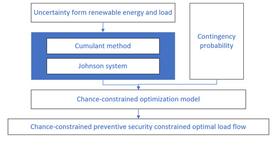
The traditional security-constrained optimal power flow (SCOPF) model under the classical N-1 criterion is implemented in the power industry to ensure the secure operation of a power system. However, with increasing uncertainties from renewable energy sources (RES) and loads, the existing SCOPF model has difficulty meeting the practical requirements of the industry. This paper proposed a novel chance-constrained preventive SCOPF model that considers the uncertainty of power injections, including RES and load, and contingency probability. The chance constraint is used to constrain the overall line flow within the limits with high probabilistic guarantees and to significantly reduce the constraint scales. The cumulant and Johnson systems were combined to accurately approximate the cumulative distribution functions, which is important in solving chance-constrained optimization problems. The simulation results show that the model proposed in this paper can achieve better performance than traditional SCOPF.

Graphical Abstract

1. Introduction

The growth in renewable energy sources (RES) and charging loads in recent years, such as wind power, photovoltaics and electric vehicle, has brought considerable economic benefits; however, the uncertainty of power injections has increased, which leads to increased operational risks [1,2,3], especially for highly-loaded power systems. The increasing uncertainty of operation increases the need for new criteria, dispatch tools and control methods to better balance operational security and costs [4].
Optimal power flow (OPF) is the fundamental dispatch and planning tool that is used to minimize operational costs while ensuring the security of the normal state, and security-constrained optimal power flow (SCOPF) [4,5,6,7] is an extended form of OPF that considers the classical N-1 criterion. Unlike OPF, which only considers a single system topology (normal state), SCOPF typically ensures that the system state remains within the operational limits when unexpected component outages (contingency set) occur. However, with the emergence of uncertainties in the power system, several drawbacks of traditional SCOPF have become apparent and these need to be addressed. These include:
1. Traditional SCOPF does not consider the influence of the uncertainty of RES and loads, and it cannot provide a robust solution because increasing uncertainty makes the operational state more stochastic and may lead to frequent violations of the N-1 criterion.
2. Traditional SCOPF disregards the probability of a contingency occurring; in other words, it considers the occurrence probability to be 1 for every contingency in a contingency set [4]. Obviously, this does not match the actual situation because the probability of a contingency is usually very low.
3. The scale of the SCOPF problem is highly related to the scale of the power system and the number of contingencies. This means that for a large power system where a large number of contingencies are considered, the calculation burden is high, and directly solving a SCOPF problem in a short time is quite challenging.

1.1. Literature Review

Numerous studies have attempted to address the drawbacks of the traditional SCOPF model.
To the best of the authors’ knowledge, there are currently two strategies to reduce the calculation burden of traditional SCOPF and make it easier to solve. One strategy uses a contingency filtering (CF) [8,9] technique to reduce the number of contingencies. Usually, an index that ranks the severity of a contingency is used to filter contingencies; thus, only the contingency that exceeds the severity threshold is included in the contingency set. However, choosing the severity threshold itself is a challenge, for example, a very severe contingency may have a very low probability of occurring, and controlling it through SCOPF may result in excessive costs. The second strategy is to use Benders decomposition (BD) [10,11,12] to decompose the original SCOPF problem into a master problem and several subproblems. In this way, parallel computing technology can be used to improve the computing efficiency; however, BD requires convexity of the feasible region, which is not guaranteed in an SCOPF problem [12].
The concept of risk-based SCOPF [13,14,15] has been proposed as a method that comprehensively considers the probability and severity of contingencies. The risk of a contingency is defined as the product of the probability and severity of a contingency. Risk-based SCOPF uses risk as constraints to achieve a tradeoff between economic and security. This method relaxes the constraints of a single contingency [14] but controls the total risk of a contingency set to a certain level. Although the security and economy of power system operations are enhanced by risk-based SCOPF, the uncertainty of RES and load are not taken into consideration because measuring system risk under uncertainty is a challenging task. Moreover, the optimization formulation of risk-based SCOPF is complicated, and the calculation time is 4–7 times that of traditional SCOPF [14], which makes it difficult to apply in a real-time dispatch.
Chance-constrained optimization (CCO) [16,17,18,19,20,21,22,23,24,25,26] is a promising method to handle the uncertainty in power systems and it has been successfully applied to many problems. Instead of rigid constraint, CCO ensures a certain level of probability that the constraint is satisfied. The work of Bienstock [19] provides a solid foundation for incorporating CCO with OPF. This model was further extended in [22] to incorporate corrective SCOPF. Li et al. [23] provided a novel transmission expansion planning approach based on CCO and BD. Liu et al. [24], proposed solutions based on CCO for peak power shaving and frequency regulation in microgrids. Based on CCO, a day-ahead scheduling approach is proposed in [25] and a volt/var control approach is provided in [26]. Although CCO has been successfully applied to a variety of problems, the probability distribution of the uncertainty source is usually assumed to follow a Gaussian distribution. Studies [27,28,29] have indicated that the distribution of wind power forecast error and photovoltaic power is very different from a Gaussian distribution; therefore, the existing models should be improved so that they are able to handle arbitrary distributions. Moreover, there are few CCO models that consider contingency probability.

1.2. Contributions

This paper proposes a novel chance-constrained preventive SCOPF model (CC-PSCOPF) that is an improvement on the traditional preventive SCOPF (PSCOPF) model. The main contributions are as follows:
1. A novel CC-PSCOPF model is proposed to improve the overall operational reliability. The model considers contingency probability and the uncertainty of power injections (including RES and load).
2. Instead of using the large-scale line flow limits of traditional PSCOPF, the probability distribution of the overall line flow is obtained and constrained in the proposed optimization model, which significantly reduces the constraint scale.
3. The cumulant and Johnson systems are combined in this paper to accurately approximate the cumulative distribution function (CDF) of an arbitrary distribution random variable, which only requires the first four orders of moment information.
The remainder of this paper is organized as follows: Section 2 reviews the traditional PSCOPF model. Section 3 describes the formulation of the proposed CC-PSCOPF, and a cumulative distribution function (CDF) approximation method based on cumulants and the Johnson system is also introduced. A case study is presented in Section 4 to test the performance of the proposed model. Section 5 presents our discussion and conclusions.

2. Review of Traditional PSCOPF

There are two types of SCOPF: PSCOPF and corrective SCOPF (CSCOPF). Using PSCOPF, pre-contingency controls are the only measures allowed to ensure that the system always operates in a state where any single component outage does not lead to constraint violations. This indicates that the operational state determined by PSCOPF simultaneously satisfies the pre- and post-contingency constraints. Different from PSCOPF, CSCOPF determines an operational state that allows post-contingency constraint violations, and it ensures that there are adequate post-contingency control measures, e.g., generator re-dispatch, topology reconfiguration and load shedding to eliminate post-contingency constraint violations. PSCOPF is safer, while CSCOPF is more economical [4].
This paper focuses on improving the traditional PSCOPF, and the proposed optimization model attempts to improve the overall security performance of the system operation through pre-contingency controls.
The DC-based PSCOPF model is reviewed in this section, as it provides the foundation for the optimization model proposed in this paper. DC approximation is used in this paper because it provides a convex guarantee that the optimization problem is tractable [20].
The objective function of DC-based PSCOPF minimizes the system’s operational cost in the normal state, and it is expressed as follows:
min   G i = 1 N G P G i T c 2 i P G i + c 1 i T P G i + c 0 i
where N G is the number of generators; P G i is the ith generator output in the normal state, which is the control variable of the optimization model; and c 2 i ,   c 1 i ,   and   c 0 i are the quadratic, linear and constant cost coefficients, respectively.
The equality and inequality constraints of the PSCOPF model are as follows:
G i = 1 N G P G i + R i = 1 N R P R i = D i = 1 N D P D i
P ¯ G i P G i P ¯ G i                 i
G i = 1 N G A G i k P G i + R i = 1 N R A R i k P R i D i = 1 N D A D i k P D i P ¯ l         i , k , l
P ¯ l G i = 1 N G A G i k P G i + R i = 1 N R A R i k P R i D i = 1 N D A D i k P D i         i , k , l
These include the power balance of the system (2), the generator output limits (3) and the line flow limits (4) and (5). N R and N D are the number of RES and loads, respectively, in the system; P R i and P D i are the forecast power injections of the ith RES and load; P ¯ G i and P ¯ G i are the ith generator’s minimal output and maximum output, respectively; P ¯ l and P ¯ l are the lower and upper limits of the ith line flows; superscript k is the index of system topology; k = 0 indicates the normal state system topology, while k 1 indicates the contingency system topology; and A G i k ,   A R i k and A D i k are the power transmission distribution factors (PTDFs) of the ith generator, RES and load under system topology k, respectively. The PTDF can be obtained from the line susceptance matrix and bus susceptance matrix, and details can be found in [6].
The traditional DC-based PSCOPF optimization model is a typical quadratic programming problem that can be solved by common commercial solvers. As discussed in the introduction, the uncertainties of power injections and contingency probability are not considered in this model; therefore, the operational state obtained by this model is not robust to uncertainty and may be very costly. The constraint number of this model is 1 + N G + 2 × N l × N k , where N l is the number of lines and N k is the scale of the contingency set. Obviously, when the system scale is large with a large contingency set, the constraint number of this model is quite high, which significantly increases the calculation burden.

3. Formulation of the Proposed Optimization Model

3.1. Modeling of Uncertainties

The forecast error of the RES and load is the main source of uncertainty, which is the deviation of the forecast value from the actual value. The forecast error can be seen as a continuous random variable and described by a continuous probability distribution model. Therefore, the actual power injection of RES and loads can be modeled as a forecast value plus a continuous random variable that represents forecast error:
{ P ˜ R i = P R i + δ R i P ˜ D i = P D i + δ D i         i
where P ˜ R i and P ˜ D i are the actual power injection of the ith RES and load, respectively, and δ R i and δ D i are random variables that represent the forecast error of the power injection of the ith RES and load, respectively.
The proper distribution model to describe forecast error depends on the type of power injection, forecasting scale [27], etc. For instance, the forecast error of a load is usually assumed to follow a Gaussian distribution, while the beta distribution [28] is an appropriate choice to describe the short-term forecast error of wind power. Although there are many distribution models that can be used to describe a forecast error, the optimization model proposed in this paper is not sensitive to the distribution used. The first four order moments of a distribution model is the only information that is required and this can be obtained from historical data This moment information is used to approximate the CDF of a random variable, which is discussed in the following section.
The line flow under a single system topology is linearly dependent on power injections; when considering uncertainty, its expression is:
P l k = G i = 1 N G A G i k P G i + R i = 1 N R A R i k P ˜ R i D i = 1 N D A D i k P ˜ D i = ( G i = 1 N G A G i k P G i + R i = 1 N R A R i k P R i D i = 1 N D A D i k P D i ) + ( R i = 1 N R A R i k δ R i D i = 1 N D A D i k δ D i )         l , k
where P l k is the lth line flow under the kth system topology. The term in the first bracket of Equation (7) is the line flow part formed by forecast power injections, which is consistent with the traditional PSCOPF. The term in the second bracket of Equation (7) is the uncertainty part of a line flow, which is the linear combination of the forecast error of power injections of RES and load.
The overall line flow probability distribution, which comprehensively considers the influence of the uncertainty of power injection and system topology is our concern. Therefore, the occurrence probability of a system topology, or the so-called contingency probability, should be obtained.
The Poisson distribution [30] is used in this paper to describe the occurrence probability of a system topology:
P r ( s k ) = 1 e λ t
where s k is the kth contingency’s system topology, P r ( s k ) is the corresponding occurrence probability, e is the base of the natural logarithm and λ t is the failure rate of the component. Note that the failure rate can be modified according to the external weather conditions. An approach to calculate the failure rate under different weather conditions (normal, adverse and major adverse) is provided in [31].
For each contingency, an occurrence probability can be obtained from Equation (8). We assume that contingencies outside the contingency set will have little impact on system operation, so the probability of the normal state is approximated and expressed as:
P r ( s 0 ) = 1 k = 1 N k P r ( s k )
Considering the uncertainty of power injections and the probability of contingency, the overall line flow P l can be obtained through the law of total probability theory, and it is expressed as:
P l = P r ( s 0 ) P l 0 + P r ( s 1 ) P l 1 + P r ( s N k ) P l N k         l = k = 0 N k G i = 1 N G A G i k P G i P r ( s k ) + k = 0 N k R i = 1 N R A R i k P R i P r ( s k ) k = 0 N k R i = 1 N R A D i k P D i P r ( s k ) + k = 0 N k R i = 1 N R A R i k δ R i P r ( s k ) k = 0 N k R i = 1 N R A D i k δ D i P r ( s k )                 l
Obviously, the probability distribution of the overall line flow P l can be regarded as the weighted average of the line flow probability distribution under each system topology.

3.2. Chance-Constrained Optimization

In this section, we briefly introduce the CCO, which also underpins the model proposed in this paper.
CCO is an important tool proposed by Charnes and Cooper [16,17] for solving optimization problems under uncertainties. The general form of a CCO problem is expressed as follows:
min f ( x , ξ ) s . t . g ( x , ξ ) = 0   Pr { h ( x , ξ ) 0 } 1 α
where f ( · ) is the objective function, g ( · ) is the equality constraint, h ( · ) is the inequality constraint, x is the decision variable, ξ is the uncertainty variable and α is the reliability parameter representing the allowed constraint violation level.
Under the CCO, the inequality constraint is formed as the chance constraint and ensures that the constraint h ( · ) is satisfied with probability 1 α at least. The original CCO problem is often transformed into an equivalent deterministic form to facilitate the solution [20,24].

3.3. Chance-Constrained PSCOPF Model

In this section, we present a novel CC-PSCOPF model that considers the uncertainties of power injections and the probability of contingency.
The goal function, power balance constraint and generator output limit of the proposed CC-PSCOPF are the same as those of the traditional PSCOPF model, as Equations (1)–(3) show. The key improvement is the modeling of the line flow inequality constraints.
Instead of line flow constraints under each system topology used in traditional PSCOPF, the overall line flow P l is constrained in CC-PSCOPF. As analyzed in the previous section, P l is a random variable; therefore, the chance constraint is used to place it in a certain range with a high probability, and it is expressed as follows:
P r { P l P ¯ l }   α l +         l
P r { P l P ¯ l }   α l         l
where α l + and α l are predefined violation levels. Considering the low occurrence probability of contingencies, α l + and α l should be carefully defined.
A comparison of Equations (12) and (13) to Equations (4) and (5) shows that the optimization model proposed in this paper has the following significant advantages:
1. The uncertainty of power injections and contingency occurrence probability are considered through P l . Even with the influence of various uncertainties, the operational state obtained by CC-PSCOPF has a high probability of ensuring that constraints are not violated. Obviously, the operational state is more robust to uncertainties compared to traditional PSCOPF.
2. The violation level for different lines is adjustable; for critical lines, the violation level could be adjusted lower to ensure operational safety, while for noncritical lines, the violation level could be increased to save control costs.
3. The scale of the line flow constraint is significantly reduced, which is only related to the number of lines in the system, allowing the optimization problems to be solved more efficiently.
4. As the occurrence probabilities of the contingency and chance constraints are used in this model, some contingencies that have quite low probability but high control costs are ignored in the optimization model, which helps to reduce the control costs. The control measures of these low probability contingencies can be solved using a separate accident plan.
However, solving an optimization problem with chance constraints directly is a challenging task. In this paper, chance constraints are transformed into deterministic linear constraints based on the cumulant and Johnson systems in the following section, which ensures that the CC-PSCOPF is tractable and solved efficiently.

3.4. Deterministic Reformulation of CC-PSCOPF

The main challenge of solving the proposed model is how to handle the two chance constraints related to overall line flows. In this section, these two constraints are converted into deterministic linear constraints. Through conversion, the optimization model becomes a linear constrained convex optimization problem that is easy to solve.
For convenience, the factors that determine the overall line flow P l are divided into two terms:
P l , c o n t r o l = k = 0 N k G i = 1 N G A G i k P G i P r ( s k ) P l , u n c e r t a i n t y = k = 0 N k R i = 1 N R A R i k P R i P r ( s k ) k = 0 N k R i = 1 N R A D i k P D i P r ( s k ) + k = 0 N k R i = 1 N R A R i k δ R i P r ( s k ) k = 0 N k R i = 1 N R A D i k δ D i P r ( s k )         l
where P l , c o n t r o l k is the line flow part determined by the control variable, which varies with the output of the generators, and P l , u n c e r t a i n t y is the line flow part determined by power injections of the RES and load, which is a random variable.
Substituting Equation (14) into Equation (12) yields:
P r { P l , u n c e r t a i n t y P ¯ l P l , c o n t r o l }   1 α l +         l
Note that P l , u n c e r t a i n t y is the uncertainty part of the overall line flows, and we can obtain:
C D F l , u n c e r t a i n t y ( P ¯ l P l , c o n t r o l )   1 α l + P ¯ l P l , c o n t r o l C D F l , u n c e r t a i n t y 1 ( 1 α l + )         l
where C D F l , u n c e r t a i n t y and C D F l , u n c e r t a i n t y 1 are the CDF and inverse CDF of P l , u n c e r t a i n t y , respectively. Similar to Equation (16), by substituting Equation (14) into (13), we can obtain:
P ¯ l P l , c o n t r o l C D F l , s t o c h a s t i c 1 ( α l )         l
To replace Equations (12) and (13) with deterministic linear constraints Equations (16) and (17), C D F l , u n c e r t a i n t y 1 should be obtained. Traditionally, C D F l , u n c e r t a i n t y is obtained from Monte Carlo simulation (MCS), which performs a numerical search for the C D F l , u n c e r t a i n t y 1 [20]; however, this is time consuming. Moreover, MCS is difficult to implement in the absence of samples. Here, this procedure is improved by using the cumulant and Johnson system to obtain C D F l , u n c e r t a i n t y 1 .

3.4.1. The Cumulant

The cumulant [32,33] is an alternative moment of a continuous probability distribution, and the relationship between the cumulant κ and moment m is as follows:
κ 1 = m 1 κ 2 = m 2 m 1 2 κ 3 = m 3 3 m 1 m 2 + 2 m 1 3 κ 4 = m 4 2 m 2 2 4 m 1 m 3 + 12 m 1 2 m 2 6 m 1 4
Cumulants have two important characteristics. One is homogeneity. For a random variable x, the nth cumulant is homogeneous of order r:
κ r ( a x ) = a r κ r ( x )
The other is additivity; for two independent random variables x and y , and z = x + y , then:
κ r ( z ) = κ r ( x ) + κ r ( y )
The uncertainty part of line flow under a single system topology is the linear combination of δ R i and δ D i . As we know the first four order moments of δ R i and δ D i in advance, using Equation (18) and the characteristics of the cumulant, the first four order moments of the uncertainty part of the line flow under a single system topology can be obtained.

3.4.2. The Johnson System

Previous works [34,35] have shown that the Johnson system is a reliable and accurate method for obtaining CDF compared to the commonly used Gram-Charlier series [32] or Cornish-Fisher series [33]; therefore, it is used here to obtain the CDF of the uncertainty part of the line flow under a single system topology.
The Johnson system is a 4-parameter transformation system that uses the following function to transform the standard Gaussian variable u into a variable x that follows an unknown arbitrary probability distribution:
x = c + d × f 1 ( u a b )
where a and b are the shape parameters, c is the position parameter, and d is the scale parameter. The function f 1 ( · ) takes 4 forms to distinguish different distribution families:
{ S L : f 1 ( u a b ) = e ( u a ) / b S U : f 1 ( u a b ) = ( e ( u a ) / b e ( u a ) / b ) / 2 S B : f 1 ( u a b ) = 1 / ( 1 + e ( u a ) / b ) S N : f 1 ( u a b ) = u a b
where SL is the family of lognormal distributions, SU is the family of unbounded distributions, which means the range of variables is unlimited, SB is the family of bounded distributions, and SN is the family of Gaussian distributions.
If the first four order moments of random variable x (the uncertainty part of the line flow in this paper) are available, the moment-based algorithm [36] can be used to obtain the parameters of the Johnson system, and the CDF of x is a function of the CDF of the standard Gaussian variable, which can be obtained easily.
The CDF of the uncertainty part of the line flow under each system topology is obtained. Based on the law of total probability, C D F l , u n c e r t a i n t y is calculated through the weighted average of each CDF of the uncertainty part of the line flow, and its inverse function C D F l , u n c e r t a i n t y 1 can be efficiently calculated.

4. Case Study

In this section, we discuss the performances of traditional PSCOPF and CC-PSCOPF, which were tested on two test systems. The optimization problem was solved by Ipopt [37] on a PC with a 2.8-GHz CPU and 16 GB RAM.

4.1. Description of the Test System

A modified IEEE-30 test system [38] was used here to analyze the characteristics of these two optimization formulations and a modified IEEE-108 test system [38] was used to evaluate the efficiency of these two methods. The IEEE-30 test system was modified to add two wind power generators at bus 7 and 12, which are representative of a RES power injection. Similarly, the IEEE-108 test system was modified to add four power generators at bus 44, 50, 88 and 98. The rated power of the wind power generators is 80 MW, the forecast outputs of wind power generators are assumed to be 0.8 p.u., and forecast error is assumed to follow a beta distribution: Beta (0.83, 1.82). The forecast error of the load at each bus is assumed to follow a Gaussian distribution, with the means of the power injections equal to those of the base case data and standard deviations equal to 5% of the means.
All N-1 contingencies are included in the contingency set, the occurrence probability of each contingency is assumed to be 0.01, and the violation level α l + is set at 1% for all lines.

4.2. CDF Approximation Performance of the Proposed Method

Obtaining an accurate CDF curve, especially in the tail area, is the basis for accurately solving the chance-constrained optimization. This section presents the results to show that the proposed cumulant + Johnson system can accurately and efficiently approximate a CDF curve.
The proposed method is compared with 10,000 MCS, the commonly used cumulant + Gram-Charlier series proposed in [25], and a CDF curve based on the assumption that wind power forecast error follows a Gaussian distribution.
The CDF curve of line 4-6 flow and line 16-17 flow under the normal state is chosen here as representative and to visually show the approximation ability of the evaluated method. The CDF curves are shown in Figure 1a,b.
The average root mean square (ARMS) [18] is also introduced here to quantitatively indicate the accuracy of the CDF approximation. The smaller the ARMS value is, the more accurately the method approximates the CDF curve. Table 1 shows the ARMS values of the evaluated methods.
The results in Figure 1 and Table 1 show that the cumulant + Johnson system approximates the CDF curve best and only a small amount of error exists, while the curve approximated by cumulant + Johnson and Gaussian assumptions shows significant deviation, especially in the tail area.
Moreover, the method proposed in this paper has an advantage over MCS; that is, MCS cannot be implemented when only the moment information of power injections is available, while the method proposed in this paper can provide a reliable CDF curve.

4.3. Solutions of Different Optimization Formulations

The generation costs for the two optimization approaches are listed in Table 2. The cost of CC-PSCOPF is higher because it considers the uncertainty of power injections and gives a high probabilistic guarantee that line flows limit violations will not happen.
Because the chance constraint is a soft constraint and the Gaussian distribution is an unbounded distribution, there are always extreme values that cause line flow violations. Based on the generator output schemes given by these two problem formulations, we implemented MCS with 10,000 samples to observe the actually probability of line flow violations.
The average violation probability and the maximum violation probability were introduced to illustrate the effectiveness of the proposed method. These two indices are listed in Table 3. It is obvious that the chance constraint works; the maximum violation probability under CC-PSCOPF equals 0.01, which is equal to the preset violation level, while under PSCOPF, the same index significantly exceeds the violation level. Both the average and maximum violation probability are smaller under CC-PSCOPF, which indicates that the proposed method provides a more robust operational state than PSCOPF.
Moreover, although the goal of the proposed method is to improve the operational reliability by controlling the violation probability of line flows in the overall situation rather than the violation probability under a specific contingency system topology, it is interesting to note that CC-PSCOPF effectively reduces violations under a single contingency system topology. We counted the number of contingencies N V where the line flow violation probability exceeds the violation level. For contingencies with violations, the average number of line flows N a l v and maximum number of line flows N m l v that exceeds the violation level were also counted. The statistical data are listed in Table 3. Obviously, CC-PSCOPF effectively reduces N V , N a l v and N m l v , and this indicates that more contingencies are effectively controlled.
The line flow of 15–18 was chosen as representative to visually show the flow probability distributions under these two formulations. The histograms of line flow are shown in Figure 2a,b, respectively. It is clear that more PSCOPF samples fall outside of the line limits.

4.4. Influence of the Value of Violation Level

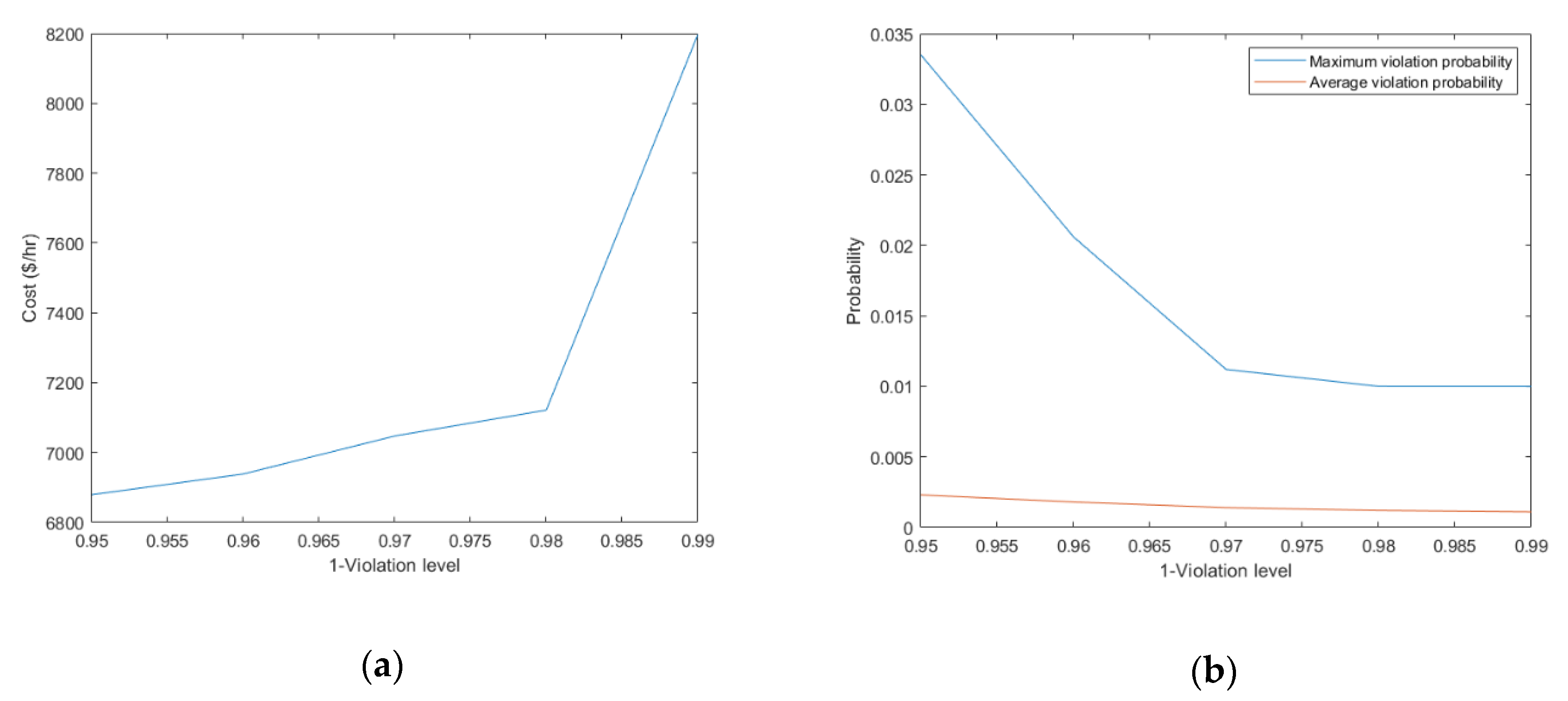
Changing the violation level influences the solution of CC-PSCOPF. Figure 3 shows the change in the generation cost and violation probability of CC-PSCOPF with different violation levels.
As Figure 3 shows, with increasing violation level, the generation cost of CC-PSCOPF decreases, and inevitably, this causes a larger probability of constraint violations.
Obviously, the contradiction between power generation costs and operational security can be balanced by adjusting the violation level. As different transmission system operators have different requirements for line constraint violation probability, how to determine the optimal violation will be explored in subsequent studies. Note that, theoretically, the violation level can be set at 0 to completely eliminate the constraint violations, but this is not worth the gains. On the one hand, this will cause a surge in control costs, and on the other hand, it is easy to make the problem infeasible, especially when the uncertainty of power injection is large. Moreover, the violation level of different lines can be set to different values. For the critical lines, appropriately reducing the violation level can improve safety, and for non-critical lines, increasing the violation level appropriately can reduce generation costs. Obviously, CC-PSCOPF is more flexible compared with traditional PSCOPF, which can only balance the control costs and security by adjusting the contingency set.

4.5. Efficiency of the Proposed Method

The time consumption of PSCOPF and CC-PSCOPF was tested on the IEEE-30 test system and a larger-scale system, the IEEE-118 test system. The constraint numbers and time consumption of these two optimization formulations are listed in Table 4. It is evident that the constraint numbers significantly influence the efficiency of the optimization model. CC-PSCOPF is much faster than PSCOPF because the line limit constraints of all the system topologies are reduced to the same number of lines by the law of total probability.

5. Conclusions

Currently, and in the future, increasing uncertainty brings challenges for power systems. The traditional SCOPF under strict N-1 criterion can barely meet the requirements of a secure operation. To obtain an operational state that is robust to uncertainties and to improve the overall operational reliability, a novel CC-PSCOPF was proposed in this paper. The probability distribution of the overall line flow is obtained and constrained within the limits with a high probability guarantee in the proposed optimization model. This type of constraint greatly reduces the number of constraints for the entire optimization problem, and additionally, the violation probability of each line can be flexibly adjusted as needed. In addition, the cumulant and Johnson systems are proposed to approximate the CDF curves, so the chance-constraint optimization model proposed in this paper is not limited to the Gaussian distribution assumption.
The proposed CC-PSCOPF can be used to improve the safety level of a system’s operation, especially for a system with a high level of RES penetration. How to determine the optimal violation level and correlations between uncertainty sources will be investigated in subsequent studies.

Author Contributions

H.L. conceived and designed the study; this work was performed under the guidance of Z.Z., B.Z. and X.Y. All authors have read and agreed to the published version of the manuscript.

Funding

This research received no external funding.

Acknowledgments

The authors gratefully acknowledge the support of the National High Technology Research and Development Program of China (863 Program): No. 2015AA050201.

Conflicts of Interest

The authors declare no conflict of interest.

References

  1. Li, X.; Zhang, X.; Wu, L.; Lu, P.; Zhang, S. Transmission Line Overload Risk Assessment for Power Systems with Wind and Load-Power Generation Correlation. IEEE Trans. Smart Grid. 2015, 6, 1233–1242. [Google Scholar] [CrossRef]
  2. Duan, Y.; Zhang, B. Security risk assessment using fast probabilistic power flow considering static power-frequency characteristics of power systems. Int. J. Electr. Power Energy Syst. 2014, 6, 53–58. [Google Scholar] [CrossRef]
  3. Da Silva, A.M.L.; De Castro, A.M. Risk Assessment in Probabilistic Load Flow via Monte Carlo Simulation and Cross-Entropy Method. IEEE Trans. Power Syst. 2019, 34, 1193–1202. [Google Scholar] [CrossRef]
  4. Capitanescu, F. Critical review of recent advances and further developments needed in AC optimal power flow. Electr. Power Syst. Res. 2016, 136, 57–68. [Google Scholar] [CrossRef]
  5. Monticelli, A.; Pereira, M.V.F.; Granville, S. Security-constrained optimal power flow with post-contingency corrective rescheduling. IEEE Trans. Power Syst. 1987, 2, 175–182. [Google Scholar] [CrossRef]
  6. Hinojosa, V.H.; Gonzalez-Longatt, F. Preventive Security-Constrained DCOPF Formulation Using Power Transmission Distribution Factors and Line Outage Distribution Factors. Energies 2018, 11, 1497. [Google Scholar] [CrossRef] [Green Version]
  7. Xu, Y.; Dong, Z.Y.; Zhang, R.; Wong, K.P.; Lai, M.Y. Solving Preventive-Corrective SCOPF by a Hybrid Computational Strategy. IEEE Trans. Power Syst. 2014, 29, 1345–1355. [Google Scholar] [CrossRef]
  8. Alsac, O.; Bright, J.; Prais, M.; Stott, B. Further developments in LP-based optimal power flow. IEEE Trans. Power Syst. 1990, 5, 697–711. [Google Scholar] [CrossRef]
  9. Capitanescu, F.; Glavic, M.; Ernst, D.; Wehenkel, L. Contingency filtering techniques for preventive security-constrained optimal power flow. IEEE Trans. Power Syst. 2007, 22, 1690–1697. [Google Scholar] [CrossRef]
  10. Li, Y.; McCalley, J.D. Decomposed SCOPF for improving efficiency. IEEE Trans. Power Syst. 2009, 24, 494–495. [Google Scholar]
  11. Fu, Y.; Shahidehpour, M.A.C. Contingency dispatch based on security-constrained unit commitment. IEEE Trans. Power Syst. 2006, 21, 897–908. [Google Scholar] [CrossRef]
  12. Granville, S.; Lima, M.C.A. Application of decomposition techniques to VAr planning: Methodological and computational aspects. IEEE Trans. Power Syst. 1994, 9, 1780–1787. [Google Scholar] [CrossRef]
  13. Wang, Q.; McCally, J.D. Risk and “N-1” Criteria Coordination for Real-Time Operations. IEEE Trans. Power Syst. 2013, 28, 3505–3506. [Google Scholar] [CrossRef]
  14. Wang, Q.; McCally, J.D.; Zheng, T.X.; Litvinov, E. Solving corrective risk-based security-constrained optimal power flow with Lagrangian relaxation and Benders decomposition. Int. J. Electr. Power Energy Syst. 2016, 75, 255–264. [Google Scholar] [CrossRef]
  15. Roald, L.; Vrakopoulou, M.; Oldewurtel, F.; Andersson, G. Risk-based optimal power flow with probabilistic guarantees. Int. J. Electr. Power Energy Syst. 2015, 72, 66–74. [Google Scholar] [CrossRef] [Green Version]
  16. Charnes, A.; Cooper, W.; Symonds, G. Cost horizons and certainty equivalents: An approach to stochastic programming of heating oil. Manag. Sci. 1958, 4, 235–263. [Google Scholar] [CrossRef]
  17. Charnes, A.; Cooper, W. Deterministic equivalents for optimizing and satisficing under chance constraints. Oper. Res. 1963, 11, 18–39. [Google Scholar] [CrossRef]
  18. Zhang, Z.S.; Sun, Y.Z.; Gao, D.W.; Lin, J.; Cheng, L. A Versatile Probability Distribution Model for Wind Power Forecast Errors and Its Application in Economic Dispatch. IEEE Trans. Power Syst. 2013, 28, 3114–3125. [Google Scholar] [CrossRef]
  19. Bienstock, D.; Chertkov, M.; Harnett, S. Chance-Constrained Optimal Power Flow: Risk-Aware Network Control under Uncertainty. SIAM Rev. 2014, 56, 461–495. [Google Scholar] [CrossRef]
  20. Wang, Z.W.; Shen, C.; Liu, F.; Wu, X.Y.; Liu, C.C.; Gao, F. Chance-Constrained Economic Dispatch With Non-Gaussian Correlated Wind Power Uncertainty. IEEE Trans. Power Syst. 2017, 32, 4880–4893. [Google Scholar] [CrossRef]
  21. Venzke, A.; Halilbasic, L.; Markovic, U.; Hub, G.; Chatzivasileiadis, S. Convex Relaxations of Chance Constrained AC Optimal Power Flow. IEEE Trans. Power Syst. 2018, 33, 2829–2841. [Google Scholar] [CrossRef] [Green Version]
  22. Roald, L.; Misra, S.; Krause, T.; Andersson, G. Corrective Control to Handle Forecast Uncertainty: A Chance Constrained Optimal Power Flow. IEEE Trans. Power Syst. 2017, 32, 1626–1637. [Google Scholar]
  23. Li, Y.; Wang, J.; Ding, T. Clustering-based chance-constrained transmission expansion planning using an improved benders decomposition algorithm. IET Gener. Transm. Distrib. 2018, 12, 935–946. [Google Scholar] [CrossRef]
  24. Liu, J.; Chen, H.; Zhang, W.; Yurkovich, B.; Rizzoni, G. Energy Management Problems Under Uncertainties for Grid-Connected Microgrids: A Chance Constrained Programming Approach. IEEE Trans. Smart Grid. 2017, 8, 2585–2596. [Google Scholar] [CrossRef]
  25. Wu, H.; Shahidehpour, M.; Li, Z.; Tian, W. Chance-constrained day-ahead scheduling in stochastic power system operation. IEEE Trans. Power Syst. 2014, 29, 1583–1591. [Google Scholar] [CrossRef]
  26. Nazir, F.; Pal, B.; Jabr, R. A two-stage chance constrained volt/var control scheme for active distribution networks with nodal power uncertainties. IEEE Trans. Power Syst. 2019, 34, 314–325. [Google Scholar] [CrossRef] [Green Version]
  27. Wu, J.; Zhang, B.; Li, H.; Li, Z.; Chen, Y.; Miao, X. Statistical distribution for wind power forecast error and its application to determine optimal size of energy storage system. Int. J. Electr. Power Energy Syst. 2014, 55, 100–107. [Google Scholar] [CrossRef]
  28. Bludszuweit, H.; Dominguez-Navarro, J.A.; Llombart, A. Statistical analysis of wind power forecast error. IEEE Trans. Power Syst. 2008, 23, 983–991. [Google Scholar] [CrossRef]
  29. Kaur, A.; Pedro, H.T.C.; Coimbra, C.F.M. Impact of onsite solar generation on system load demand forecast. Energy Convers. Manag. 2013, 75, 701–709. [Google Scholar] [CrossRef]
  30. Li, Y.; McCally, J.D. Risk-Based Optimal Power Flow and System Operation State. In Proceedings of the Power & Energy Society General Meeting 2009 IEEE, Calgary, BC, Canada, 26–30 July 2009. [Google Scholar]
  31. Billinton, R.; Singh, G. Application of adverse and extreme adverse weather: Modelling in transmission and distribution system reliability evaluation. IEE Proc. Gener. Transm. Distrib. 2006, 153, 115–120. [Google Scholar] [CrossRef]
  32. Yuan, Y.; Zhou, J.; Ju, P.; Feuchtwang, J. Probabilistic load flow computation of a power system containing wind farms using the method of combined cumulants and Gram-Charlier expansion. IET Gener. Transm. Distrib. 2011, 5, 448–454. [Google Scholar] [CrossRef]
  33. Usaola, J. Probabilistic load flow with correlated wind power injections. Electr. Power Syst. Res. 2010, 80, 528–536. [Google Scholar] [CrossRef]
  34. Zhang, L.B.; Cheng, H.Z.; Zhang, S.X.; Zeng, P.L.; Yao, L.Z. Probabilistic power flow calculation using the Johnson system and Sobol’s quasi-random numbers. IET Gener. Transm. Distrib. 2016, 10, 3050–3059. [Google Scholar] [CrossRef]
  35. Soukissian, T. Use of multi-parameter distributions for offshore wind speed modeling: The Johnson S-B distribution. Appl. Energy 2013, 111, 982–1000. [Google Scholar] [CrossRef]
  36. Hill, I.D.; Hill, R.; Holder, R.L. Algorithm AS 99: Fitting Johnson Curves by Moments. Appl. Sci. 1980, 25, 180–189. [Google Scholar] [CrossRef]
  37. Wachter, A.; Biegler, L.T. On the implementation of an interior-point filter line-search algorithm for large-scale nonlinear programming. Math. Program. 2016, 106, 25–57. [Google Scholar] [CrossRef]
  38. Power System Test Case Archive. Available online: https://labs.ece.uw.edu/pstca/ (accessed on 1 March 2020).
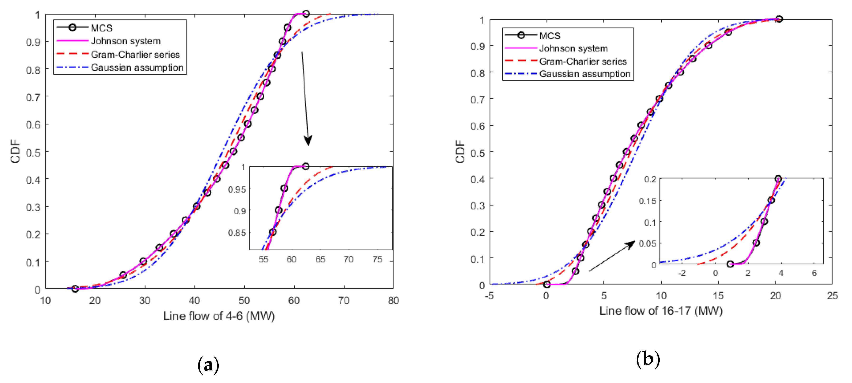
Figure 1. Cumulative distribution function (CDF) curve for line 4-6 flow (a) and line 16-17 flow (b).
Energies 13 02344 g001
Figure 2. Histograms of line flow 15–18 under preventive security-constrained optimal power flow (PSCOPF) (a) and chance-constrained PSCOPF (CC-PSCOPF) (b).
Energies 13 02344 g002
Figure 3. Generation cost (a) and violation probability (b) of CC-PSCOPF with different violation levels.
Energies 13 02344 g003
Table 1. The average root mean square (ARMS) value of evaluated methods.
LinesARMS of Cumulant + Johnson SystemARMS of Cumulant + Gram-CharlierARMS of Gaussian Assumption
Line 4–60.00310.12940.1312
Line 16–170.00380.12880.1306
Table 2. Generation Cost.
PSCOPFCC-PSCOPF
Cost ($/hr)7488.18196.5
Table 3. Constraint violation statistics.
PSCOPFCC-PSCOPF
Average violation probability0.00450.0010
Maximum violation probability0.07790.0100
N V 226
N a l v 1.951.5
N m l v 52
Table 4. Time consumption.
Test System PSCOPFCC-PSCOPF
IEEE-30Constraint Numbers160042
Time (s)1.230.13
IEEE-118Constraint Numbers33109187
Time (s)319.570.67