Abstract
This paper analyzes the drivers behind the changes of the Aggregate Carbon Intensity (ACI) of Latin America and the Caribbean (LAC) power sector in five periods between 1990 and 2017. Since 1990 the carbon intensity of the world has been reduced almost 8.8% whereas the carbon intensity of LAC countries only decreased 0.8%. Even though by 2017 the regional carbon intensity is very similar to the one observed by 1990, this index has showed high variability, mainly in the last three years when the ACI of LAC fell from 285 gCO2/kWh in 2015 to 257.7 gCO2/kWh. To understand what happened with the evolution of the carbon intensity in the region, in this paper a Logarithmic Mean Divisia for Index Decomposition Analysis (IDA-LMDI) is carried out to identify the accelerating and attenuating drivers of the ACI behavior along five periods. The proposal outperforms existing studies previously applied to LAC based upon a single period of analysis. Key contributions are introduced by considering the type of fuel used in power plants as well as specific time-series of energy flows and CO2 emissions by country. Results reveal structural reasons for the increase of the ACI in 1995–2003 and 2008–2015, and intensity reasons for the decrease of the ACI in 1990–1995, 2003–2008 and 2015–2017.
1. Introduction
Scientific research has found evidences that in the last two centuries, greenhouse gas (GHG) concentrations in the atmosphere are rising sharply. Carbon dioxide (CO2) concentrations reached 405.5 ppm in 2017, 146% of the pre-industrial era [1]. The Intergovernmental Panel on Climate Change (IPCC) is warning about the need to reduce anthropogenic GHG emissions to avoid a rise in global temperatures during this century [2].
The main source behind the increase in carbon dioxide concentrations is the increasing use of fossil fuels in power plants. For example, electricity-related emissions rose from 30.1% (6.25 of 20.51 GtCO2) by 1990 to 38.4% (12.5 of 32.8 GtCO2) by 2017 [3] and it is estimated to increase to 43% (18.7 of 43.7 GtCO2) by 2040 [4]. In 2017, Latin America and the Caribbean (LAC) countries CO2 emissions reached 1596 MtCO2 (one million tons of CO2) representing 4.8% of world energy-related emissions. Slightly more than 26% (416 Mt of 1596 MtCO2) of regional energy-related emissions are attributable to the combustion of fossil fuels in power generation plants. Despite this share seems low in an account of a high proportion of renewables in the regional generation energy matrix, the population increase, robust economic growth and the lack of new large-scale generation projects based in renewables are boosting investments on fossil-based electricity generation, mainly in Brazil. For this reason, the adequate identification of the key technical factors that explain the evolution of CO2 emissions in the LAC’s electricity sector is crucial in the context of new energy policies to be applied in the near future to contribute with the global mitigation strategy.
The changes of CO2 emissions of LAC countries are strongly correlated with increasing electricity demands [5]. For this reason, carbon emissions cannot be analyzed as a single magnitude but scaling by the unit of energy generated to take into account the relative size of each country. To do so, the Aggregate Carbon Intensity (ACI) is a performance indicator useful to characterize the behavior of the electricity sector from an environmental point of view [6,7]. The ACI indicator determines the relationship between the carbon dioxide emitted by fossil-fired power plants and the whole power generation system. The numerator represents the CO2 emissions from fossil fuels consumed for thermal generators, while the denominator represents the total electricity generated, coming from all sources. As a result, the ACI allows us to withdraw the effect of the underlying growth in demand and can vary across LAC countries. The units of the ACI indicator are generally expressed in grams of CO2 per each kWh produced. Figure 1 displays the evolution of the electricity-related carbon intensity in LAC countries and the world between 1990 and 2017 [3].
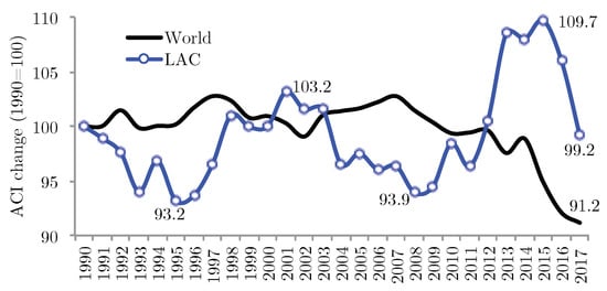
Figure 1.
Change of power sector’s aggregate carbon intensity in Latin America and the Caribbean (LAC) and the World, period 1990–2017, (1990 = 100) [3].
Notice that since 1990, the aggregate carbon intensity of the World has dropped about 8.8%. Instead, the ACI of LAC countries are showing a small decrease of 0.8%. We must highlight that the regional ACI index has showed high variability as can be observed in Figure 1, mainly in the last three years when the indicator fell from 285 gCO2/kWh in 2015 to 257.7 gCO2/kWh. This changing trend justifies focusing on the LAC electricity sector as it is expected to be an important contributor to the mitigation effort due to its large renewable resources.
Logarithmic Mean Divisia for Index Decomposition Analysis (IDA-LMDI) is a statistical decomposition procedure widely applied in the literature to analyze total carbon dioxide emission time-series [8]. A detailed review of applications on IDA-LMDI CO2 emission decomposition can be found in [9]. A comprehensive review of recent publications that use IDA to study CO2 emissions of the electricity sector is provided by [10]. IDA-LMDI analyses have been also applied in the U.S [11], China [12], the European Union [13], Philippine [14] and Greece [15] electricity generation sectors. However, we can observe that the vast majority of existing contributions are devoted to analyze carbon dioxide time-series. Few contributions are devoted to analyze ACI time series using statistical decomposition techniques. We would like to emphasize that carbon dioxide magnitudes in million tons of CO2 and carbon dioxide intensities in gCO2/kWh are different concepts. The ACI concept integrates both CO2 and power output magnitudes. This aspect is important in countries with high population growth such as LAC region. Further discussion about the key differences between both concepts are provided in [6]. For this reason, adequate analysis of ACI time-series in developing countries with increasing energy needs is necessary.
The IDA-LMDI procedures applied to ACI decomposition are scarce in literature as shown in Table 1. The methodology is general and it can be applied for any country or region of the world using either a single-period or a multi-temporal scope. Existing contributions on IDA-LMDI decomposition of ACI time-series are based on a single period, e.g., 1990–2017. Some examples are [6,16], for World and Asean carbon intensity time-series in 1990–2012 and 1990–2013, respectively. The carbon intensity of China’s power sector has been analyzed in [17,18,19] in the period 1990–2015. Recently, [7] analyzed the effect of the generation system capacity factor LAC’s power sector using a LMDI formulation considering a single period (1990–2015).

Table 1.
Contributions on carbon emission Logarithmic Mean Divisia for Index Decomposition Analysis (IDA-LMDI) analysis.
The main drawback of the single-period approach is that the drivers behind ACI variability are difficult to capture. Under a multi-temporal decomposition approach different accelerating and attenuating drivers of the ACI behavior can be analyzed in time-series with high variability, as the case of LAC’s ACI showed in Figure 1. As seen in Table 1, the multi-period IDA-LMDI approach has not been studied in LAC yet. To fulfill the research gap, this paper applies a multi-period IDA-LMDI method to determine the key factors that explain the changes of ACI in LAC’s power sector.
2. Aggregated CO2 Emission Intensities in LAC Countries
The estimated levels of carbon dioxide emissions associated with the power sector are different in each country of the region. The changes in the ACI between 1990 and 2017 by each country are presented in Figure 2. This figure shows the most representative countries. The remaining countries of the LAC region are grouped as the “rest of LAC countries” (ROLACs). It is observed that larger electricity producers as Brazil, Ecuador, Peru and Bolivia have significantly increased their carbon intensity between 1990 and 2017 but below the regional average by 2017 (257.7 gCO2/kWh). Other important producers as Mexico, Argentina, Chile, Colombia have reduced their carbon intensity concerning the average values. Notice that by 2017 countries such as Honduras, Guatemala and Haiti are showing important increases in their carbon intensity with respect to the ones observed in 1990.
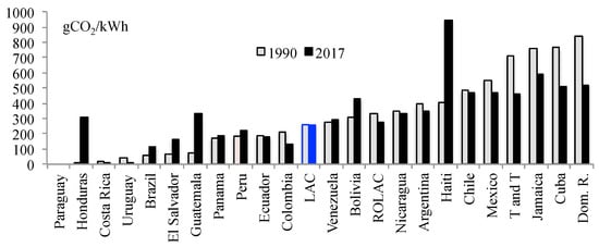
Figure 2.
The aggregate carbon intensity by LAC country, 1990–2017.
Brazil is the largest electricity producer of the region. The Brazilian ACI increased from 55 gCO2/kWh in 1990 to 113 gCO2/kWh in 2017. It is worth to mention that both figures are moderate with respect to the average values of LAC in 1990 (259.8 gCO2/kWh) and 2017 (257.7 gCO2/kWh), shown as blue bars in Figure 2. Mexico is the second electricity producer of the region. In this case, the carbon intensity fell from 549 gCO2/kWh in 1990 to 471 gCO2/kWh in 2017. The ACI of Mexico exceed the average values in both years. Most relevant reductions are achieved in Colombia, Uruguay and some Caribbean islands as Cuba, Jamaica, Trinidad and Tobago and the Dominican Republic. Argentina, Venezuela, Cuba and Nicaragua remains stable and as Paraguay has 100% renewable power sector, no emissions are assigned to this country.
To account for the impact of all countries electricity production levels, the carbon intensity figures depicted in Figure 2 for 1990 and 2017 are resettled in descending order and plotted against the cumulative electricity production. This exercise was previously performed by [6] using world carbon intensity evolution from 1990 to 2014. The resulting chart for the LAC case is depicted in Figure 3.
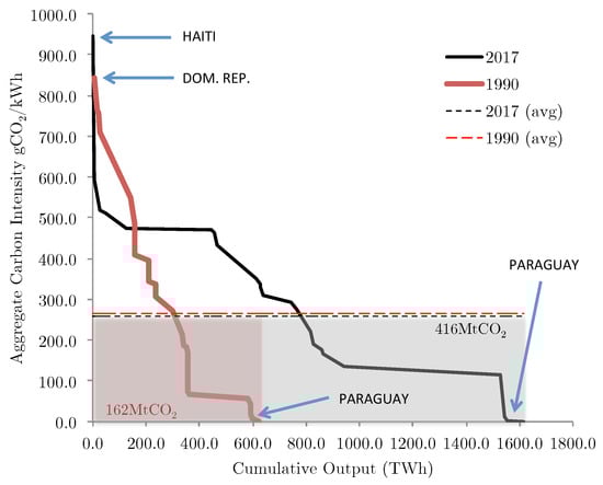
Figure 3.
Carbon intensity vs. cumulative electricity production in LAC, 1990–2017.
The cumulative curves of electricity output against ACI in each country are depicted as solid lines with different colors, red for 1990 and black for 2017, respectively [6]. The cumulative curve extends further to the right on the horizontal axis since total power output of 2017 was approximately three times the level registered in 1990. Note that the highest ACI observed corresponds to Dominican Republic (844 kgCO2/kWh in 1990) and Haiti (947 kgCO2/kWh in 2017). On the other hand, Paraguay showed zero power-related emissions in 1990 and 2017.
The area below both cumulative curves—represented by the two shadowed rectangles with 162 and 416 MtCO2, respectively—accounts the total CO2 emissions produced by all fuel-fired plants of LAC countries in 1990 and 2017. The 1990 and 2017 total average carbon intensity changed from 259.8 to 257.7 gCO2/kWh being represented by two horizontal dashed lines. Note that the range of the carbon intensity values in the vertical axis is almost the same for both years. As a matter of fact, the 2017 ACI average line overlaps the 1990 ACI average line. The difference between the ACI in 1990 and the ACI in 2017 is barely −0.8%.
Figure 4 shows how the regional carbon intensity 1990–2017. Note that over 28 years, five different accelerating and attenuating periods can be identified. Two increasing periods (1995–2003, 2008–2015) and three declining periods (1990–1995, 2003–2008, 2015–2017). In a previous work, [7] applied a LMDI analysis to the LAC’s ACI time-series (1990–2015) under a single-period basis. However, this approach does not capture the reasons behind the high variability observed during the whole period. It is necessary to apply a multi-period analysis in order to identify the role of each country in the ACI change in each period. In this paper, we apply the IDA-LMDI method under a multi-period basis to address this question. Next section provides the methodology and the assumptions made to select the length of each period.
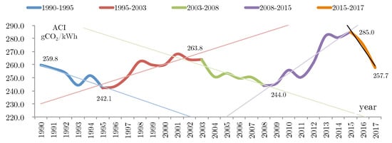
Figure 4.
The aggregate carbon intensity of LAC countries, 1990–2017.
3. Methodology
Laspeyres Index and Divisia Index Decomposition procedures are frequently used to perform analytics in energy and environmental studies [8,9]. The decomposed driving factors are associated with certain variables that explain the evolution of a variable of interest, i.e., the aggregate carbon intensity. In their original formulation, the Laspeyres Index and Divisia methods produce a residual factor that is difficult to explain [8]. The IDA-LMDI method proposed by [8] eliminates the residual term using a perfect decomposition.
In a specific year, Equation (1) expresses the total annual CO2 emissions from electricity as function of six series of variables (input time-series) [6].
where:
- n is the size of the dataset, the number of countries to considered in the analysis.
- i denoted the fossil fuel type. Three (f = 3) fuels are considered: coal (i = 1), natural gas (i = 2) and liquids from oil production (i = 3).
- is the power-related carbon dioxide emissions from fossil fuel i in a given countryj [ktCO2].
- is the total power-related carbon dioxide emissions from all fossil fuels in a given countryj [ktCO2]. Observe that .
- is energy input using fossil fuel type i in a given countryj [TWh].
- is the power output using fossil fuel type i in a given countryj [TWh].
- is the total power output from all fossil fuels in a given countryj [TWh]. Notice that .
- is the total power output (including renewable sources) in a given countryj [TWh]. Note that .
Three decomposition properties can be identified in the IDA Equation (1): (a) the total electricity output G is the main “activity” that produces CO2 emissions, (b) proportions , and indicate “structural” factors related with the share of the different fuel types in the fossil-based electricity mix of a given country j, the share of fossil-based production in the national electricity production and the share of national production concerning the total electricity output, (c) proportions and provide information about the “intensity” of each fuel type in local emissions and the efficiency of each generating plant fuel type, respectively. As made in the basic approach, total CO2 emissions should be normalized for kWh produced to obtain the ACI index, then Equation (1) can be rewritten as [6]:
where the following driving factors are defined:
- is the CO2 emission factor associated with fuel i in a given country j.
- is the heat rate of fossil-fired plants using fossil fuel type i in a given country j.
- is the proportion of power output from fossil fuel i in a given country j.
- is the proportion of power output from fossil fuels with respect to total power production in a given country j.
- is the power output in a given country j as a portion of total regional power output.
Equation (2) is then characterized by five factors, two structural factors ( = ) and three intensity factors (). Then and denote the structural and intensity drivers, respectively.
The IDA-LMDI method can be applied to two different scopes: additive and multiplicative decomposition formulation [7,9]. Both methods provide the same insight about the impact or effect of each driving factor at a given time frame. Both approaches are equivalent. In this paper, for the sake of simplicity, only the IDA-LMDI additive approach is considered. Additional considerations are provided for the selection of the extent and number of periods to be included under the multi-period approach.
The additive IDA-LMDI approach accounts the arithmetic change in total ACI from year to year as follows [6,7]:
where , , , and reproduce the effects between from and times associated with variations in , , , and , respectively.
Each effect of Equation (3) is interpreted as follows. The factor denotes the “CO2 intensity of the fuel-mix effect” expressing the changes in the emission factors applied to fossil fuels. The factor denotes the “generation efficiency effect” expressing the changes in power plant efficiency. The factor denotes the “fossil-share of electricity effect” expressing the changes in the share of fossil-based power output. The “fossil fuel-mix effect” that expresses the changes in the mix of fossil fuels used to produce fossil-based electricity (share of fossil-based electricity). The “geographical shift effect” that expresses changes in power output for a specific country with respect to regional power output.
Furthermore, the “intensity effect” and the “structural effect” encompass the impact of the fuel-mix ( = ) and the fossil-share ( = ), respectively. The detailed decomposition IDA-LMDI formulation used in this paper is included in the Appendix A [6,7].
The selection of final () and initial () times for each period is crucial to provide an adequate interpretation of the driven factors and their links with national energy policies. We argue that the length of each period must be enclosed into a given trend in the ACI time-series. Further research efforts must be carried out to define the number and extent of each period in the multi-period IDA-LMDI analysis.
In this paper we applied a qualitative approach to define the number and the extent of the periods to be used in the multi-period IDA-LMDI analysis. Some milestones related to the LAC countries and world energy economy are used as reference. From Figure 4 we identified five relevant periods: 1990–1995, 1995–2003, 2003-2008, 2008–2015, 2015–2017:
- Period 1990–1995: First ACI declining period. Institutional reforms in the LAC’s power sector are carried out. Many countries introduced market-oriented reforms in order to reduce electricity marginal prices. By 1995 the majority of LAC countries adopted any form of regulatory board for electricity. In this period oil prices showed a climbing trend reaching a local maximum in 1995.
- Period 1995–2003: First ACI increasing period. This period is characterized by lower oil prices. The Iraq conflict in 2003 represents the turning point in energy prices. During this period, all institutional reforms in the LAC’s power sector reach certain maturity. Some exceptions are Venezuelan and Mexican power sectors were no reforms were carried out. Phenomenon of “El Niño” in 2003.
- Period 2003-2008: Second ACI declining period. Rising oil prices period. As a result of global financial crisis in 2007 the oil prices plummeted drastically 2008. Phenomenon of “El Niño” in 2010.
- Period 2008–2015: Second ACI increasing period. Oil market price recovery period. Robust economic growth in the LAC region. Fracking techniques to produce shale gas and shale oil in the U.S. become widespread.
- Period 2015–2017: Third ACI declining period. In fall 2014 oil prices were reduced 50%. Phenomenon of “El Niño” in 2016.
Notice that we use 1990 as the initial year because, as a result of Kyoto, the majority of LAC countries initiated to account carbon dioxide emission magnitudes. The last year with available data is 2017.
Data sources and assumptions: Energy-related time-series of 22 countries that contribute most to the region’s CO2 emissions are considered. The remaining countries are grouped together as a single entity referred to as the “rest of LAC countries” (ROLACs) [7]. The energy and environmental dataset of j = 1, ..., 23 countries are taken from the IEA’s world energy model [20] whose energy balances are visible in the internet public database: https://www.iea.org/data-and-statistics/data-tables. The last year available is 2017. Four time series 1990–2017 are required to apply the methodology: , , , .
4. Results and Analysis
The additive IDA-LMDI method described in Section 3 has been applied to LAC countries using a multi-period approach.
In addition to the decomposition analysis for the main period 1990–2017, as a key contribution of this paper, the decomposition method has been applied under a multi-temporal basis considering five periods defined from Figure 4 as follows:
- 1990–1995 when the ACI changed (decreased) from 259.8 to 242.1 gCO2/kWh
- 1995–2003 when the ACI changed (increased) from 242.1 to 263.8 gCO2/kWh
- 2003–2008 when the ACI changed (decreased) from 263.8 to 244.0 gCO2/kWh
- 2008–2015 when the ACI changed (increased) from 244.0 to 286.0 gCO2/kWh
- 2015–2017 when the ACI changed (decreased) from 286.0 to 257.7 gCO2/kWh
The interested reader can replicate the results reported in this section by assessing the following GitHub web page https://github.com/pmdeoliveiradejesus/LMDI-LatinAmerica/.
The additive decomposition method is applied according to Equation (3), and using Equations (A1)–(A5) of the Appendix A. General results over the main period 1990–2017 and for the five periods (1990–1995, 1995–2003, 2003–2008, 2008–2015 and 2015–2017) are presented in Table 2. All figures of the table are given in gCO2/kWh.
Table 2.
Additive IDA-LMDI analysis results (gCO2/kWh).
The first column of Table 2 lists the periods of study. The second column includes the total changes of ACI () for each period. The overall ACI change between 1990–2017 is = −2.15 gCO2/kWh (0.8%, highlighted in green color). The next two columns in the table account the structural and intensity effects ( and ) for each period. The structural driver corresponds to the sum of the fuel-share in the electricity output and the geographical shift effects ( = + ). The intensity driver corresponds to the sum of the emission, efficiency and fuel-mix effects ( = + + ). The intensity driver associated with the carbon emission intensity () and efficiency () as well as the structural effect associated with fuel-share of electricity () were also decomposed by fuel type and presented in Table 3.
Table 3.
The additive IDA-LMDI analysis results by fuel type in all periods (gCO2/kWh).
Some additional notation is necessary to highlight the results enclosed in Table 2 and Table 3. To indicate the most important effects that contribute to the actual trend of the ACI table entries are highlighted in bold blue. Conversely, the most important effects that do not contribute (mitigate) to actual trends are highlighted in bold red. In addition, Figure 5 displays a graph representation of results presented in Table 2. The solid circles depicted in Figure 5 over each period bar representation also indicate the total ACI changes ().
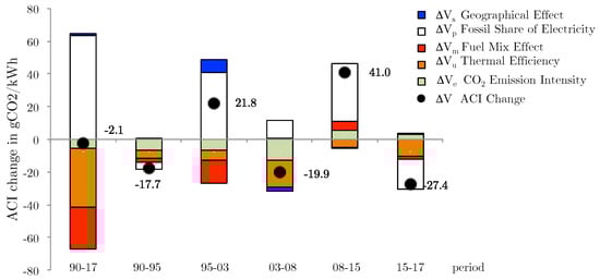
Figure 5.
Additive IDA-LMDI analysis considering five periods (gCO2/kWh).
It is possible to observe the following general results in each period:
- 1990–2017 the ACI changed (decreased) from 259.8 to 257.7 gCO2/kWh due to INTENSITY reasons (improvements in gas-fired plant efficiency).
- 1990–1995 the ACI changed (decreased) from 259.8 to 242.1 gCO2/kWh due to INTENSITY reasons (improvements in fuel-fired plant efficiency).
- 1995–2003 the ACI changed (increased) from 242.1 to 263.8 gCO2/kWh due to STRUCTURAL reasons (fossil-share increase)
- 2003–2008 the ACI changed (decreased) from 263.8 to 244.0 gCO2/kWh due to INTENSITY reasons (improvements in coal-fired plant efficiency).
- 2008–2015 the ACI changed (increased) from 244.0 to 286.0 gCO2/kWh due to STRUCTURAL reasons (fossil-share increase)
- 2015–2017 when the ACI changed (decreased) from 286.0 to 257.7 gCO2/kWh due to INTENSITY reasons (improvements in coal-fired plant efficiency and decrease of fossil-share).
In the following, we will analyze these overall results considering the intensity and structural drivers obtained by country.
4.1. Period 1990–2017
Specific results of intensity and structural drivers by country for the main period 1990–2017 are presented in Table 4.
Table 4.
Additive IDA-LMDI analysis by country 1990–2017.
A remarkable mitigating effect on the ACI change between 1990–2017 is attributable to Cuba and Mexico: = −11.9 gCO2/kWh and = −8.0 gCO2/kWh. The most important accelerating effect on the ACI change between 1990–2017 is regarded as being caused by Brazil: = −+21.8 gCO2/kWh.
Figure 6 shows the contribution of all LAC countries from intensity and structural views. From the intensity viewpoint, in general, all LAC countries become less intense (almost all intensity drivers are negative). This implies an overall improvement on efficiency and fuel-mix strongly linked to more efficient electricity markets. Best improvements in efficiency and a more decarbonized fuel-mix are observed in Mexico, Brazil and Argentina. On the other hand, about the structural viewpoint, Brazil is showing the most important fossil-share of the region. However, it is worth to mention that structural effect has two components: fossil-share and geographical shift effects. As seen in Table 4 the geographical effect is negligible = 1.58. Some countries such as Venezuela and Chile are showing important differences.
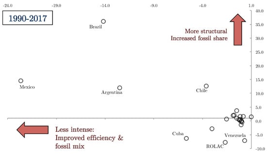
Figure 6.
Structural and intensity effects by country, period 1990–2017.
In particular, results shown in Table 4 permit to evaluate the evolution of each country by effect: (efficiency), (fossil-mix) and (fossil-share). For example, the driver (Equation (A4)) allow us to tackle the effect of the increase/decrease of the fossil-generation share upon the overall carbon intensity. In Table 4, seventh column, we observe how between 1990–2017 Brazil and Venezuela have increased the share of fossil-sources, contributing to boost overall ACI ( = 35 gCO2/kWh and = 1.2 gCO2/kWh). On the other hand, Colombia has lowered the fossil share with a mitigating impact on the overall ACI ( = −1.2 gCO2/kWh). This means that Brazilian power sector is going in the opposite direction of Colombian power sector from fossil-share effect viewpoint. Since 1990, Colombia shows a decarbonization process with a slight increase of renewable sources participation un the power dispatch. On the other hand Brazil has a decisive contribution on the ACI increase due to massive incorporation of gas-fired plants [21].
From the efficiency and fossil mix effect viewpoint, Argentina and Mexico are showing important improvements allowing significative reductions on overall ACI. Note from Table 4, fifth and sixth columns, that = −10.01 gCO2/kWh and = −13.94 gCO2/kWh are clearly the most important mitigating effects on overall regional ACI. In general all LAC countries have improved their fossil-mix and fossil-share effects. As a result, the intensity effect associated with efficiency and fuel-shift policies are explaining the reduction of 0.8% in the overall ACI since 1990, as shown in Figure 1.
4.2. Period 1990–1995
In the period 1990–1995, the ACI reduction observed (−6.9%) is described by changes in intensity ( = −14.1 gCO2/kWh), specifically due to the improvement of efficiency ( = −4.7 gCO2/kWh), mainly associated with integration of more efficient gas-fired plants ( = −4.7 gCO2/kWh) in Argentina. It is worth noting that structural drivers also explain the decrease of the ACI ( = −4.5 gCO2/kWh) due to the integration of large hydro resources in Venezuela. During this lapse, improvements, both in structure and intensity, were observed.
4.3. Period 1995–2003
In the period 1995–2003, the ACI increase observed (11.0%) is described by changes in structure ( = 48.6 gCO2/kWh), specifically due to an increased fossil-share of electricity output ( = 40.7 gCO2/kWh), mainly associated with integration of fossil fuel-fired plants in Mexico and Brazil.
4.4. Period 2003–2008
In the period 2003–2008, the ACI reduction observed (−9.1%) is explained by changes in intensity ( = −28.4 gCO2/kWh), specifically due to the improvement of efficiency ( = −16.0 gCO2/kWh), mainly associated with the modernization of fuel oil thermal plants ( = −9.2 gCO2/kWh) in Mexico.
4.5. Period 2008–2015
In the period 2008–2015, the ACI increase observed (17.1%) is described by changes in structure ( = 34.8 gCO2/kWh), specifically due to an increased fossil-share of electricity output ( = 35.4 gCO2/kWh). The main actor is Brazil with large integration of fossil fuel-fired plants.
4.6. Period 2015–2017
In the period 2015–2017, the ACI reduction observed (−9.9%) is described by changes in both intensity ( = −9.2 gCO2/kWh) and structure ( = −18.2 gCO2/kWh). Intensity effects were characterized by the improvement of efficiency ( = −10.6 gCO2/kWh) in Argentina and Brazil. It is worth to note that structural drivers also explain the decrease of the ACI ( = −18.4 gCO2/kWh) due to a decrease of the fossil share in Brazil. Figure 7 shows the changes of ACI total, intensity and structural by country for the period 2015–2017. The “El Niño” phenomenon in 2015–2016 affected hydroelectric production in the Andean countries.
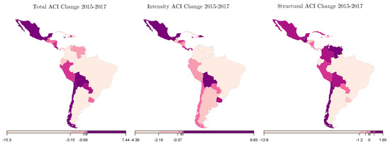
Figure 7.
LMDI analysis applied to emissions by country, period 2015–2017.
4.7. Perspectives for LAC’s Power Sector
The future evolution of future CO2 emissions might take different ways depending on the mitigation policy adopted in each country. Two future projections for LAC’s ACI are provided by the IEA. Under the New Policies Scenario (NPS), it is expected a reduction of 39% (from 286 gCO2/kWh in 2017 to 175 gCO2/kWh in 2040). Under the sustainable development scenario (450S) a strong decrease of 79% is also expected (from 286 gCO2/kWh in 1990 to 61 gCO2/kWh in 2040). Then, both scenarios are showing a clear declining trend. The historical trend observed in 2015–2017 is aligned with both future scenarios. However, the accomplishment of the sustainable development goal (61 gCO2/kWh in 2040) will require additional efforts from intensity and structural perspectives.
5. Conclusions
The aggregate carbon intensity (ACI) time-series registered in Latin America and the Caribbean countries from 1990 to 2017 can be divided in five different periods: two periods with an increasing trend and three periods with a declining trend in the ACI index. No previous studies analyzed the drivers that explain the ACI change of the region using a multi-period basis. The conclusions are the following:
- Period 1990–1995: the ACI decreased from 259.8 to 242.1 gCO2/kWh. Intensity drivers explain this decrease, mainly due to improvements in fuel-fired plant efficiencies in Argentina.
- Period 1995–2003: the ACI rose from 242.1 to 263.8 gCO2/kWh. Structural drivers explain this increase, mainly due to rising fossil-shares in Mexican power sector.
- Period 2003–2008: the ACI fell from 263.8 to 244.0 gCO2/kWh due to intensity effects, explained by improvements in existing coal-fired plant efficiencies in Mexico.
- Period 2008–2015: the ACI increased from 244.0 to 286.0 gCO2/kWh due to structural effects mainly in Brazil. Brazilian electricity market incorporated a large amount of fossil-based energy sources in this period.
- Period 2015–2017: the ACI decreased from 286.0 to 257.7 gCO2/kWh due to intensity reasons. No particular country’s power sector is explaining this change. In general, all LAC countries have improved efficiency and fuel-mix in their fuel-fired power plants. The “Niño” phenomenon in 2015-2016 affected hydroelectric production.
The latter result has important political implications, since the current declining trend (reaching 257.7 gCO2/kWh in the last three years) is aligned with the sustainable development scenario. However, the goal is quite far: 62 gCO2/kWh by 2040. For this reason, Brazil’s future energy policy and the constitution of an Andean electricity market will be crucial to achieve the climate change objectives of LAC countries.
In this paper we applied a standard decomposition method to determine the driving factors behind the changes in the LAC’s ACI indicator. These drivers are of technical nature: efficiency, fossil share, etc. However, other indirect explanatory factors such as population, gross domestic product, oil prices and investment flows must be included. Available socioeconomic and technical time-series show several correlation problems. The adoption of Bayesian models to evaluate the ACI evolution deserves attention in future research.
Author Contributions
Conceptualization, P.M.D.O.-D.J.; Investigation, P.M.D.O.-D.J., J.J.G. and D.R.-L.; Methodology, P.M.D.O.-D.J., J.J.G. and D.R.-L.; Validation, J.M.Y.; Writing – original draft, P.M.D.O.-D.J. and D.R.-L.; Writing – review & editing, P.M.D.O.-D.J. and J.M.Y. All authors have read and agreed to the published version of the manuscript.
Funding
This research received no external funding.
Conflicts of Interest
The authors declare no conflict of interest.
Appendix A. Decomposition IDA-LMDI Formulae for the Additive Approach
The decomposition IDA-LMDI formulae for the additive approach is included below:
where , and
References
- World Meteorological Organization. WMO Greenhouse Gas Bulletin (GHG Bulletin)- No. 14: The State of Greenhouse Gases in the Atmosphere Based on Global Observations through 2017. 2017. Available online: https://library.wmo.int/ (accessed on 15 January 2020).
- Intergovernmental Panel on Climate Change. Climate Change 2007 Synthesis Report. Technical Report Contribution of Working Groups I, II and III to the Fourth Assessment Report of the Intergovernmental Panel on Climate Change; IPCC: Geneva, Switzerland, 2007.
- CO2 Emissions from Fuel Combustion; International Energy Agency: Paris, France, 2019.
- World Energy Investment Outlook; International Energy Agency: Paris, France, 2014.
- Román, R.; Morales, V. Towards a sustainable growth in Latin America: A multiregional spatial decomposition analysis of the driving forces behind CO2 emissions changes. Energy Policy 2018, 115, 273–280. [Google Scholar] [CrossRef]
- Ang, B.W.; Su, B. Carbon emission intensity in electricity production: A global analysis. Energy Policy 2016, 94, 56–63. [Google Scholar] [CrossRef]
- De Oliveira De Jesus, P. Effect of generation capacity factors on carbon emission intensity of electricity of Latin America and the Caribbean, a temporal ida-lmdi analysis. Renew. Sustain. Energy Rev. 2019, 101, 516–526. [Google Scholar] [CrossRef]
- Ang, B.W.; Liu, F.L.; Chew, E.P. Perfect decomposition techniques in energy and environmental analysis. Energy Policy 2003, 31, 1561–1566. [Google Scholar] [CrossRef]
- Ang, B.W.; Zhang, F.Q. A survey of index decomposition analysis in energy and environmental studies. Energy 2000, 25, 1149–1176. [Google Scholar] [CrossRef]
- Xu, X.Y.; Ang, B.W. Index decomposition analysis applied to CO2 emission studies. Ecol. Econ. 2013, 93, 313–329. [Google Scholar] [CrossRef]
- Jiang, X.T.; Li, R. Decoupling and Decomposition Analysis of Carbon Emissions from Electric Output in the United States. Sustainability 2017, 9, 886. [Google Scholar] [CrossRef]
- Zhao, Y.; Li, H.; Zhang, Z.; Zhang, Y.; Wang, S.; Liu, Y. Decomposition and scenario analysis of CO2 emissions in China’s power industry: Based on LMDI method. Nat. Hazards 2017, 86, 645–668. [Google Scholar] [CrossRef]
- Karmellos, M.; Kopidou, D.; Diakoulaki, D. A decomposition analysis of the driving factors of CO2 (Carbon dioxide) emissions from the power sector in the European Union countries. Energy 2016, 94, 680–692. [Google Scholar] [CrossRef]
- Sumabat, A.K.; Lopez, N.S.; Yu, K.D.; Hao, H.; Li, R.; Geng, Y.; Chiu, A.S. Decomposition analysis of Philippine CO2 emissions from fuel combustion and electricity generation. Appl. Energy 2016, 164, 795–804. [Google Scholar] [CrossRef]
- Diakoulaki, D.; Giannakopoulos, D.; Karellas, S. The driving factors of CO2 emissions from electricity generation in Greece: An index decomposition analysis. Int. J. Glob. Warm. 2017, 13, 382–397. [Google Scholar] [CrossRef]
- Ang, B.W.; Goh, T. Carbon intensity of electricity in ASEAN: Drivers, performance and outlook. Energy Policy 2016, 98, 170–179. [Google Scholar] [CrossRef]
- Peng, X.; Tao, X. Decomposition of carbon intensity in electricity production: Technological innovation and structural adjustment in china’s power sector. J. Clean. Prod. 2018, 172, 805–818. [Google Scholar] [CrossRef]
- Liu, N.; Ma, Z.; Kang, J. A regional analysis of carbon intensities of electricity generation in China. Energy Econ. 2017, 67, 268–277. [Google Scholar] [CrossRef]
- Liu, N.; Ma, Z.; Kang, J.; Su, B. A multi-region multi-sector decomposition and attribution analysis of aggregate carbon intensity in china from 2000 to 2015. Energy Policy 2019, 129, 410–421. [Google Scholar] [CrossRef]
- IEA. World Energy Model; IEA: Paris, France, 2019. Available online: https://www.iea.org/reports/world-energy-model (accessed on 15 December 2019).
- Ministry of Mines and Energy of Brazil (MME). Electricity in the 2024 Brazilian Energy Plan (PDE 2024). Available online: http://www.mme.gov.br/ (accessed on 17 January 2020).


© 2020 by the authors. Licensee MDPI, Basel, Switzerland. This article is an open access article distributed under the terms and conditions of the Creative Commons Attribution (CC BY) license (http://creativecommons.org/licenses/by/4.0/).