Abstract
The Gordon-Ng models are tools that have been used to estimate and evaluate the performance of various types of chillers for several years. A 550 TR centrifugal chiller plant facility was available to collect data from July and September 2018. The authors propose rearranging variables of the traditional (GNU) model based on average electric consumption and through a thermodynamic analysis comparable to the original model. Furthermore, assumptions are validated. Then, by estimation of the parameters of the new model using least square fitting with field training data and comparing to the GNU model and Braun model (based on consumption), it was shown that the proposed model provides a better prediction in order to evaluate consumption of a centrifugal chiller in regular operation, by improving the coefficient of variation (CV), CV = 3.24% and R2 = 92.52% for a filtered sub-data. Through an algorithm built from steady-state cycle analysis, physical parameters (Sgen, Qleak,eq, R) were estimated to compare with the same parameters obtained by regression to check the influence of the interception term in the model. It was found that without an interception term, the estimated parameters achieve relative errors (ER) below 20%. Additional comparison between external and internal power prediction is shown, with CV = 3.57 % and mean relative error (MRE) of 2.7%, achieving better accuracy than GNU and Braun model.
1. Introduction
Nowadays, there is a great effort dedicated to improving heating, ventilation and air conditioning (HVAC) equipment efficiency, especially in chillers, which are equipment used extensively in buildings and industrial air conditioning installations. Therefore, it is crucial to evaluate their performance continually for optimization processes and failure prediction. This situation creates a necessity to generate more accurate models that allow simulation to predict their behavior. Traditionally, engineering models are classified into three categories: black-box, grey-box, and physical or mechanistic models [1,2,3,4,5]. These can be steady-state or dynamic models. The former has the disadvantage that only applies to the data range used to fit model parameters. The latter method needs exact information about the equipment geometry, materials, and data that usually only manufacturers can provide. That makes the analysis of a process very hard when it is not possible to obtain manufacturer data.
Many authors have made several thermodynamic models for chillers. One of the first research in the performance evaluation of a centrifugal chiller was carried out by Braun [6], who proposed a new empirical model based on consumption as a quadratic function. Subsequently, Gordon et al. developed semi-empirical thermodynamic models [7,8,9] based on easily measurable variables for reciprocating, centrifugal and absorption chillers. This model is known as the universal model (GNS) in which the parameters are inherent to each type of compressor [7]. Later, a work developed by Ng et al. [8,9] for reciprocating chillers resulted in the fundamental model (GNU). These Gordon–Ng models are useful for optimization, prediction, and diagnosis of chillers.
Lee [3,10] proposed a model similar to GNU with a modification applied to screw chillers with experimental validation and good accuracy, but the model was not on centrifugal chillers. Indeed, after the development of Gordon–Ng models, there has been no other registered different semiempirical model for centrifugal chillers. Browne and Bansal [11] investigated steady-state physical models applied to centrifugal liquid chillers, although they had the disadvantage mentioned above: they needed some physical information to describe the compressor adequately. Also, steady states models are not robust enough for prediction of performance under different load conditions, variable flowrate, or variable speed drives. Several comparisons have been taken to attain empirical and semi-empirical models [12,13,14]. Jiang and Reddy [4,5,15,16] proposed a new reevaluation and modification of the Gordon–Ng model (GNU), based on the fact that this model applies to inlet guide vane control (IVC) chillers, without variable speed control. The authors concluded that the fundamental model could be applied under special specific conditions. Lee [10] evaluated six empirically based models testing in chillers under different conditions with better accuracy (CV < 1%) using the polynomial (MP) and the bi-quadratic (BQ) regression model.
Evaluating chiller performance is significant to yielding, reducing costs of operation and maintenance, failures, and monitoring time. It is necessary to predict the behavior of a chiller, but sometimes there is few available data. For this reason, there is a need for robust models. Saththasivan [17,18] tested the GNU model on a centrifugal chiller, finding that only partial diagnosis is possible. Recently, black-box models are commonly used for fault detection and diagnosis (FDD) purposes [19,20] through advanced statistical methods as Box-Cox regression, clustering, neural networks and others [19,21,22,23,24]. Although these models display high accuracy, their parameters have no physical meaning, which can be useful to performance and thermodynamic analysis by exploring the effect of a parameter linked to irreversibilities or geometrical properties, over the consumption or efficiency. Another issue is regarding the management of data and fitness of the model. Authors usually show metrics regard to the accuracy, but often some information about the utility of the model (testing assumptions) is missing. Some research in this area has been carried out by performing the traditional Least Squares as a regression method [15,25,26]. Recently, Acerbi (2019) found that there is no significant improvement when Non-Linear Square method is used instead of traditional.
Taking into account the above papers is worth developing some research about: (1) the validity of the GNU model in a centrifugal chiller with an improved control system to keep a stable operation if this model initially was built over some assumptions based on a reciprocating chiller; (2) Testing the suitability of the regression method; and (3) exploring the improvement of the GNU model by the modification of some variables. This paper aims to perform a rearranged Fundamental Gordon–Ng model, based on power consumption instead of COP (coefficient of performance). There are some benefits of this choice: first, COP is an indirectly measured variable that expresses an “automatic” state; meanwhile consumption is measured directly by the control system and denotes the input power measured in a period of time. Second, some research could be made in the future, analyzing the consumption when operational and geometric parameters change. On the other hand, the authors expect to do further work in the direction of a dynamic model, and any data-driven model can be necessary to calculate consumption without factory data. Besides a mathematical modelling of consumption is proposed to analyze the validity of the assumptions made to get the final model and physical parameters. There are two topics to evaluate:
- The accuracy of the parameters obtained by the regression model.
- The internal and external power prediction of the model.
Both results can be valuable tools to evaluate the performance of the centrifugal chiller and eventually fault detection.
The paper is organized as follows. The first part contains mathematical and thermodynamic derivation of the models, description of the facility equipment and datasets, and thermodynamic analysis to estimate physical parameters through an algorithm and assumptions of the GNU model. From the training data, physical parameters were obtained and compared, using the regression method (with and without an intercept term) and the algorithm. Also, the accuracy of the model was investigated and contrasted to fundamental GNU and Braun models through statistical metrics. The assumption of independence of residuals was checked. From the testing data, the accuracy and prediction capacity of the three models were compared over different sub-data chosen according to its setpoint supply temperature. Finally, some results and conclusions are discussed briefly.
1.1. Empirical and Semiempirical Models
Following the Ng–Gordon method, a chiller cycle is analyzed [7]. Figure 1 shows a simple-vapor-compression cycle for a conventional chiller plant in which all the measurable variables are shown. Some assumptions are required:
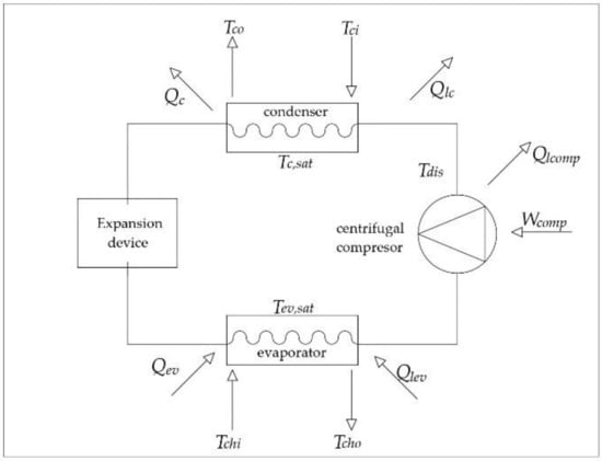
Figure 1.
Simple-vapor-compression cycle basic scheme.
- Steady state condition.
- Uniform Flow.
- Heat losses in the expansion device and pipe are negligible.
- Energy losses between electric motor and compressor are not considered.
- Water flow at the evaporator and condenser are constant.
- Water and refrigerant heat capacity (c) are constants.
- Tc,sat and Tev,sat are constants.
- Drop pressure in the heat exchangers, where no phase change along the process, is not considered.
- Superheating and subcooling neglected due to the lack of data.
A total heat loss term, QLT (kW), is defined in Figure 1. This term is calculated from Equation (1):
where Qlev (kW) is the heat losses at the evaporator, Qlc (kW) is the heat rejected at the condenser, and Qlcomp (kW) is the heat losses at the compressor. Using the First Law of Thermodynamics for the cycle:
Entropy net change for the chiller expresses as:
where (kW/K) is the irreversibility due to the entropy generated in the chiller, friction losses in the compressor, and the expansion device, the cooling load, Qev (kW), it is the heat or heat transfer rate removed from the building through water flow. It can be calculated in several ways. From the heat exchanger where inlet and outlet refrigerant temperatures and evaporator geometry must be known, and from thermal capacitance (Equation (4)) approach:
where is the thermal capacitance of cooling water (kW/K). With as mass flow rate (kg/s).
Similarly, for the removed heat in the condenser:
It is assumed, in Equation (3), that heat exchange through boundaries occurs at constant temperatures. It is, therefore, necessary that both temperatures are in terms of measurable variables.
To estimate those temperature, according to the ε-NTU method:
where defined as:
where
Due to overheating and subcooling being negligible, an isothermal process takes place in the evaporator and condenser. For the evaporator, the temperature can be expressed according to Equation (8):
Similarly, for the condenser:
With and
Replacing Equations (2), (8) and (9) in Equation (3):
Furthermore, rearranging this equation and expressed in terms of A, B, C, D, and E coefficients:
where,
According to Ng [8], these equations can be approximated based upon actual measured values for reciprocating chiller. There is no evidence in centrifugal chillers; for this reason, these terms will be estimated from real data. Due to evaporator and condenser are well insulated (pipe and shell heat exchangers), Qlc is negligible, and some terms related to the resistances (, ) are neglected because of their low values.
Replacing Equation (1) into Equation (17), an expression is obtained for the average heat losses from the evaporator and condenser to the ambient. Ng and Gordon [8] call this term
A Wcomp expression is obtained by simplifying Equation (11):
where,
Gordon’s model original parameters, in Equation (22), are maintained. But now the output variable is Wcomp. A fourth term is added. The expression can be rearranged to have the same parameter with physical meaning, Sgen, Qleak,eq and R:
Then, Equation (24) becomes:
where, , .
1.2. Fundamental Gordon-Ng Model
Gordon–Ng (GNU) is a simple thermodynamic model derived from the First and Second Laws of Thermodynamics. This model applies to all chiller types [9] and is based on the coefficient of performance (COP) as a linear function of refrigeration load and temperatures that easily measurables in a cooling plant. The model takes the following form:
where b1, b2 and b3 have physical meaning:
- b1 = Sgen = Internal entropy generation.
- b2 = Qleak,eq = Rate of heat losses or gains from the chiller.
- b3 = R = Total heat exchanger thermal resistance.
1.3. Biquadratic Braun Model
The model proposed by Braun is an empirical or black-box one, also called the biquadratic model. Predicts a standardized power consumption based on only two inputs with five coefficients and interception term (Equation (27):
where X = Q/Qdes and Qdes is designed cooling capacity of the chiller. Z0 is the designed input power of the chiller. As such,
2. Materials and Methods
The chiller plant operates at the Engineering Building at Universidad del Norte, Colombia, and manufactured by York® (OptiviewTM Software C.OPT.01.08A.300 version 10.0, Johnson Controls, PA, USA). The plant comprises one centrifugal chiller unit of 550 TR, four water-cooling towers, and a cold-water loop with constant primary water flow rate through the evaporator. The condenser circuit has constant-flowrate. The centrifugal chiller is a single-stage compressor type with prerotation vanes (PRV) for capacity control and a variable speed driver. A proprietary system, Metasys, manage inputs, and measured outputs. The chiller working fluid is R134a. Technical data can be seen in Table 1.

Table 1.
York® Centrifugal Chiller technical data.
The OptiViewTM York control center provides temperature and pressure data. Pressure transducers and thermistor with DC voltage as output mounted in various locations have different ranges. The uncertainties of the measured values are listed in Table 2. The data used for the model correspond to a stable state, with the restriction that the temperature values do not change above 1% during a time interval of 10 minutes. Table 2 shows the data intervals collected during July and September 2018. Data filtering was done as follows:
Table 2.
Range of values for data corresponding to a centrifugal chiller operation in July and September 2018.
- Wrong data due to sensor malfunction or system errors.
- Unusual data is rejected: negatives and zeros values and large power values.
- Cooling load percentage below 10% and above 100%.
- Values related to all aspects of the dynamic system: Powering up and down of equipment.
- Data, according to Standard AHRI 550/590 [27].
Original data was collected through de building automation system (BAS), corresponding to 4464 data points for July and 4320 for September. Both months have highly cooling load dynamics. September will be used to internal prediction and July for external prediction. Both data have been filtered for two ranges of outlet water chilled temperatures relatives to Standard rating Air conditioning, heating and refrigeration institute (AHRI) conditions between 4.4 °C and 8.9 °C. July has been averaged to build a load and consumption profile. Table 3 shows the number of data points for every group of data after filtering.
Table 3.
Data points used to internal and external prediction.
2.1. Estimation of Thermodynamic Parameters
Through a thermodynamic analysis, the b and c values for Equations (1) and (27) are calculated. The estimation of parameters is made as closely as possible of steady-state operation with data collected. Some assumptions must be included, even a superheating value (not allowable from data). This analysis requires next assumptions:
- Superheating: 5 °C.
- Throttling device is isenthalpic.
- Point 4′ in Figure 2 is saturated liquid at evaporator pressure.
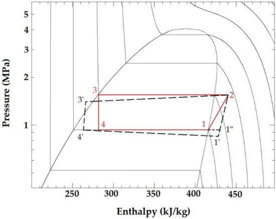 Figure 2. Pressure–enthalpy diagram for vapor compression cycle with R134a.
 - Point 2 (discharge temperature is at condenser pressure).
- Pressure drop by inlet guide vanes is negligible.
- Constant water flow rate through the condenser.
Figure 2 is a schematic pressure–enthalpy diagram for operating conditions of a vapor compression cycle. System BAS can provide saturation temperatures and nominal pressures relatives to points 1 to 4. The red line corresponds to an ideal isentropic cycle and dashed line to real operating points.
From First Law of Thermodynamics applied to evaporator, condenser, and compressor, the following expressions have been obtained:
Also, Qc from Equation (6):
Based on next assumptions:
- Enthalpy at superheating temperature at evaporator pressure.
- Enthalpy of saturated liquid at condenser saturated temperature.
- Assuming isenthalpic-throttling device.
- Enthalpy of overheated vapor at discharge temperature and condenser pressure.
As is unknown, an algorithm to determinate Qlev, Qlc, Qlcomp, and converging from a seed value is developed. Parameters Qleak,eq, R, and Sgen can be calculated from Equations (21), (23), and (3). The flow chart of the algorithm is shown in Figure 3. This program fastening calculates properties in different states from temperature and pressure data. Then, from the energy balances compute the heat leaks, loads, and consumption, through an iterative cycle assuming an initial value of refrigerant flow mass for residual convergence of 10−5. Finally, estimates parameters set by the below Equations and Formulas (31) and (32).
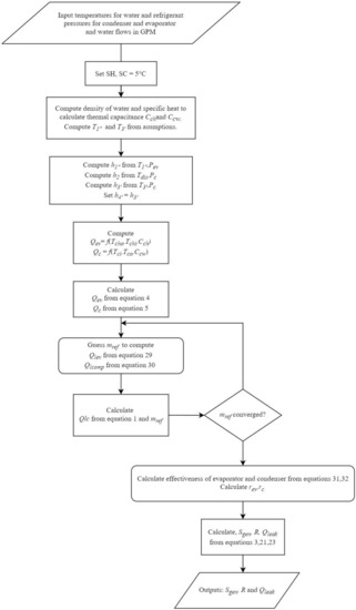
Figure 3.
Flowchart of the algorithm to estimate parameters of the chiller.
Effectiveness from Equation (6) can be expressed for both heat exchangers, as:
2.2. Regressor Parameters Estimation
Regressor parameters from Equations (24) and (26) can be estimated by regression analysis. Although some authors have studied the use of Time series or Non-linear regression [15,25], in the first case, there is no enough data by year to analyze a seasonal behavior; in the second case, the author concluded that there is not a significant practical improvement by using a Non-linear procedure. It should have been noted that both Equations ((24), (26)) are implicit, so the response variables (Wcomp, COP) are not corresponding to the response model variable y. In order to estimate physical parameters with moderate computational effort, an Ordinary Least Squares method has been used.
On the other hand, there is a discussion about the inclusion of the interception term. Reddy recommends using an interception purely for prediction purposes and not to use it for estimate parameters [4]. In order to investigate it, GNU and GNU rearranged models have been fitted in two manners, one corresponding to Equation (25), and another one including the interception term:
Equation (25) is regressed for both models to estimate physical parameters and compare them with parameters obtained by thermodynamic analysis. Then, Equation (33) is regressed for both models to evaluate internal and external predictions. Next metrics have been used to compare:
The square correlation coefficient R2 and R2adjusted:
where ymi is the modeling (or predicted) value, and yei is the experimental value of the i-th data, n is the number of data points and p the number of parameters to be regressed.
The mean relative error (MRE) and the relative error (RE) for parameters:
The predictive accuracy can be assessed considering the coefficient of variation (CV) of the root mean squared error (RMSE), which indicates how well the model satisfies the predictions.
3. Results and Discussion
From the September data, a profile can be built to assess the chiller behavior and contrast it with thermodynamic analysis. Three variables are evaluated: cooling load (calculated with Equation (5)), coefficient of performance (COP), and the consumption per cooling load (In TR). The September profile is depicted in Figure 4. Note that it seems to be two regimes of load, close to 0.2 and close to 0.7. A histogram (Figure 5) shows this behavior and essential information about the distribution of data for model assumptions. There is a normal distribution biased to the left relative to points of low cooling load.
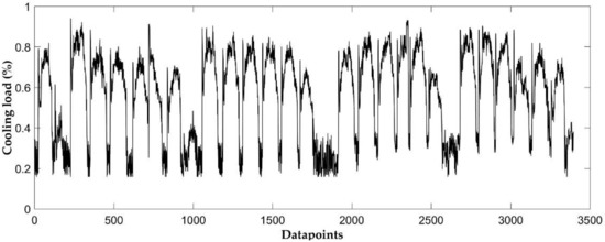
Figure 4.
Load profile for September 2018.
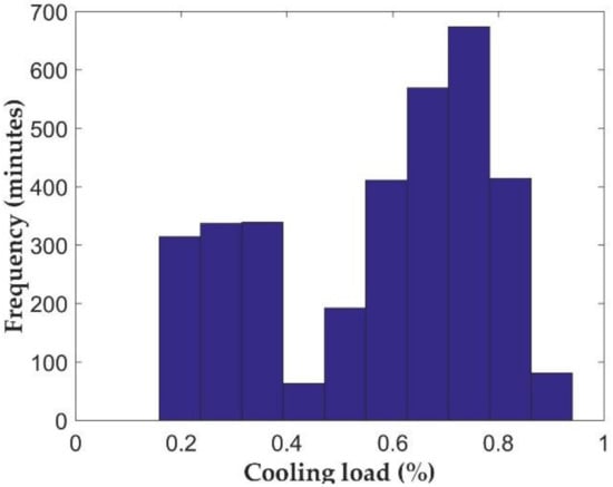
Figure 5.
Histogram to observe the distribution of data regarding the regime of cooling load.
In order to assess the behavior of performance and efficiency according to cooling load regimes, it should be added an efficiency profile (in kW per TR) to load profile for a sub-data of September. Figure 6 shows a recurrent profile per day; at the beginning and the end of the day, the chiller operation is at low load, but most of the daily operation is at partial load, approximately 80% of the design load which is a typical centrifugal chiller performance design [28]. At its maximum and partial load above 60%, efficiency is good (close to manufacturer value: 0.55), but it drops at 20% of the cooling load. Although the rearranged model is still an implicit equation, this structure can be useful to analyze further the effect of some input variables that have been collected as data, which indeed could be integrated as sub-models for building loads, pumps, and cooling towers. Cooling load has been calculated from Equation (4). Temperature values are sensed, mass flow is given by manufacturer, and the pressure drop for water is not allowable. However, further work needs to include variable mass flow, and a model for heat pump can be integrated to Equation (22) through Qev and Tcho.
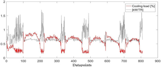
Figure 6.
Load profile and efficiency for a centrifugal chiller for a week of September 2018.
Similarly, Tci is a crucial variable linked to a cooling tower. Further work is dedicated to analyzing the effect of the condenser water inlet temperature through a cooling tower model integrated to Equation (22). Some research could be done in the direction of estimate the consumption of a whole chiller plant.
It is crucial because, from Figure 5, it is evident that the chiller operates much time at partial load and is necessary to analyze equipment irreversibilities in order to improve the performance of this centrifugal chiller. To evaluate COP and consumption, scatter charts have been plotted (see Figure 7, Figure 8).
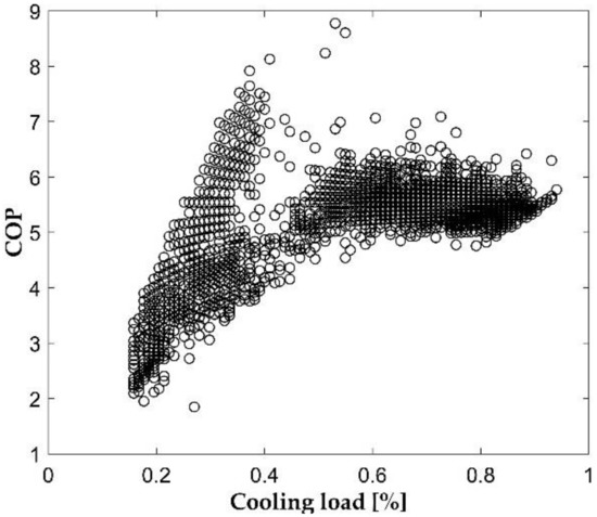
Figure 7.
Cooling load (%)–coefficient of performance (COP) plot for September 2018 data.
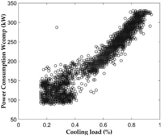
Figure 8.
Cooling load (%)–Wcomp plot for September data.
From plots 7 and 8, it is observed that according to theory [7,8] at low cooling rates, it seems to appear linear behavior between cooling load and COP dominated by losses as fluid friction and throttling. At high cooling rates, the curve is dominated by losses from heat transfer. Input power is proportional to the cooling load above 50%, but it is not clear at low cooling rates. Chiller performance is related to the three physical parameters. Those can be estimated by analysis and regression. Table 4 shows the values for every model regression applied to data and sub-data filtered with their corresponding ER%. For all sub-data, there is a good accuracy of the parameter R with ER% below 10%. Qleak,eq and Sgen show poor accuracy; this is because of the strong dependency of the cooling rate that makes it hard to assume a constant term. Centrifugal chiller control by variable speed driver (VSD) and prerrotation vanes (PRV) influence Sgen generating significant friction at low cooling load. The better accuracy has been achieved close to Tcho set point (6.7 °C) when it is expected a more stable operation. See Figure 9 to observe the behavior of the physical parameters for the sub-data of September. Qleak,eq and Sgen are highly dynamic. Values listed in Table 4 are averaged values; in the same way, the regressor parameters are assumed as constant, but they are not. However, the heat exchanger’s thermal resistance is very stable, with few critical peaks which correspond to cooling load peaks.
Table 4.
Physical parameters estimated by regression and an algorithm for the September sub-data.
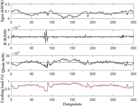
Figure 9.
Physical parameters profiles and Cooling load percent to compare behavior for September sub-data.
Centrifugal chillers have been used to provide large cooling in buildings, and their efficiency is high, as observed in the present work. Even though they seem to have stable behavior, they are exposed to dynamical changes in loads and temperatures so that any steady-state model will be inaccurate. For the 550 TR chiller plant facility, not all the data was available due to limitations in the control system, and for that reason, many assumptions were made to develop a simple thermodynamic model. From Figure 6, Figure 7 and Figure 8, it is clearly noticed that there is a segmented range of operation with different load regimes. Because of that, different behavior could be expected for each segment. However, it is possible to find a model with enough robustness for both: low and partial load.
The fundamental model GNU depends on assumptions made to its development and final terms. Original authors [8] validate the approximations for A, B, C, and based on experimental measures for reciprocating chillers. The rearranged model proposed in this paper applied to centrifugal chillers should be validated, too, for the same approximations. Table 5 shows the values of the coefficients denoting the suitability of the model.
Table 5.
Approximation of coefficients used to develop the model GNU rearranged.
3.1. Validation with Training Data
Training data extracted from September data has been used to fit three models in order to compare their internal prediction power: GNU, GNU rearranged, and Braun. Metrics R2, R2adj, MRE, and CV are shown in Figure 10 and Figure 11. Braun model has a CV of less than 5% except for the larger data. MRE is less than 10% for all the sub-data, which demonstrates good accuracy for Braun empirical model. However, parameters of this model do not have physical significance for thermodynamic performance purposes; they only would be useful for external prediction or fault detection and diagnosis. In the case of semiempirical models, MRE is less than 10% for both GNU and GNU rearranged. Also, both of them achieved CV less than 5% for the sub-data close to the setpoint, but GNU does not have a good square correlation R2 (41%), while GNU rearranged has an excellent R2 (97%). In all cases, the Braun model has better accuracy than the rearranged model. This result fits with the good performance of the model in the literature. However, the Braun model is empirical, and its coefficients have no practical meaning, which makes the Braun model an excellent predictive tool but less useful to evaluate performance through physical parameters. (see Figure 11).
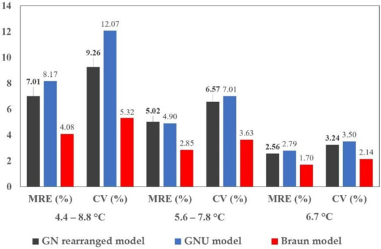
Figure 10.
Comparison of mean relative error (MRE) and the coefficient of variation (CV) of three models for various sub-data.
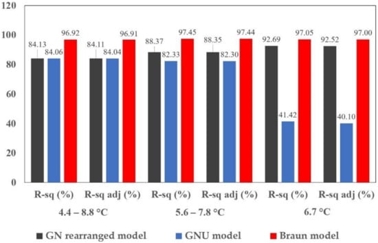
Figure 11.
Comparison of R2 and R2 adjusted of three models for various sub-data.
From Figure 9, Figure 10 and Figure 11 is possible to analyze the relationship between the physical parameters and accuracy of the GN models. As the subdata is close to the set point the more the model is accurate. Values close to setpoint is reflected in a stabilized behavior of the parameters Sgen, Qleak,eq and R. another consequence is the assumption of constancy of those parameters linked to the steady-state framework of the model.
Other works over centrifugal chillers [10] show better metrics for the GNU model (CV below 5%) applied to the same capacities (550 TR). The water flow rates are also constant, but they are not explicit about the type of control used for partial loads. GNU fundamental model was not designed over centrifugal chillers with variable speed drives, and inlet guide vanes control used at the same time, and it is not accurate enough when dealing with dynamic changes caused by these types of control. Variation in pressure and flow rate must be reflected in COP, which is an instantaneous parameter. By modifying the GNU model, consumption and cooling load can be obtained as an average of cumulative values, which are measured in a period and are not instantaneous.
In addition, changing variables help to stabilize unbiased data. An example of this can be seen in Figure 12, where the independence of residuals for both models is depicted. Based on metrics and predicted values (Figure 13), GNU rearranged model achieves good internal accuracy to estimate energy consumption and to analyze performance.
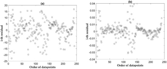
Figure 12.
(a) Independence of i-th residuals for Gordon–Ng (GNU) rearranged model. (b) Independence of i-th residuals for the GNU model.
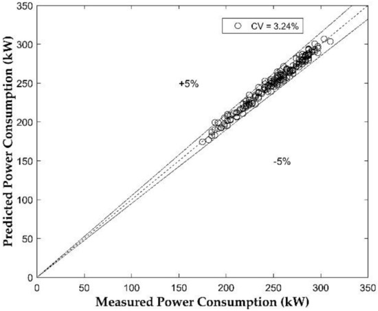
Figure 13.
Results of the accuracy of the GNU modified model.
The three physical parameters: internal entropy generation, rate of heat losses or gain from the chiller, and total heat exchanger thermal resistance, were compared with the values obtained by an algorithm in order to examine the influence of including the intercept term. Results are listed in Table 6 next to ER%. It should be noted that the GNU rearranged model as well as GNU model do not estimate the physical parameters when the interception term is included. From Table 6, it is evident that ER% is larger than 100%. Furthermore, there is a negative value for the entropy generated by the GNU model. Summarizing, models with interception terms are not useful to estimate parameters, nevertheless, they can be used for prediction.
Table 6.
Physical parameters estimated by regression with the intercept term and an algorithm for the September sub-data.
3.2. Validation with Testing Data
Testing data for July 2018 was obtained from the BAS system, it is not used to fit models, but it is collected from the same equipment. For that reason, it is used to validate the prediction capacity outside the training data. Every sub-data was averaged and tested. The results are listed in Table 7.
Table 7.
Comparison of MRE and CV of three models for various sub-data.
It would be expected to achieve a better external prediction accuracy where the internal prediction was the best. Results show that a GNU customized model estimates consumption with better accuracy than other models for testing data, being CV% improved for extensive averaged testing data. MRE is less than 10% for both GNU models and below 5% for GNU modified. Braun model does not have good accuracy for testing data. Additional research must be done in this area. Figure 14 plots the power prediction of each model.
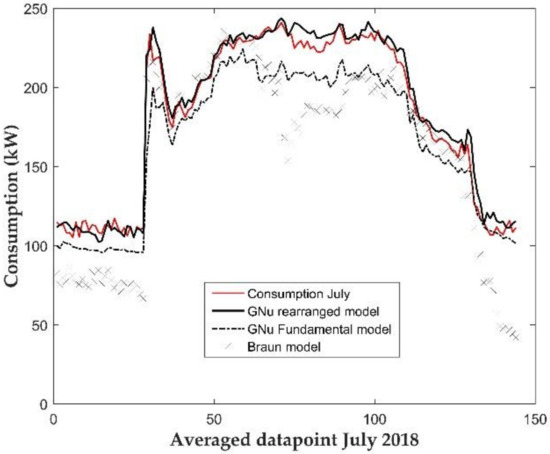
Figure 14.
Consumption profile plot showing external prediction for each model.
The two GNU models show similar behavior at low cooling rates (reflected as power consumption) except the Braun model that overestimates values. Dynamic changes are not well captured in the whole operation. GNU rearranged overestimates values of consumption at partial and high loads, especially peak values.
3.3. Toward Validation with Any External Data
Empirical based models are applicable only for the same range of data from which they were fitted. However, it is valuable to validate the proposed model for the same centrifugal chiller under another set of conditions. Future work is in the direction of getting a new data set from another month of the year 2018. There is an interest in investigating the behavior of the model after and before maintenance routines. As has been set the scope of better accuracy, the proposed model should include the parameters regressed listed in the first row of Table 6. The proceedings are as follows:
- Definition of the operational range of the new data set. Recognition of atypical values and temperature setpoints.
- Introduction of parameters of the consumption model, according to the required accuracy.
- Data filtering. Then, it can be created each sub-data listed in Table 7.
- Validation for each sub-data. Estimation of accuracy through appropriate metrics.
- Comparison of results and analysis.
If the power prediction is not successful, it should be explored possible factors that could impact some of the parameters, as maintenance routines or operational changes (setpoints, building loads).
4. Conclusions
In this paper, a thermodynamic modeling analysis was proposed to analyze, predict, and optimize the performance of a centrifugal chiller. According to a simple thermodynamic analysis (several assumptions were made), a steady-state model was built based on easy measured variables and three physical parameters which can be obtained by regression. The three parameters were also estimated through an algorithm built from a thermodynamic analysis of the steady-state cycle. After comparation between the fundamental GNU and the proposed model was found that the proposed model showed less ER% for the thermal resistance of heat exchangers (less than 5%) and ER% below 20% for entropy generation and leak energy, for a sub-data close to the setpoint value, 6.7%. Two sets of data were used, a training data corresponding to September and testing data (split in two) from July in order to validate internal and external prediction, respectively. It was also proved that the appropriate inclusion of an intercept term is valuable if the aim of the model is only for prediction purposes. The validation of assumptions made by GNU model along centrifugal chillers, was made. however, further experimental work should be made and contrasted with the results obtained here.
Analysis indicates that (for internal data), the accuracy of the proposed model is better than the fundamental GNU and close to the Braun model. With R2 and CV of 92%, 40%, 97% and 3.24%, 3.50%, 2.14%, respectively. The model achieved better accuracy as the sub-data is filtered around the setpoint value, where the operation is stable. External validation through an average testing data denoted good accuracy, with CV% less than 5% comparing to GNU and Braun models, but it tends to overestimate high cooling loads. It is essential to keep in mind that models are developed under steady-state and ideal conditions, without considering control routines/devices. Further work will be done in this direction. Also, it is necessary to develop dynamic modeling for vapor compression cycles considering the simultaneous effects of inlet guide vanes and the variable speed driver.
Author Contributions
Conceptualization, B.F. and A.B.; methodology, B.F.; validation, B.F.; formal analysis B.F. and A.B.; investigation, B.F.; resources, A.B.; writing—original draft preparation, B.F.; writing—review and editing, B.F., A.B. and P.C.; visualization, B.F.; supervision, A.B. and P.C.; project administration, A.B. and P.C.; funding acquisition, B.F., A.B. and P.C. All authors have read and agree to the published version of the manuscript.
Funding
This research was funded by Colciencias through Convocatoria Doctorados Nacionales 727 of Fondo Nacional de Financiamiento para la Ciencia, la Tecnología e Innovación FCTeI, by Sistema General de Regalías SGR and Universidad del Norte.
Acknowledgments
The authors would like to thank Universidad del Norte and Colciencias through Convocatoria Doctorados Nacionales 727 of Fondo Nacional de Financiamiento para la Ciencia, la Tecnología e Innovación FCTeI, by Sistema General de Regalías SGR for supporting this research.
Conflicts of Interest
The authors declare no conflict of interest. The funders had no role in the design of the study, in the collection, analyses, or interpretation of the data.
Abbreviations and Nomenclature
| AHRI | Air Conditioning, Heating, and Refrigerant Institute |
| BAS | Building Automation system |
| BQ | Bi-quadratic regression model |
| COP | Coefficient of performance |
| CV | Coefficient of variation |
| ER | Relative Error |
| FDD | Fault detection and diagnosis |
| GNU | Fundamental Gordon–Ng model |
| GNS | Universal Gordon-Ng model |
| PRV | Inlet guide vane control (Prerrotation vanes) |
| MP | Polinomial regression model |
| MRE | Mean Relative error |
| TR | Tons of refrigeration |
| VSD | Variable speed driver |
| c | heat capacity |
| T | temperature |
| Sgen | generated entropy |
| Q | heat transfer |
| Wcomp | power consumption |
| C | thermal capacitance |
| mass flow | |
| r | corrected thermal capacitance |
| R | heat exchanger thermal resistance |
| h | enthalpy |
| ε | heat exchanger effectiveness |
| Subscripts | |
| c | condenser |
| cw | condenser, cooling water side |
| ev | evaporator, refrigerant side |
| ch | evaporator, cooling water side |
| i | inlet |
| o | oulet |
| ci | condenser cooling water inlet |
| co | condenser cooling water outlet |
| ref | refrigerant |
| sat | saturation condition |
| LT | total leak |
| lev | evaporator leak |
| lc | condenser leak |
| lcomp | compressor leak |
| leak,eq | equivalent leak |
| comp | compressor |
| dis | discharge |
| des | design |
| sh | superheating |
References
- Kim, W.; Katipamula, S. A review of fault detection and diagnostics methods for building systems. Sci. Technol. Built Environ. 2018, 24, 3–21. [Google Scholar] [CrossRef]
- Romero, J.A.; Navarro-Esbrí, J.; Belman-Flores, J.M. A simplified black-box model oriented to chilled water temperature control in a variable speed vapour compression system. Appl. Therm. Eng. 2011, 31, 329–335. [Google Scholar] [CrossRef]
- Lee, T.-S.; Liao, K.-Y.; Lu, W.-C. Evaluation of the suitability of empirically-based models for predicting energy performance of centrifugal water chillers with variable chilled water flow. Appl. Energy 2012, 93, 583–595. [Google Scholar] [CrossRef]
- Jiang, W. Reevaluation of the Gordon-Ng performance models for water-cooled chillers. ASHRAE Trans. 2003, 109 (Pt 2), 272–287. [Google Scholar]
- Reddy, T.A.; Niebur, D.; Andersen, K.K.; Pericolo, P.P.; Cabrera, G. Evaluation of the suitability of different chiller performance models for on-line training applied to automated fault detection and diagnosis (RP-1139). HVAC R Res. 2003, 9, 385–414. [Google Scholar] [CrossRef]
- Braun, J.E. Methodologies for the Design and Control of Chilled Water Systems. Ph.D. Thesis, University of Wisconsin, Madison, WI, USA, 1988. [Google Scholar]
- Gordon, J.; Ng, K.C.; Chua, H.T. Centrifugal chillers: Thermodynamic modelling and a diagnostic case study. Int. J. Refrig. 1995, 18, 253–257. [Google Scholar] [CrossRef]
- Ng, K.C.; Chua, H.T.; Ong, W.; Lee, S.S.; Gordon, J.M. Diagnostics and optimization of reciprocating chillers: Theory and experiment. Appl. Therm. Eng. 1997, 17, 263–276. [Google Scholar] [CrossRef]
- Gordon, M.J.; Ng, K.C. Cool Thermodynamics: The Engineering and Physics of Predictive, Diagnostic and Optimization Methods for Cooling Systems; Cambridge International Science Publishing: Cambridge, UK, 2000. [Google Scholar]
- Lee, T.S.; Lu, W.C. An evaluation of empirically-based models for predicting energy performance of vapor-compression water chillers. Appl. Energy 2010, 87, 3486–3493. [Google Scholar] [CrossRef]
- Browne, M.W.; Bansal, P.K. Different modelling strategies for in situ liquid chillers. Proc. Inst. Mech. Eng. Part A J. Power Energy 2001, 215, 357–374. [Google Scholar] [CrossRef]
- Swider, D.J. A comparison of empirically based steady-state models for vapor-compression liquid chillers. Appl. Therm. Eng. 2003, 23, 539–556. [Google Scholar] [CrossRef]
- Wang, H. Empirical model for evaluating power consumption of centrifugal chillers. Energy Build. 2017, 140, 359–370. [Google Scholar] [CrossRef]
- Wang, H. A steady-state empirical model for evaluating energy efficient performance of centrifugal water chillers. Energy Build. 2017, 154, 415–429. [Google Scholar] [CrossRef]
- Reddy, T.A.; Andersen, K.K. An evaluation of classical steady-state off-line linear parameter estimation methods applied to chiller performance data. HVAC R Res. 2002, 8, 101–124. [Google Scholar] [CrossRef]
- Jia, Y.; Reddy, T.A. Characteristic Physical Parameter Approach to Modeling Chillers Suitable for Fault Detection, Diagnosis, and Evaluation. J. Sol. Energy Eng. 2003, 125, 258–265. [Google Scholar] [CrossRef]
- Saththasivam, J.; Tang, G.; Ng, K.C. Evaluation of the simple thermodynamic model (gordon and ng universal chiller model) as a fault detection and diagnosis tool for on-site centrifugal chillers. Int. J. Air Cond. Refrig. 2010, 18, 55–60. [Google Scholar] [CrossRef]
- Saththasivam, J.; Ng, K.C. Predictive and diagnostic methods for centrifugal chillers. ASHRAE Trans. 2008, 114 (Pt 1), 282–287. [Google Scholar]
- Yu, F.W.; Ho, W.T. Multivariate diagnosis analysis for chiller system for improving energy performance. J. Build. Eng. 2018, 20, 317–326. [Google Scholar] [CrossRef]
- Wang, Y.; Jin, X.; Du, Z.; Zhu, X. Evaluation of operation performance of a multi-chiller system using a data-based chiller model. Energy Build. 2018, 172, 1–9. [Google Scholar] [CrossRef]
- Beaulieu St-Laurent, P.; Gosselin, L.; Duchesne, C. Analysis and prediction of chilled water plant performance based on multivariate statistical methods and large historical data. Int. J. Refrig. 2018, 90, 132–144. [Google Scholar] [CrossRef]
- Yu, F.W.; Ho, W.T. Assessing operating statuses for chiller system with Cox regression. Int. J. Refrig. 2019, 98, 182–193. [Google Scholar] [CrossRef]
- Li, M.; Ju, Y. The analysis of the operating performance of a chiller system based on hierarchal cluster method. Energy Build. 2017, 138, 695–703. [Google Scholar] [CrossRef]
- Halon, T.; Pelinska-Olko, E.; Szyc, M.; Zajaczkowski, B. Predicting performance of a district heat powered adsorption chiller by means of an artificial neural network. Energies 2019, 12, 3328. [Google Scholar] [CrossRef]
- Acerbi, F.; De Nicolao, G. Identification of the gordon-ng chiller model: Linear or nonlinear least squares? In Proceedings of the 2018 IEEE 23rd International Conference on Emerging Technologies and Factory Automation (ETFA), Turin, Italy, 4–7 September 2018; pp. 1314–1321. [Google Scholar]
- Acerbi, F.; De Nicolao, G.; Obiltschnig, J.; Richter, P.; De Luca, C. Accuracy and robustness against covariate shift of water chiller models. In Proceedings of the 2018 IEEE 14th International Conference on Automation Science and Engineering (CASE), Munich, Germany, 20–24 August 2018; pp. 809–816. [Google Scholar]
- AHRI Standard 550/590. Performance Rating of Water-Chilling and Heat Pump Water-Hetaing Packages Using the Vapor Compression Cycle; Air Conditioning, Heating, and Refrigeration Institute: Arlington, VA, USA, 2018.
- Beyene, A.; Guven, H.; Jawdat, Z.; Lowrey, P. Conventional chiller performances simulation and field data. Int. J. Energy Res. 1994, 18, 391–399. [Google Scholar] [CrossRef]


© 2020 by the authors. Licensee MDPI, Basel, Switzerland. This article is an open access article distributed under the terms and conditions of the Creative Commons Attribution (CC BY) license (http://creativecommons.org/licenses/by/4.0/).