Abstract
Dynamic Mode Decomposition (DMD) techniques have risen as prominent feature identification methods in the field of fluid dynamics. Any of the multiple variables of the DMD method allows to identify meaningful features from either experimental or numerical flow data on a data-driven manner. Performing a DMD analysis requires handling matrices , where and N are indicative of the spatial and temporal resolutions. The DMD analysis of a complex flow field requires long temporal sequences of well resolved data, and thus the memory footprint may become prohibitively large. In this contribution, the effect that principled spatial agglomeration (i.e., reduction in via clustering) has on the results derived from the DMD analysis is investigated. We compare twelve different clustering algorithms on three testcases, encompassing different flow regimes: a synthetic flow field, a flow around a cylinder cross section, and a turbulent channel flow. The performance of the clustering techniques is thoroughly assessed concerning both the accuracy of the results retrieved and the computational performance. From this assessment, we identify DBSCAN/HDBSCAN as the methods to be used if only relatively high agglomeration levels are affordable. On the contrary, Mini-batch K-means arises as the method of choice whenever high agglomeration is possible.
1. Introduction
The characterization of complex flow phenomena is typically attained by resorting to experimental (Laser Doppler Anemometry, Particle Image Velocimetry, …) and/or numerical (Computational Fluid Dynamics simulations) tools. Feature extraction algorithms can be leveraged for the classification of the –typically, massive amounts of– data involved. Perhaps the most common strategies are the Proper Orthogonal Decomposition (POD) and the Dynamic Mode Decomposition (DMD) techniques.
Proper Orthogonal Decomposition techniques, ([1,2,3,4])—also known as Principal Component Analysis or Karhunen-Loève decomposition– operate on sequences of snapshots, that is, either experimental measurements or numerical solutions acquired at successive time instants. An optimal representation of the sequence is provided by the POD method, as features identified by POD are orthogonal to each other [4]. Recently, techniques to perform Spectral POD have been described in References [5,6,7].
Other alternative feature identification strategies exist, for example, the Empirical Mode Decomposition (EMD), which is closely related to the Huang-Hilbert transform [8]. The EMD has been recently leveraged to discriminate large from small turbulent structures and characterize phenomena like modulation and footprinting in channel flows [9,10].
Dynamic mode decomposition techniques, which emerged about ten years ago with the seminal contributions of Schmid [11] and Rowley and collaborators [12], have arisen as prominent feature identification methods in the field of fluid dynamics. Any of the multiple variants of the DMD method [11,12,13,14,15] allows to identify meaningful flow features from either experimental [16,17,18] or numerical flow data [19,20,21,22] in a purely data-driven (equation free) manner [23].
The analysis of ever increasingly complex flow fields leads to more and more stringent computational constraints. In order to contextualize the discussion—which we will extend in Section 2—let us advance that performing a classical DMD analysis as those presented in Reference [11] requires handling matrices , where and N are indicative of the spatial and temporal resolutions, respectively. Since the analysis of a complex flow field requires, in general, long temporal sequences of well resolved data, the memory footprint to accomplish a DMD analysis can easily become prohibitively large.
In order to face this situation, several strategies have been considered so far. One of those strategies resorts to parallelism: Sayadi and Schmid proposed a memory distributed parallel DMD algorithm in reference [24], which they used to analyze laminar-turbulent transition in a flat plate. Alternatively, Grenga et al. [21] described another parallel implementation of DMD used in the analysis of a turbulent combustion problem.
Another approach leading to computationally tractable problems attempts to reduce—in a principled manner—the memory footprint of the input data sequence. This reduction can be accomplished following a number of techniques. Randomized DMD (rDMD) algorithms (see e.g., References [25,26]) exploit principles of stochastic nature [27] to compute a near-optimal low-rank DMD decomposition of the input data sequence. DMD formulations benefiting from compressed sensing principles have also been proposed, see Reference [28]; Reference [29] describes a derived technique that successfully accomplishes background modeling for video applications.
An alternative yet similar approach is that of Guéniat et al.; they proposed in Reference [30] a variant of DMD—the Non-Uniform DMD or NU-DMD algorithm—that attempts to represent the input data sequence, in certain optimal sense, at a reduced cost. The NU-DMD algorithm proposes two possible avenues to reduce the computing cost: the first considers the possibility to represent the temporal dynamics of the data sequence with a reduced number of snapshots (temporal compression), that is, with a shorter (and perhaps non-uniformly sampled in time) data sequence . The second opportunity comes from the possibility of identifying a small subset of degrees of freedom (DoFs), each of them representing –in an optimal sense– the dynamics of many other DoFs. In other words, those many DoFs are agglomerated into a single DoF whose behavior is descriptive of the behavior of the whole cluster. In Reference [30], the spatial reduction was attained via the application of the K-means algorithm.
In this contribution we explore a possible avenue to alleviate the computational cost associated to the data-driven DMD analysis of complex flow fields: following Reference [30], we investigate how the principled reduction of the data matrix using different unsupervised learning algorithms affects the quality of the results that DMD can obtain. The mathematical framework set in Reference [28] will be also useful for this approach.
As we shall justify in Section 3, reductions in the leading (spatial) dimension of the data matrices are potentially more beneficial than reductions in the second (temporal) dimension N, see Figure 2 and the associated discussion. Accordingly, in this contribution we assess thoroughly the effect that twelve different spatial agglomeration techniques have on the flow features identified by classical DMD. The performance evaluation of the Spatially Agglomerated DMD goes beyond the measurement of the possible reductions in the computational burden (memory footprint and/or computing time): the physical relevance of the features identified in the analysis is also taken into consideration.
The aforementioned evaluation will be conducted on three different test cases, encompassing a wide range of flow phenomena. The first testcase considered is a toy model, a synthetic flow field studied already in References [16,30]. The second testcase considered is the flow around the mid section of infinitely long cylinder [20], whereas the third testcase is the turbulent channel flow at [31,32].
The rest of this paper is organized as follows: Section 2 introduces both the specific DMD algorithm and the dozen of spatial agglomeration techniques studied in this work. Next, Section 3 introduces the testcases considered, describes the results obtained and assesses the performance of the different clustering methods studied. Finally, Section 4 presents the conclusions attained and provides several recommendations.
2. Methodology
In this section, we present the methodology employed throughout this work. Section 2.1 introduces the specific implementation of the DMD algorithm considered Next, the different clustering algorithms considered are briefly presented in Section 2.2. Finally, Section 2.3 addresses the reconstruction of global features from the clustered data.
2.1. Dynamic Mode Decomposition
Consider a sequence of instantaneous flow fields, or data snapshots , indexed from 1 to N. These snapshots are often solutions of a (possibly non-linear) dynamic system given by:
Alternatively, they could be the result of a flow measurement process, for example, Particle Image Velocimetry images. Irrespective of their origin, recasting the snapshots as vectors (and , with the number of spatial locations considered and the number of magnitudes, e.g. pressure, temperature, …, recorded) and stacking them we can assemble a data matrix:
Two successive snapshots are separated by the (non-necessarily uniform) time interval such that for all . In the case of linear stability analysis and within the exponential growth region, it is possible to define a linear operator (i.e., a numerical approximation of the linearized Navier–Stokes operator) such that . For non-linear systems, approximates the Koopman operator [33]. Equation (2) can then be rewritten as a Krylov sequence (see Reference [34]):
Several well established implementations of the DMD algorithm exist; here we follow mainly [11]. The DMD based analysis of data sequence in Equation (2) (which we consider uniformly sampled in time) begins with the economy sized Singular Value Decomposition (SVD) of the subsequence . Superscript H denotes conjugate transposition, matrix is a diagonal matrix with entries the singular values, and the left singular vectors—the columns of —can be related to the POD modes of the input data sequence [35]. Inserting the SVD of the snapshot matrix into Equation (5) yields . Some algebra leads to the reduced matrix , the projection of the matrix onto the space contained in .
Both the reduced DMD modes and the associated eigenvalues/Ritz values are obtained by solving the eigenvalue problem . Approximated eigenmodes of the matrix are recovered through projection onto the original space, that is, . Provided , the growth rates and frequencies in the complex half-plane are given as , which we obtain from relation .
The j-th snapshot can be expanded in the DMD basis as:
The matrix counterpart of the previous expression is:
where the columns in matrix are the dynamic modes , is the diagonal matrix with the amplitudes and is a Vandermonde matrix built using the Ritz values. Note that the amplitudes are identified through a minimization problem in the unitarily invariant Frobenius norm (more details in Reference [36]):
Since matrix is unitary, it does not affect the norm in Equation (8), and the optimization problem actually solved is:
with the columns in matrix the eigenvectors of matrix .
Finally, note the upper limit in the expansion given by Equation (6): if a smaller number is considered -namely, if this expansion is truncated- a reduced order model for the database is obtained.
2.2. Spatial Agglomeration Strategies
The DMD technique described in Reference [30] employs the K-means algorithm to agglomerate the spatial degrees of freedom. The goal was to find, in a principled manner, space-decimated subsets of the input data-sequence that simultaneously convey the dominant temporal information.
In this contribution, we investigate the effect that different spatial agglomeration techniques have on the features identified by the DMD algorithm described in Section 2.1. Both computational savings and relevance of the physical phenomena captured by DMD are considered in the study. In total, a dozen of different spatial agglomeration techniques are compared. Among them, we have studied a number of variants of the K-means algorithm.
Before proceeding with the introduction and description of the spatial agglomeration techniques, we advance a number of preliminary thoughts.
First, recall that Guéniat et al. [30] found that the first (estimated) statistical moments serve as a convenient means to drive the spatial clustering process. Indeed, they argue that those spatial degrees of freedom whose first statistical moments are relatively close to each other are good candidates for being agglomerated into a single cluster. We follow their lead, and throughout our investigation, we resort to the first estimated central moments to guide the agglomeration of spatial DoFs.
Second, note that the outcome of all the agglomeration techniques considered is a set of clusters. However, not every algorithm provides explicitly a specific degree of freedom (i.e., a centroid) representative of the members of the cluster. In those cases, a centroid was randomly selected from the spatial location belonging to the cluster. Also, not all the algorithms considered accept as an input parameter: In those cases, the controlling parameters were adjusted to obtain a number as close as possible to the desired one.
Finally, the research has been conducted using the python language (version ); most of the spatial agglomeration algorithms are provided either from SciPy [37] or Scikit-learn [38] libraries. Whenever a different python package is used, it is also indicated.
In what follows we enumerate and provide a brief description of the agglomeration techniques considered; Table 1 offers a summary of the techniques employed.

Table 1.
Summary of the spatial algorithms considered.
- Classical K-means, from scikit-learn: It is one of the simplest and most popular unsupervised machine learning algorithms. In a few words, the algorithm identifies first centroids; every data point is associated to the nearest cluster. Let be the number of centroids and suppose the algorithm needs I iterations to converge (we should speak then of -means algorithm, but in order to ease the discussion, we have decided to maintain the K-means terminology). The space complexity of K-means clustering algorithm is . Based on the number of distance calculations, the time complexity of K-means is [39].
- Mini-batch K-means, from scikit-learn: A variant of the K-means algorithm which uses mini-batches (subsets of the input points, randomly sampled in each iteration) to reduce the computation time, while still attempting to optimize the same objective function as K-means does, see Reference [40].
- Classical K-means, from SciPy: Same as method 1, but provided by Reference [37];
- K-means++, from SciPy: This variant of the K-means, through a randomized seeding of the initial K centers, typically achieves a solution faster than the standard algorithm [41].
- DBSCAN, from scikit-learn: The DBSCAN (Density-based spatial clustering of applications with noise [42]) interpretes clusters as high density regions separated by areas of low density. The cluster density is controlled by two parameters: the maximum distance between points in the same cluster the minimum number of points needed to form a cluster . The DBSCAN runtime complexity is , where indicates the cost of computing the distance, whereas the spatial complexity is roughly [43]. In this work, the maximum distance allowed is set to and the minimum number points per cluster is .
- HDBSCAN, from HDBSCAN: HDBSCAN is a hierarchical extension of DBSCAN, which uses unsupervised learning to find clusters in the dataset. The runtime complexity is [44].
- C-Means, from SciPy/skfuzzy: C-Means (also known as Fuzzy C-means, FCM) [45]. resembles K-means algorithms, though it employs a fuzzifier and handles membership values: differently from K-means, a degree of freedom is allowed to belong to several clusters.
- Gaussian Mixture, from scikit-learn: This method ([46,47]) enables one to learn Gaussian Mixture Models, sample them, and estimate them from data. It implements the expectation-maximization algorithm for fitting models, draw confidence ellipsoids for multivariate models, and compute the Bayesian Information Criterion to assess the number of clusters in the data. The temporal complexity is : is the number of Gaussian components, which needs to be chosen carefully to control the computational cost [46].
- Mean Shift, from scikit-learn: Mean shift is a non-parametric feature-space analysis technique for locating the maxima of a density function, a so-called mode-seeking algorithm. The density function (typically a Gaussian kernel) determines the weight of nearby points for re-estimation of the mean, and replace the cores points with weight mean value by iteration until converged. Application domains include cluster analysis in computer vision and image processing [48]. The classic mean shift algorithm has spatial and temporal complexities of, respectively, and , with I the number of iterations.
- Affinity Propagation, from scikit-learn: In statistics and data mining, affinity propagation (AP) is a clustering algorithm based on the concept of “message passing” between data points. It does not require the number of clusters to be determined or estimated before running the algorithm but it still finds members of the input set that are representative of clusters [49]. The runtime complexity is .
- Agglomerative Clustering, from scikit-learn: It is perhaps the most common type of hierarchical clustering used to group objects in clusters based on their similarity. It resembles HDBSCAN, though it is more effective with multi-scale datasets. However, the standard algorithm for hierarchical agglomerative clustering has a time complexity of and has a memory footprint of . This makes the algorithm potentially unsuited for moderately large datasets.
- BIRCH, from scikit-learn: BIRCH (balanced iterative reducing and clustering using hierarchies) is an unsupervised data mining algorithm used to perform hierarchical clustering over particularly large data-sets [50]. In some cases, BIRCH requires a single pass on the database and can achieve a computational complexity of .
2.3. Reconstruction of DMD with Agglomeration
As we have just seen, the clustering techniques in Section 2.2 can serve as enablers for the potentially costly DMD analysis of the input data matrix . Direct application of those techniques will provide approximated Ritz values, ’s, indicative of the frequency and temporal growth (or attenuation) of the features identified. However, the spatial support of the associated dynamic mode is restricted to the agglomerated space. In other words, , with . The legitimate question on how to relate and arises.
For this task, it is useful to refer to compressed sensing theory, and specifically to the measurement matrix discussed in cDMD [28]. The following relation holds:
Recasting the individual modes and as columns of matrices and , leads to the compact matrix form:
Recall that the clustering is driven [30] by the estimated statisical moments computed at every computational grid point. Those moments are arranged in matrix is then fed to any of the clustering algorithms considered. The outcome of the agglomeration process allows to build the measurement matrix , as a subset of rows taken from the identity matrix . In this sense, has a purely geometric interpretation.
The reconstructed modes are obtained, following [28], using the following relation:
In the equation above, matrices and are obtained from the SVD decomposition of the reduced dataset , whereas matrix is obtained from the eigenvalue decomposition of matrix . This relation (12) will be specially useful in Section 3.2 and Section 3.3.
3. Results
As we discussed in Section 2, the goal of this work is to perform a thorough assessment of the performance of DMD when applied to databases that have been reduced using different spatial agglomeration techniques. In order to obtain conclusions that are as informative as possible, we have considered three testcases, encompassing different flow regimes.
The first testcase pertains to a one-dimensional field with spatio-temporal dependence. Despite its simplicity, this flow is very useful nevertheless, as it provides a good example of why reducing the input data matrix along its leading dimension is potentially more profitable than reducing it along its second dimension. Additionally, this testcase will allow us to establish a metrics allowing a fair comparison of the different spatial agglomeration techniques considered.
The second testcase is the the flow field around the mid-section of a very long cylinder. This flow is mainly laminar, but the fact that makes this problem rich enough to study with DMD.
Finally, the turbulent channel flow field along two indefinitely long plates is considered. The multiscale nature of the problem makes it a challenging test for the DMD analysis of the spatially agglomerated database.
All the computations described have been performed on a computer equipped with an 4-core Intel Core i5-3570K CPU at 3.40 GHz, a cache memory of 6144 kB and 8.0 GB of RAM.
3.1. A Toy Model: The Synthetic Field
As the first testcase, we consider a synthetic field given by Equation (13).
This toy model is one-dimensional, presents both spatial and temporal variations and has been already investigated in References [16,30]. Following Reference [30], we consider angular pulsation (and hence, frequency ) and temporal growth rate . The initial amplitude , the wavenumber and the spatial growth rate are all set to 1. The spatio-temporal domain is discretized with equispaced points in and equiseparated temporal samples in the time interval . Note that having is quite uncommon. In typical flow data bases (specially those obtained from CFD calculations, , or even ); we consider this analysis for consistence with previous work [30]. The robustness of the decomposition methods is tested by introducing white multiplicative noise , in an attempt to mimic the deviation in the real data from an experiment. The Noise to Signal Ratio () is set to . Figure 1 shows the noise-corrupted database employed in our analysis, together with the clean field for comparison.
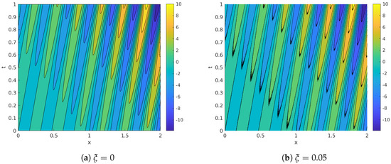
Figure 1.
Synthetic system: clean (a) and noisy (b) fields.
3.1.1. Motivational Experiment: Spatial Agglomeration and Temporal Compression
Before proceeding with the comparison of the different spatial agglomeration techniques we describe a first, motivational experiment. The experiment consists in applying DMD to the noisy synthetic database and progressively reduced versions of it. Two alternative reductions are considered: on the one hand, reductions along the spatial dimension (or spatial agglomeration) are performed using the Scikit-learn implementation of the classical K-means algorithm. On the other hand, reductions along the temporal dimension (or temporal compression) is accomplished by simply considering decimated subsequences taken from the discretization of the temporal variable. Increasing levels of spatial agglomeration and temporal compression were considered: 30 points logarithmically distributed in the range (no agglomeration/compression) to , which for the temporal compression case corresponds approximately with the Nyquist frequency.
Figure 2 summarizes the results of the experiment. Focusing on the most relevant feature identified by DMD, Figure 2a shows the map of the normalized frequency error, , whereas Figure 2b shows the normalized error commited in the temporal growth rate, .
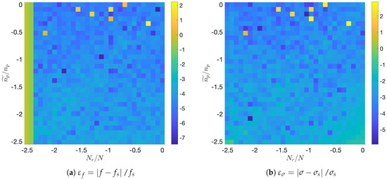
Figure 2.
Synthetic system: Relative errors in frequency (a) and growth rate (b) with uniform temporal compression and spatial reduction using K-means algorithm, in a scale.
Inspection of Figure 2a shows how normalized errors in frequency are mostly around . Several points with higher error appear isolatedly at low levels of agglomeration (topmost part of the graph). The Nyquist cut-off limit is also clearly visible, for every agglomeration level, in the leftmost part of the graph as a marked increased in error.
The analysis of Figure 2b shows that error levels for the temporal growth are also around . Several isolated points with high error appear as well at low agglomeration levels.
In this work we will favor spatial agglomeration over temporal reduction for several reasons: first, because in in most realistic databases ; second, because spatial agglomeration is not limited from below by the Niquist constraint; and finally because most DMD variants described in the bibliography require temporally equiseparated snapshots. We proceed now with the comparison of the dozen spatial agglomeration techniques presented in Section 2.2.
3.1.2. DMD Analysis of Spatially Agglomerated Synthetic System: Assessment of Clustering Algorithms
Figure 3 shows how closely the frequency and growth rate are captured by the DMD algorithm applied on the database when it is spatially agglomerated with 12 progressively increasing reduction ratios. Note that the error level and time consumption data presented is obtained by averaging data from 10 different realizations.
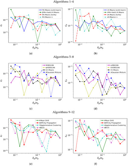
Figure 3.
Synthetic system: Relative errors in frequency, (a,c,e) and in growth rate, (b,d,f) with different clustering algorithms (1–4 in (a,b), 5–8 in (c,d), 9–12 in (e,f)).
We consider first the error behavior with increasing agglomeration level . From the comparison of Figure 3a,c,e, algorithms 1–2, 5–7, 11 and 12 offer lower error in frequency for most of the considered. Figure 3b,d,f compare the relative error for the growth rate: algorithms 1, 6, 11 and 12 show the lower errors in frequency for most of the range considered.
Not only the error behavior with is considered; the computational cost of applying DMD on a spatially agglomerated database has also been studied. The results are summarized in Figure 4. For this very simple testcase, we observe that performing agglomeration is always more expensive than handling the whole database directly: the penalty incurred in identifying the clusters overcomes the cost of the DMD on the original database. However, as we shall see in next sections, this will not be the case for more realistic flow databases. And yet, several useful lessons can be obtained from Figure 4. The first of those lessons is that using DMD at agglomeration levels close to unity does not bring any advantage, as the agglomeration procedure with many centers is typically very expensive. Another observation is that not all the agglomeration techniques bring a computational benefit: see for example, techniques 7–10: the temporal consumption is very high and practically independent from . Among the techniques that actually bring an advantage, the K-means++ technique is systematically the fastest one, despite is not the one with lower errors (cf. Figure 3). Note also how, for large agglomeration levels, the scikit-learn implementation of K-means is more efficient than the Scipy implementation. Mini-batch K-means is always cheaper than standard K-means. Finally, observe how DBSCAN, HDBSCAN, Gaussian Mixture and Agglomerative Clustering techniques present a practically uniform time consumption.
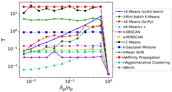
Figure 4.
Synthetic system: Average time consumption (in seconds) for different clustering algorithms.
A final comment, which will be further elaborated in Section 3.2 and Section 3.3, concerns the irregular behaviour of the error when the number of clusters changes. Although it is somehow anticipated that the error would increase when lowering , one can observe how this increment is not uniform and presents oscillations, Figure 3. Given a predefined number of clusters , different spatial agglomeration techniques lead to different cluster distributions. Those techniques that distribute the clusters into regions relevant for the underlying physical phenomena will determine more accurate frequencies/growth rates and experience lower error sensitivities.
The previous conclusions are summarized in Table 2. In order to give a fair as possible evaluation of how the different spatial agglomeration techniques considered affect the DMD analysis, the three indicators considered so far (the relative errors in frequency and growth rate and the time consumption T) are collapsed into a single number, the mark of the algorithm. Since we need to balance two goals that may compete with each other, that is, providing a sound description of the physics encoded into the database at a reduced computational cost, we have priorized the accuracy over the and efficiency: accordingly, we gauge the accuracy in frequency/temporal growth with up to 2 points both, whereas we assign the time consumption a maximum mark of 1.
Table 2.
Synthetic system: performance of the different clustering algorithms. Marks: for , mark = 2 if , mark=1 if , otherwise mark = 0; for , mark = 2 if , mark=1 if , otherwise mark = 0; for T, mark = 1 if for , otherwise mark = 0.
From Table 2, we identify seven algorithms with a mark equal or above 4. Note how C-means (algorithm 7) achieves its mark solely because its behavior in error; its potential for temporal savings is very low, see Figure 3. Accordingly, we choose six algorithms for further testing with more realistic flow databases. These algorithms are: scikit-learn K-means (algorithm 1), Mini-batch K-means (2), DBSCAN (5), HDBSCAN (6), Gaussian Mixture (8) and Agglomerative Clustering (11).
3.2. Two-Dimensional Cylinder Flow at
The 2D flow around the cross-section of an infinitely long cylinder is a typical configuration which has been extensively studied by the fluid dynamics community. DMD practitioners are not an exception, see for example, References [13,20]. Since this flow presents a Hopf bifurcation occurring at , conditions slightly above this critical value are interesting: they evince a laminar yet rich behavior, including unsteady vortex shedding, see Figure 5. In this work we consider, following Reference [20], a flow. The flow is periodic, with dominant frequency . This corresponds to a Strouhal number of , which is consistent with the correlations in Reference [51].
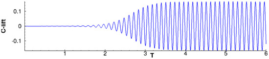
Figure 5.
cylinder flow: Evolution of lift coefficient from equilibrium steady solution to the limit cycle.
Temporally equispaced snapshots corresponding to a 2D flow around a cylinder have been generated by the DLR TAU code, a 2nd order finite volume flow solver [52]. For this data sequence, and the total non-dimensional simulation time is . The size (i.e., the number of DoFs) of the snapshots is = 36,474, and the total number of snapshots is 2400. The limit circle stage () is considered in the analyses to be presented next; this implies that the database considered consists of snapshots.
As a first measure, fast Fourier transform (FFT) was applied to the coefficient in an attempt to identify relevant frequencies present in the data, see Figure 6. Three frequencies stand out, namely , and . The higher frequencies are, practically, integer multiples of the lower one. We will focus on these frequencies when we perform the different DMD analyses.
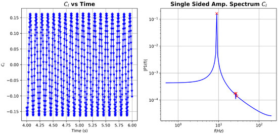
Figure 6.
cylinder flow: vs time and associated fast Fourier transform (FFT) spectrum.
Next, standard DMD has been applied to the whole data sequence . The DMD spectrum obtained is shown in Figure 7. The dynamic modes with largest are those with precisely the frequencies singled out by the FFT analysis, and supplemented with a mode with zero frequency (the temporally averaged field). Observe how 7 modes accumulate more than of the total sum of amplitude moduli. These 7 DMD modes were selected for further analysis, see their corresponding frequencies, growth ratios and spatial support in Figure 8.
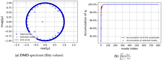
Figure 7.
cylinder flow: Dynamic Mode Decomposition (DMD) spectrum.
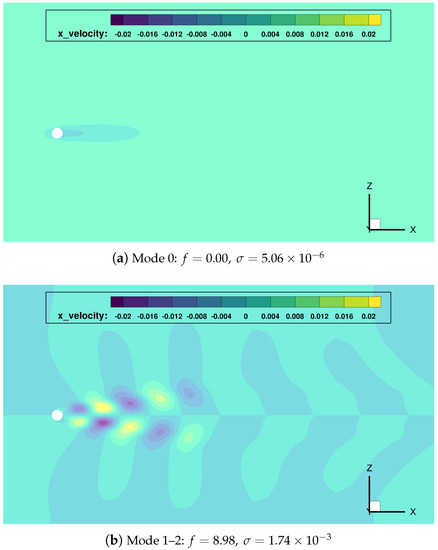
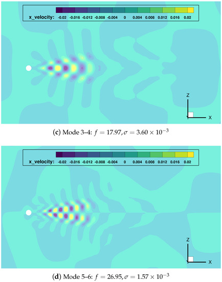
Figure 8.
cylinder flow: most relevant DMD modes, and corresponding frequencies and growth rates.
Once gain, the mode indexed as 0 () represents the temporal average of the data sequence. The main frequency mode pair (indexes 1–2) shows a growth rate close to zero, which implies it has a persistent nature in time (quasi-stability). Modes with double and triple frequency modes (pairs 3–4 and 5–6) are also found.
The modes singled out both from the FFT and the standard DMD analyses will be used to assess the sensitivity and robustness of the clustering methods selected in Section 3.1. In order to provide a comparison that is simultaneously as complete and as thorough as possible, we will consider agglomeration ratios ranging from to of the = 36,474 points in the flow field.
We assess the behavior of the spatial clustering algorithms by defining an indicator accounting for the error incurred in the determination of the 4 relevant frequencies identified by FFT (the continuous signal and the first three integer multiples of ). This indicator can be written, in normalized form, as:
where and groups the frequencies (recall that ). Taking into account that the temporal growth rate of the top modes should be practically zero, a similar quantity can be defined for the normalized error of the growth rate:
with are the growth rate corresponding to the 4 key frequencies. Assisted by these two error indicators, we perform DMD analyses on the spatially clustered cylinder flow database. Again, the error level and time consumption data presented have been obtained by averaging data from 10 different realizations. The outcome of this study regarding error behavior and computational benefit is summarized in Figure 9 and Figure 10, respectively.
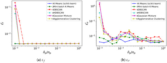
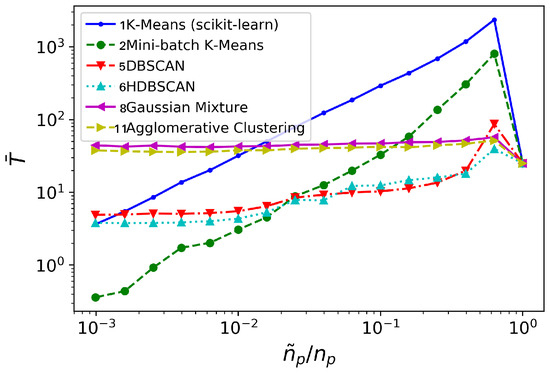
Figure 10.
cylinder flow: time invested (in seconds), for different clustering algorithms (averaged over 10 realizations).
In this case, all the methods considered behave similarly with regard to frequency error level, see Figure 9a: it remains low and practically constant for most of the spatial agglomeration levels . Mini-batch K-means behaves marginally better for the lowest cases. The growth rate error turns to be more sensitive to reductions in , see Figure 9b. No method is clearly superior to the others. However, both K-means and Mini-batch K-means provide growth rate error levels slightly lower and more uniform than the rest.
The major differences are visible from the comparison of time consumption, see Figure 10. Again, Gaussian Mixture and Agglomerative Clustering a time consumption practically insensitive to : they do not bring any computational advantage. Contrarily to the oversimplified synthetic flow considered in Section 3.1, for this testcase both DBSCAN/HDBSCAN do provide a computational advantage over the standard DMD analysis: DBSCAN/HDBSCAN bring temporal savings for . The K-means and Mini-batch K-means algorithms need higher reduction levels -respectively, and - before they offer computational savings over standard DMD analysis. However, K-means becomes competitive with DBSCAN/HDBSCAN at the lowest levels of considered; Mini-batch K-means, on the contrary, becomes competitive beyond .
In view of the previous discussion, we choose Mini-batch K-means and HDBSCAN to be tested on the turbulent channel flow problem considered in Section 3.3. Regarding the pair Gaussian Mixture/Agglomerative Clustering, they showed very similar performance. Taking into consideration the higher time and memory complexities of Agglomerative Clustering, we will favor the Gaussian Mixture method in Section 3.3.
Finally, the spatial distribution of the points selected by the clustering algorithms considered, see Figure 11, can help to explain the different error curves shown in Figure 9. Since the pairs K-means/Mini-batch K-means, DBSCAN/HDBSCAN and Gaussian Mixture/Agglomerative clustering offer similar distributions, we will only show results for the first member of the couple. Observe how K-means locates all the surviving nodes inside the Kármán vortex street, Figure 11a; this can can explain the smoother error behavior for the growth rate in Figure 9. Indeed, even for very low most of the clusters are located where the unsteady physics is involved. For the same spatial agglomeration level, DBSCAN distributes the nodes in a seemingly more random fashion, although most of them are still located in the vortex street region, see Figure 11b. This could be behind the higher error sensitivity and the ultimate deterioration once becomes excessively low. Finally, Figure 11c,d show the cluster distribution provided by Gaussian Mixture for two different levels: even with enough points within the vortex street, too many points far from the key flow zone can detrimentally affect the accuracy of the results obtained.

Figure 11.
cylinder flow: The distribution of centroids/cores from different clustering algorithms, with spatial reduction .
From this analysis, we conclude that -for a given agglomeration level - the more centroids/clusters are located in the physical features (in this case, the wake region), the higher accuracy and the lower sensitivity of the results obtained . Conversely, inspection of centroid/cluster distribution and its sensitivity to changes in might be leveraged to identify those locations most relevant for the physical phenomena investigated.
3.3. The Turbulent Channel Flow
We finally investigate the performance of the DMD method applied to a turbulent channel flow database with [31] when it is spatially agglomerated using the clustering algorithms described in Section 3.2.
The turbulent database considered has been computed by an incompressible DNS solver [53]. The code follows the paradigm introduced in Reference [54]: it solves for the wall-normal components of velocity v and vorticity . This quantities are Fourier-transformed (dealiased using the 2/3 rule) along the homogeneous directions, and discretized using explicit compact finite-differences along the wall normal direction. Both the streamwise u and spanwise w velocity components are retrieved using the continuity equation with the relation . Time integration is accomplished by an explicit third order, low-storage Runge–Kutta method, combined with an implicit second-order Crank–Nicolson scheme [55]. The simulations have been conducted under the assumption of constant flow rate. The database characteristics are summarized in Table 3. In total, 1200 flow snapshots were stored, separated in time by .
Table 3.
turbulent channel flow: database characteristics.
We will consider the temporal sequence formed by the Reynolds shear stress fields, . Following Reference [32], a simplified database that still represents the turbulent physics is obtained by removing every other point along the homogeneous x and z directions and retaining only either the lower or upper half of the domain. The resulting database, with = 117,504 and , is still large enough to pose a tough challenge for most workstations.
Since the turbulent channel flow is a multi-scale, statistically stationary phenomenon, a DMD study of the isolated modes identified is less informative than for the cylinder flow. We show nevertheless the Ritz values obtained for the full sample DMD in Figure 12a. Note how most modes lie near the locus . This is in accordance with the statistically stationary nature of the flow (see also References [19,32]). DMD analysis of the spatially agglomerated database behave in a similar way: Figure 12b shows the Ritz values for the DMD on the spatially agglomerated database using Mini-batch K-means. Ritz spectra using other agglomeration techniques do not change appreciably, and hence are not included here.
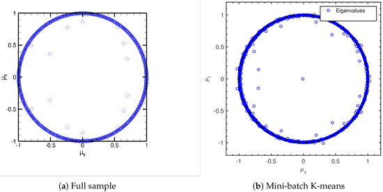
Figure 12.
turbulent channel flow: Ritz values.
The DMD method is applied to reduced databases obtained processing the original database using Mini-batch K-means, HDBSCAN and Gaussian Mixture with (i.e., or . A reduced database formed by randomly choosing spatial points is also considered, for comparison.
Figure 13 compares the profiles obtained from Equation (6) against the DNS profile. Observe how a reasonably good reconstruction of the DNS profile is obtained for all the methods selected.
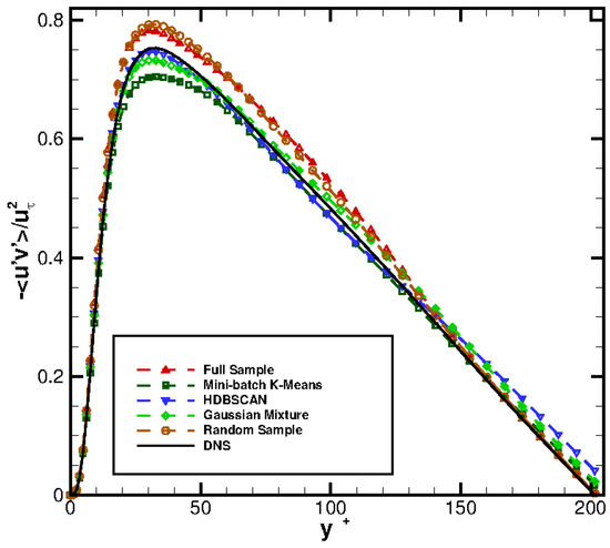
Figure 14 presents the vertical distribution of the clusters selected by the different agglomeration strategies followed. Remarkably, Gaussian Mixture and random selection retrieve, in this case, very similar distribution: this explains the similar performance shown by both methods. The Mini-batch K-means algorithm places slightly less clusters in the bin , while indicates that more clusters should be located in the bin . Finally, the HDBSCAN method finds also a cluster distribution similar to those of Gaussian Mixture/random selection. However, HDBSCAN brings a marginal improvement in the profile, see Figure 13.
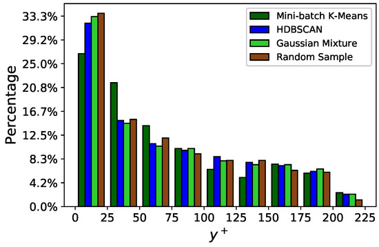
Figure 14.
turbulent channel flow: distribution of centroids along for different agglomeration strategies.
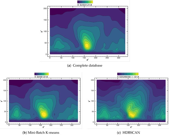
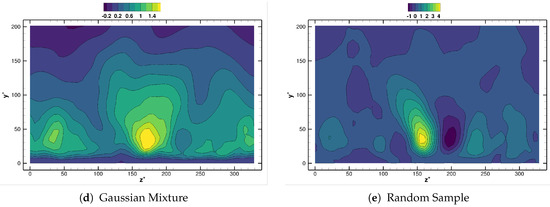
Differences between methods are more remarkable when we investigate the spanwise structure of the reconstructed Reynolds stress field, as the near wall cycle is strongly determined by features with characteristic spanwise wavelength units, see Reference [19]. Figure 15 compares for the different agglomeration strategies considered, using Equations (6) and (12). Contour levels in Figure 15 have been chosen on purpose, as this indicates how well the reconstructed flow fields respect the underlying physical flow. One strong indication of inconsistencies being present in the reconstruction is precisely the obtention of fields with improper maximum/minimum bounds. Observe how the reconstructed field from the Mini-batch K-means, in Figure 15b, is nearly indistinguishable from that one provided by DMD on the original database, Figure 15a. The field provided by the HDBSCAN method follows also closely the original results, Figure 15c. The isolines however are distributed in a range slightly narrower than the reference case. The results using Gaussian Mixture follow, overall, the reference data, though a small region with the wrong sign is apparent near the center of the channel, see Figure 15d. Finally, the field obtained with random selection of the centroids differs greatly from the reference one, and even the sign of the reconstruction is wrong in a portion of the near wall region, Figure 15e. This confirms the conclusions obtained from the cylinder case, namely that agglomeration algorithms from the K-means and DBSCAN families lead to more faithful reduced representations of the original flow data.
4. Conclusions
Dynamic mode decomposition (DMD) techniques are prominent feature identification methods in the field of fluid dynamics. Provided that a sequence of experimental measurements or numerical solutions -data snapshots- is available and assembled as a data matrix , the DMD method is capable of identifying features that evolve in time according to the complex exponential and with spatial support . Since the analysis of a complex flow field requires, in general, long temporal sequences (large N) of well resolved data (large ), the memory footprint to accomplish a DMD analysis can easily become prohibitively large.
In this contribution we have explored one of several possible avenues to alleviate the computational cost associated to DMD analysis: following Reference [30], we have investigated how the principled reduction of the data matrix using spatial agglomeration techniques affects the quality of the results that DMD can obtain.
Since typically , we have argued how spatial agglomeration of the data matrix —that is, clustering along its leading dimension- brings potentially larger reductions in computational effort. Therefore, a dozen different clustering algorithms—commonly used in the unsupervised machine learning area—have been applied to three testcases, encompassing different flow regimes: a synthetic flow field, a flow around a cylinder cross section, and a turbulent channel flow. The performance of the clustering techniques has been measured concerning not only the computational performance, but also the accuracy of the results retrieved.
In our study on the simple synthetic field we have focused on the error levels in frequency and growth error determination, together with the evaluation of temporal saving. A first observation is that, for this very simple case, the cost of applying DMD directly on the full database is always lower than the cost of the spatial agglomeration added to the DMD analysis on the reduced database; this tendency is reverted for more realistic databases, for example, the cylinder flow. Another outcome derived from the synthetic jet case is the possibility of classify the algorithms according to the error level in frequency and growth rate. As an outcome of this study, we have been able to discard six out of the twelve clustering techniques.
From the study conducted on the cylinder flow, several conclusions derive. First, in this realistic testcase, some clustering techniques do bring a computational advantage. The DBSCAN/HDBSCAN techniques are capable to provide computational savings already for relatively large agglomeration levels . However, for aggresive agglomeration, and below, Mini-batch K-means offers the lowest time consuptions, well below the other methods. The cluster initialization strategy that distinguishes Mini-batch from classical K-means really pays off in this case. Finally, we have been unsuccessful in obtaining appreciable computational savings neither from Gaussian Mixture nor from Agglomerative Clustering.
Regarding the error behavior, most of the techniques provide comparable error levels in frequency are concerned; if only, Mini-batch K-means offers low errors in all the agglomeration range considered. As for the errors in growth rate, no method clearly outperforms the others. However, both K-means and Mini-batch K-means provide growth rate error levels slightly lower than the rest.
Finally, the turbulent channel flow field at has been considered. Direct Numerical Simulation has been employed to generate the flow database used in our experiments. Mini-batch K-means, HDBSCAN and Gaussian Mixture, together with random selection of the points retained have been considered; in every case an agglomeration level of has been enforced. Surprisingly, and at least for this case, Gaussian Mixture has been found to provide results similar to those obtained by random selection of the points retained. HDBSCAN and Mini-batch K-means offer comparable results.
In view of the previous discussion, we conclude that it is worth to perform spatial agglomeration on databases that are to be analysed with dynamic mode decomposition: there is potential for savings in computational time while the errors incurred are relatively low. More specifically, it would seem that DBSCAN/HDBSCAN would be the method to be used if only relatively high agglomeration levels are affordable. On the contrary, Mini-batch K-means seems to be the method of choice whenever high agglomeration is enforced. Despite Mini-batch K-means and standard K-means offer very similar results, the former should be always used in favor of the latter, as the differences in time consumption can be very high.
Author Contributions
Conceptualization, B.L., J.G.-M. and E.V.; software, B.L.; validation, B.L., J.G.-M.; investigation, B.L., J.G.-M. and E.V.; resources, E.V. and Y.Z.; writing—original draft preparation, B.L., J.G.-M.; writing—review and editing, B.L., J.G.-M., E.V.; funding acquisition, E.V. and Y.Z. All authors have read and agreed to the published version of the manuscript.
Funding
This work is funded by Projects: Drag Reduction via Turbulent Boundary Layer Flow Control (DRAGY, GA-690623), 2016-2019, China-EU Aeronautical Cooperation project, co-funded by Ministry of Industry and Information Technology (MIIT), China, and Directorate -General for Research and Innovation (DG RTD), European Commission; and SIMOPAIL (Ref. RTI-2018-097075-B-100), Ministry of Innovation, Spain.Mr. B. Li was supported by the China Scholarship Council (CSC, No.201806320222).
Acknowledgments
The authors are grateful to M. Quadrio (Politecnico di Milano) for providing the DNS solver used in Section 3.3. The authors also acknowledge the computer resources, technical expertise and assistance provided by the Supercomputing and Visualization Center of Madrid (CeSViMa).
Conflicts of Interest
The authors declare no conflict of interest. The funders had no role whatsoever in the design of the study, the collection, analyses, or interpretation of data, in the writing of the manuscript, or in the decision to publish the results.
References
- Lumley, J.L. Stochastic Tools in Turbulence; Academic Press: Cambridge, MA, USA, 1970. [Google Scholar]
- Sirovich, L. Turbulence and the dynamics of coherent structures. Q. Appl. Math. 1987, 45, 561–590. [Google Scholar] [CrossRef]
- Berkooz, G.; Holmes, P.; Lumley, J. The Proper Orthogonal Decomposition in the Analysis of Turbulent Flows. Annu. Rev. Fluid Mech. 1993, 25, 539–575. [Google Scholar] [CrossRef]
- Volkwein, S. Proper Orthogonal Decomposition: Theory and Reduced-Order Modelling; Lecture Notes; University of Konstanz: Konstanz, Germany, 2013. [Google Scholar]
- Sieber, M.; Paschereit, C.O.; Oberleithner, K. Spectral proper orthogonal decomposition. J. Fluid Mech. 2016, 792, 798–828. [Google Scholar] [CrossRef]
- Towne, A.; Schmidt, O.; Colonius, T. Spectral proper orthogonal decomposition and its relationship to dynamic mode decomposition and resolvent analysis. J. Fluid Mech. 2018, 847, 821–867. [Google Scholar] [CrossRef]
- Derebail Muralidhar, S.; Podvin, B.; Mathelin, L.; Fraigneau, Y. Spatio-temporal proper orthogonal decomposition of turbulent channel flow. J. Fluid Mech. 2019, 864, 614–639. [Google Scholar] [CrossRef]
- Huang, N.; Shen, Z.; Long, S.; Wu, M.; Shih, H.; Zheng, Q.; Yen, N.C.; Tung, C.C.; Liu, H. The empirical mode decomposition and the Hilbert spectrum for nonlinear and non-stationary time series analysis. Proc. R. Soc. Lond. A Math. Phys. Eng. Sci. 1998, 454, 903–995. [Google Scholar] [CrossRef]
- Agostini, L.; Leschziner, M.A. On the influence of outer large-scale structures on near-wall turbulence in channel flow. Phys. Fluids 2014, 26. [Google Scholar] [CrossRef]
- Altıntaş, A.; Davidson, L.; Peng, S.H. A new approximation to modulation-effect analysis based on empirical mode decomposition. Phys. Fluids 2019, 31, 025117. [Google Scholar] [CrossRef]
- Schmid, P. Dynamic mode decomposition of numerical and experimental data. J. Fluid Mech. 2010, 656, 5–28. [Google Scholar] [CrossRef]
- Rowley, C.; Mezić, I.; Bagheri, S.; Schlatter, P.; Henningson, D. Spectral analysis of nonlinear flows. J. Fluid Mech. 2009, 641, 115–127. [Google Scholar] [CrossRef]
- Chen, K.; Tu, J.; Rowley, C. Variants of Dynamic Mode Decomposition: Boundary condition, Koopman, and Fourier Analyses. J. Nonlinear Sci. 2012, 22, 887–915. [Google Scholar] [CrossRef]
- Le Clainche, S.; Vega, J. Higher Order Dynamic Mode Decomposition. SIAM J. Appl. Dyn. Syst. 2017, 16, 882–925. [Google Scholar] [CrossRef]
- Dawson, S.; Hemati, M.; Williams, M.; Rowley, C. Characterizing and correcting for the effect of sensor noise in the dynamic mode decomposition. Exp. Fluids 2016, 75. [Google Scholar] [CrossRef]
- Duke, D.; Soria, J.; Honnery, D. An error analysis of the Dynamic Mode Decomposition. Exp. Fluids 2012, 52, 529–542. [Google Scholar] [CrossRef]
- Schmid, P.; Violato, D.; Scarano, F. Decomposition of time-resolved tomographic PIV. Exp. Fluids 2012, 52, 1567–1579. [Google Scholar] [CrossRef]
- Le Clainche, S.; Vega, J.; Soria, J. Higher Order Dynamic Mode Decomposition of noisy experimental data: The flow structure of a zero-net-mass-flux jet. Exp. Therm. Fluid Sci. 2017, 88, 336–353. [Google Scholar] [CrossRef]
- Cassinelli, A.; de Giovanetti, M.; Hwang, Y. Streak instability in near-wall turbulence revisited. J. Turbul. 2017, 18, 443–464. [Google Scholar] [CrossRef]
- Kou, J.; Zhang, W. An improved criterion to select dominant modes from Dynamic Mode Decomposition. Eur. J. Mech. B/Fluids 2017, 62, 109–129. [Google Scholar] [CrossRef]
- Grenga, T.; MacArt, J.; Mueller, M. Dynamic Mode Decomposition of a direct numerical simulation of a turbulent premixed planar jet flame: Convergence of the modes. Combust. Theory Model. 2018, 22, 1–17. [Google Scholar] [CrossRef]
- Le Clainche, S.; Izbassarov, D.; Rosti, M.; Brandt, L.; Tammisola, O. Coherent structures in the turbulent channel flow of an elastoviscoplastic fluid. J. Fluid Mech. 2020, 888, A5. [Google Scholar] [CrossRef]
- Kutz, J.N.; Brunton, S.L.; Brunton, B.W.; Proctor, J.L. Dynamic Mode Decomposition: Data-Driven Modeling of Complex Systems; SIAM: Philadelphia, PA, USA, 2016. [Google Scholar]
- Sayadi, T.; Schmid, P. Parallel data-driven decomposition algorithm for large-scale datasets: With application to transitional boundary layers. Theor. Comp. Fluid Dyn. 2016, 30, 415–428. [Google Scholar] [CrossRef]
- Bistrian, D.; Navon, I. Randomized dynamic mode decomposition for nonintrusive reduced order modelling. Int. J. Numer. Methods Fluids 2017, 112, 3–25. [Google Scholar] [CrossRef]
- Erichson, N.; Mathelin, L.; Brunton, S.; Kutz, J. Randomized Dynamic Mode Decomposition. arXiv e-Prints 2018, arXiv:1702.02912. [Google Scholar] [CrossRef]
- Halko, N.; Martinsson, P.G.; Tropp, J. Finding Structure with Randomness: Probabilistic Algorithms for Constructing Approximate Matrix Decompositions. SIAM Rev. 2011, 53, 217–288. [Google Scholar] [CrossRef]
- Brunton, S.; Proctor, J.; Tu, J.; Kutz, J. Compressed sensing and dynamic mode decomposition. J. Comput. Dyn. 2015, 2, 165–191. [Google Scholar] [CrossRef]
- Erichson, N.B.; Brunton, S.; Kutz, J.N. Compressed dynamic mode decomposition for background modeling. J. Real-Time Image Process. 2019, 16, 1479–1492. [Google Scholar] [CrossRef]
- Guéniat, F.; Mathelin, L.; Pastur, L.R. A Dynamic Mode Decomposition approach for large and arbitrarily sampled systems. Phys. Fluids 2015, 27, 025113. [Google Scholar] [CrossRef]
- Quadrio, M.; Frohnapfel, B.; Hasegawa, Y. Does the choice of the forcing term affect flow statistics in DNS of turbulent channel flow? Eur. J. Mech. B/Fluids 2016, 55, 286–293. [Google Scholar] [CrossRef]
- Garicano-Mena, J.; Li, B.; Ferrer, E.; Valero, E. A composite dynamic mode decomposition analysis of turbulent channel flows. Phys. Fluids 2019, 31, 115102. [Google Scholar] [CrossRef]
- Mezić, I. Analysis of fluid flows via spectral properties of the Koopman operator. Annu. Rev. Fluid Mech. 2013, 45, 357–378. [Google Scholar] [CrossRef]
- Saad, Y. Numerical Methods for Large Eigenvalue Problems; Manchester University Press: Manchester, UK, 1992. [Google Scholar]
- Rowley, C.; Dawson, S. Model Reduction for Flow Analysis and Control. Annu. Rev. Fluid Mech. 2017, 49, 387–417. [Google Scholar] [CrossRef]
- Jovanović, M.R.; Schmid, P.J.; Nichols, J.W. Sparsity-promoting Dynamic Mode Decomposition. Phys. Fluids 2014, 26, 024103. [Google Scholar] [CrossRef]
- Virtanen, P.; Gommers, R.; Oliphant, T.E.; Haberland, M.; Reddy, T.; Cournapeau, D.; Burovski, E.; Peterson, P.; Weckesser, W.; Bright, J.; et al. SciPy 1.0: Fundamental Algorithms for Scientific Computing in Python. Nat. Methods 2020, 17, 261–272. [Google Scholar] [CrossRef] [PubMed]
- Pedregosa, F.; Varoquaux, G.; Gramfort, A.; Michel, V.; Thirion, B.; Grisel, O.; Blondel, M.; Prettenhofer, P.; Weiss, R.; Dubourg, V.; et al. Scikit-learn: Machine Learning in Python. J. Mach. Learn. Res. 2011, 12, 2825–2830. [Google Scholar]
- Jin, X.; Han, J. K-means clustering. In Encyclopedia of Machine Learning and Data Mining; Springer: New York, NY, USA, 2017; pp. 695–697. [Google Scholar]
- Sculley, D. Web-scale k-means clustering. In Proceedings of the 19th International Conference on World Wide Web, Raleigh, NC, USA, 26–30 April 2010; ACM: New York, NY, USA, 2010; pp. 1177–1178. [Google Scholar]
- Arthur, D.; Vassilvitskii, S. K-means++: The advantages of careful seeding. In Proceedings of the Eighteenth Annual ACM-SIAM Symposium on Discrete Algorithms, New Orleans, LA, USA, 7–9 January 2007; Society for Industrial and Applied Mathematics: Philadelphia, PA, USA, 2007; pp. 1027–1035. [Google Scholar]
- Ester, M.; Kriegel, H.P.; Sander, J.; Xu, X. A Density-Based Algorithm for Discovering Clusters in Large Spatial Databases with Noise; AAAI Press: Palo Alto, CA, USA, 1996; pp. 226–231. [Google Scholar]
- Schubert, E.; Sander, J.; Ester, M.; Kriegel, H.P.; Xu, X. DBSCAN revisited, revisited: Why and how you should (still) use DBSCAN. ACM Trans. Database Syst. 2017, 42, 19. [Google Scholar] [CrossRef]
- Campello, R.; Moulavi, D.; Sander, J. Density-based clustering based on hierarchical density estimates. In Proceedings of the Pacific-Asia Conference on Knowledge Discovery and Data Mining, Gold Coast, QLD, Australia, 14–17 April 2013; Springer: Berlin/Heidelberg, Germany, 2013; pp. 160–172. [Google Scholar]
- Bezdek, J.C. Pattern Recognition with Fuzzy Objective Function Algorithms; Springer Science & Business Media: Berlin, Germany, 2013. [Google Scholar]
- Pinto, R.; Engel, P. A fast incremental Gaussian Mixture model. PLoS ONE 2015, 10, e0139931. [Google Scholar] [CrossRef]
- Li, X.; Zhong, Z.; Wu, J.; Yang, Y.; Lin, Z.; Liu, H. Expectation-Maximization Attention Networks for Semantic Segmentation. In Proceedings of the 2019 IEEE/CVF International Conference on Computer Vision (ICCV), Seoul, Korea, 27 October–2 November 2019; pp. 9166–9175. [Google Scholar]
- Comaniciu, D.; Meer, P. Mean shift: A robust approach toward feature space analysis. IEEE Trans. Pattern Anal. Mach. Intell. 2002, 24, 603–619. [Google Scholar] [CrossRef]
- Frey, B.J.; Dueck, D. Clustering by Passing Messages Between Data Points. Science 2007, 315, 972–976. [Google Scholar] [CrossRef]
- Zhang, T.; Ramakrishnan, R.; Livny, M. BIRCH: An efficient data clustering method for very large databases. In ACM Sigmod Record; ACM: New York, NY, USA, 1996; Volume 25, pp. 103–114. [Google Scholar]
- Roshko, A. On the Development of Turbulent Wakes from Vortex Streets; TN 1191; NACA: Washington, DC, USA, 1954. [Google Scholar]
- Schwamborn, D.; Gerhold, T.; Heinrich, R. The DLR TAU-code: Recent applications in research and industry. In Proceedings of the ECCOMAS CFD Conference, Egmond aan Zee, The Netherlands, 5–8 September 2006. [Google Scholar]
- Luchini, P.; Quadrio, M. A Low-cost Parallel Implementation of Direct Numerical Simulation of Wall Turbulence. J. Comput. Phys. 2006, 211, 551–571. [Google Scholar] [CrossRef]
- Kim, J.; Moin, P.; Moser, R. Turbulence statistics in fully developed channel flow at low Reynolds number. J. Fluid Mech. 1987, 177, 133–166. [Google Scholar] [CrossRef]
- Moser, R.; Kim, J.; Mansour, N. Direct numerical simulation of turbulent channel flow up to Reτ = 590. Phys. Fluids 1999, 11, 943–945. [Google Scholar] [CrossRef]


© 2020 by the authors. Licensee MDPI, Basel, Switzerland. This article is an open access article distributed under the terms and conditions of the Creative Commons Attribution (CC BY) license (http://creativecommons.org/licenses/by/4.0/).