A Novel Algebraic Stress Model with Machine-Learning-Assisted Parameterization

Abstract

Reynolds-stress closure modeling is critical to Reynolds-averaged Navier-Stokes (RANS) analysis, and it remains a challenging issue in reducing both structural and parametric inaccuracies. This study first proposes a novel algebraic stress model named as tensorial quadratic eddy-viscosity model (TQEVM), in which nonlinear terms improve previous model-form failure due to neglection of nonlocal effects. Then a data-driven regression model based on a fully-connected deep neural network is designed to determine the TQEVM coefficients. The well-trained data-driven model using high-fidelity direct numerical simulation (DNS) data successfully learned the underlying input-output relationships, further obtaining spatial-dependent optimal values of these coefficients. Finally, detailed validations are made in wall-bounded flows where nonlocal effects are expected to be significant. Comparative results indicate that TQEVM provides improvements both for the stress-strain misalignment and stress anisotropy, which are clear advantages over linear and quadratic eddy-viscosity models. TQEVM extends to the scope of resolution to the wall distance $y^{+}\approx 9$ as well as provides a realizable solution. RANS simulations with TQEVM are also carried out and the obtained mean-flow quantities of interest agree well with DNS. This work, therefore, results in a high-fidelity representation of Reynolds stresses and contributes to further understanding of machine-learning-assisted turbulence modeling and regression analysis.

1. Introduction

There are many kinds of turbulence phenomena in energy engineering, e.g., the wake meandering. To understand these complicated flow behavior, turbulence simulation and modeling is an important and useful tool, which has been extensively investigated and comprehensively reviewed [1,2,3,4,5]. Although more accurate scale-resolving simulations, e.g., large-eddy simulation (LES) and direct numerical simulation (DNS), are increasingly popular, Reynolds-averaged Navier-Stokes (RANS) analysis remains a widely used option in computational fluid dynamics due to its efficiency [3] and is expanding into new stages [5,6]. However, RANS analysis relies heavily on accurate closure model for Reynolds stresses, including structural (model-form) and parametric (model-parameter) adequate representations of real physics.

Various Reynolds-stress closures have been proposed. Most popular are still the linear eddy-viscosity models (EVMs), mainly including the Spalart-Allmaras model [7], SST k-ω model [8] and Realizable k-$ϵ$ model [9]. A number of improvements have been made on these models aiming at improving sensitivity to curvature and/or rotation effects, such as introducing corrections into the eddy viscosity equation [10], the dissipation rate equation [11], the specific dissipation rate equation [12], and introducing corrections into eddy-viscosity coefficient [12,13]. However, none of the essential changes occur in the baseline framework of closure modeling. Obviously, the variant closure coefficients cannot improve the inherent limitations due to the underlying model-form inaccuracy rooted in Boussinesq hypothesis.

Linear stress-strain relationship origins from the Boussinesq hypothesis that turbulence react locally to the changes of mean-flow behavior in equilibrium flows. However, that is not really the case. In most turbulent flows, there exists a large misalignment in stress-strain response which has been repeatedly confirmed with high-fidelity DNS investigation [14,15,16]. In view of pressure-strain correlations in the exact Reynolds-stress transport equations, the stress-strain misalignment is theoretically generated from the nonlocal response of the pressure to the entire flow field through Green’s functions [17]. As a result, the in-phase type EVMs certainly experience failure, especially in flows with strong spatial inhomogeneity (e.g., rotation/curvature [10,18], three-dimensionality [19], secondary-flow [20], etc.). These flow effects make changes in the mean shear (i.e., spatial inhomogeneity) and turbulence structures [21,22,23], further enhancing nonlocality on the stress-strain misalignment. Hamlington and Dahm [24] also observed that EVMs over-predict shear stresses and give inappropriate isotropic normal stresses even in simple parallel shear flows, and further explained the failure as a neglection of nonlocal effects. Edeling, et al. [25] argued that the failure of EVMs is attributed to the lack of physical interpretation of stress-strain misalignment. Although recent progress in representation of shear-stress-strain misalignment (see, e.g., [26,27]) has been made by three-equation EVMs (as an aside, misrepresentation of real physics [19,28] and increasing computational cost), these variants still fail in predictions of normal stresses, which are closely related to turbulent structures in channel flows [29] and secondary motions in non-circular ducts [30]. Model-form inaccuracy cannot be reduced by corrections of model-parameter inaccuracy.

Nonlinear eddy-viscosity models (NLEVMs), referring to the second class of RANS closure in Figure 1b, is a generalization of the Boussinesq hypothesis, which was first proposed by Lumley [31] and investigated in a systematic way by Pope [32]. A step forward over EVMs is that NLEVMs have the potential to improve normal stresses through added nonlinear terms (e.g., a k-ω² model of Wilcox and Rubesin [33]). However, no further improvements in shear stresses (same as EVMs) are obtained in most flows. According to RANS equations, the predictions of normal stresses also depend on the axial-flow motion which is controlled by the dominant shear stresses. Therefore, the key to improvements at a given NLEVM model-form returns to model-parameter optimization as EVMs do. At this point, this problem is not easy to settle down through conventional regression analysis due to following reasons (more details in Section 3): (i) lack of prior knowledge about how to select features as arguments, (ii) strong nonlinearity, resulting in difficulty in design of functional forms, (iii) high-dimensionality and computational cost, and (iv) spatial independence of the obtained coefficients. For quadratic eddy-viscosity models (QEVMs) commonly used, for instance, different values of closure coefficients [34,35,36,37,38] were introduced, however, no further improvements are obtained in most flows.

Recently, machine learning algorithms may take a breakthrough for turbulence modeling. Weatheritt and Sandberg [39] employed gene expression programming to calibrate the closure coefficients of QEVMs. Zhu, et al. [40] approximated the eddy-viscosity coefficient only existed in EVMs with a single-layer neural network and tested by flows around simple airfoils. The former obtained algebraic models with explicit analytical forms, while the latter is a data-driven model. These machine learning-based regression analyses are successful in reducing model-parameter inaccuracy. Nevertheless, normal stresses cannot be predicted correctly using the model trained by Zhu, et al. [40] because of the model-form inaccuracy of EVMs. Similarly, the model-form inaccuracy in QEVMs proposed by Weatheritt and Sandberg [39] leads to the fact that not all dominant shear stresses can be predicted correctly with the only sharing closure coefficient, thus resulting in failure in flows where there are different misalignments between shear components and corresponding mean strain (e.g., secondary flow [20] and three-dimensional boundary layer [41]). Therefore, an adequate model-form representation of Reynolds stress is critical before using machine-learning-assisted regression analysis. Ling, et al. [42] adopts a more general form of NLEVMs based on 10 independent tensor bases from representation theory and then learns the closure coefficients using 5 invariants as inputs of the neural networks. Testing results show that embedded invariance properties can improve significantly the performance of the neural networks. Besides, Wang, et al. [43] applied machine learning to directly predict the Reynolds stresses discrepancies (corresponding to nonlinear terms in NLEVMs) compared to the truth, forming implicit algebraic NLEVMs. The main drawbacks of these implicit models are poor interpretability of black-box models, numerical convergence and transfer (or generalization) to another flow configuration [44]. Edeling, Iaccarino, and Cinnella [25] also argued that the complex input-output mapping of black-box models are unable to increase confidence. A more comprehensive overview of data-driven turbulence modeling has been presented in Refs. [5].

NLEVMs also can be derived by Reynolds-stress transport models (RSTMs), referring to the third class of RANS closure in Figure 1b, and examples are models mentioned above (e.g., k-ω² model of Wilcox and Rubesin [33], and that of Hamlington and Dahm [24]). RSTMs are rarely used in engineering due to the high computational cost and complexity, and not further reviewed here (refer to [2,3,4]). Therefore, it is concluded that NLEVMs are increasingly popular for RANS-based turbulence modeling, especially in the age of data.

This work seeks to reduce both structural and parametric inaccuracies with a novel proposed NLEVM and machine-learning-assisted parameterization. The remainder of this article is organized as follows: In Section 2, we develop a novel algebraic stress-strain relationship as RANS closures, in which nonlinear terms can reduce model-form inaccuracy due to the stress-strain misalignment. Then a machine learning strategy is applied to the symbolic regression of the coefficients in the closure proposal in Section 3. Section 4 covers a prior validation in testing datasets and a posterior numerical simulation to evaluate model performance and followed by conclusions in Section 5.

2. A Novel Stress Closure Proposal

It is increasingly important to develop an adequate model-form representation of real physics, which helps to capture missed features in traditional models. As mentioned above, the failure of EVMs and NLEVMs is mainly attributed to stress-strain misalignment due to nonlocal effects [24,25]. Spalart [2] also argued that modeled physics should be enhanced by nonlocal models which are categorized into two types: (i) models incorporating a scalar involving entire information, e.g., the wall distance (although it is not an invariant) in the Spalart-Allmaras model [7], and (ii) models involving high-order derivatives of the mean velocity. Here, to consider nonlocal effects with high accuracy, a stress closure model is proposed, which should fall into the second type model.

The key idea here is to consider nonlocal effects on the anisotropy evolution of the Reynolds stress tensor by constructing velocity fluctuations with nonlocal velocity gradients. Assume that the velocity increment between every two locations contributes to velocity fluctuations with a two-point correlation weight coefficient.

At an instantaneous time, the increment of flow velocity between two locations $\widehat{x}$ and $x$ can be expressed in terms of a Taylor series expansion with respect to the current location $x$,

$$u_i(\widehat{x},t)-u_i(x,t)=r_m \frac{\partial u_i}{\partial x_m}{|}_x+\frac{1}{2}{r}_p{r}_q \frac{{\partial }^2{u}_i}{\partial x_p\partial x_q}{|}_x+\dots +\frac{1}{n!}(r_s{r}_t\dots )\frac{{\partial }^n{u}_i}{\partial x_s\partial x_t\dots }{|}_x$$

(1)

where $r_m\equiv {\widehat{x}}_m-x_m$.

From a physical point of view, turbulence develops as instability of shear layers, and the turbulent fluctuations are closely related to the velocity gradients. Thus, the velocity increment between two locations contributes to velocity fluctuations. The motion of fluid at any location in a turbulent flow is always influenced by the motion at other locations through the pressure field, i.e., nonlocal effects (see Appendix A). Then the contribution of velocities at other locations in the whole flow field to the velocity at a reference location can be accounted for through weight coefficients. An expression of velocity fluctuations $u_i^{\prime }$ at current location $x$ is given as

$$u_i^{\prime }(x,t)={\displaystyle \sum _{r\in \mathsf{\Lambda }}\alpha (x,t;r)\left[u_i(\widehat{x},t)-u_i(x,t)\right]}$$

(2)

where $r\equiv \widehat{x}-x$, the space $\mathsf{\Lambda }$ is taken to be theoretically infinite, and the dimensionless weight coefficient $\alpha$ represents the influence intensity of location $\widehat{x}$ on reference location $x$, varying inversely with the relative distance $r_m$.

Substituting Equation (1) into Equation (2), we obtain:

$$u_i^{\prime }(x,t)=\frac{\partial u_i}{\partial x_m}{|}_x \cdot L_m+\frac{{\partial }^2{u}_i}{\partial x_p\partial x_q}{|}_x\cdot L_{pq}^2+\dots +\frac{{\partial }^2{u}_i}{\partial x_s\partial x_t\dots }{|}_x\cdot L_{st\dots }^n,$$

(3)

where

$$L_{st\dots }^n(x,t)\equiv {\displaystyle \sum _{r\in \mathsf{\Lambda }}[\alpha (x,t;r)\frac{1}{n!}(r_s{r}_t\dots )]}.$$

(4)

The ensemble average of coefficients $\alpha$ in Equation (4) represents averaging influence intensity between two points, and thus can be defined as a function of two-point correlation of flow quantities (e.g., pressure fluctuation $p^{\prime }$), i.e.,

$$\overline{\alpha }(x,t;r)=f[R(x,t;r)/R(x,t;0)],$$

(5)

where

$$R(x,t;r)\hspace{0.17em}=\hspace{0.17em}\overline{p^{\prime }(x,t)p^{\prime }(x+r,t)}.$$

(6)

The coefficients $L_m$ in Equation (4) represent equivalent influence distances or equivalent nonlocal length scales. The ensemble averages of these coefficients are approximately equal to themselves, i.e., ${\overline{L}}_m\approx L_m$, because the summation over the whole domain nearly experiences all states in all realizations. Other coefficients in Equation (3) also hold this property.

Obviously, nonlocal effects are involved in Equation (3) along with closure coefficients. The linear expansion in Equation (3) is suitable for flows in which the variations of the velocity gradients are not too large. When very strong spatial inhomogeneity exists (e.g., a three-dimensional turbulent boundary layer), a second-order expansion may be needed. Terms up to quadratic velocity gradients in Equation (3) are sufficient for the vast majority of turbulent flows. Thus, Equation (3) reduces to:

$$u_i^{\prime }=L_m\frac{\partial u_i}{\partial x_m}+L_{pq}^2\frac{{\partial }^2{u}_i}{\partial x_p\partial x_q}.$$

(7)

Applying an ensemble average to products of any two fluctuating components in Equation (7), the corresponding form for Reynolds stress is derived and further expressed with Reynolds decomposition of the flow variables into ensemble mean and fluctuating components as:

$$\overline{u_i^{\prime }{u}_j^{\prime }}={\left(\overline{u_i^{\prime }{u}_j^{\prime }}\right)}_I+{\left(\overline{u_i^{\prime }{u}_j^{\prime }}\right)}_{II}+{\left(\overline{u_i^{\prime }{u}_j^{\prime }}\right)}_{III}+{\left(\overline{u_i^{\prime }{u}_j^{\prime }}\right)}_{IV},$$

(8)

where

$${\left(\overline{u_i^{\prime }{u}_j^{\prime }}\right)}_I=L_m{L}_n\frac{\partial {\overline{u}}_i}{\partial x_m}\frac{\partial {\overline{u}}_j}{\partial x_n}+L_m{L}_n\overline{\frac{\partial u_i^{\prime }}{\partial x_m}\frac{\partial u_j^{\prime }}{\partial x_n}},$$

(9)

$${\left(\overline{u_i^{\prime }{u}_j^{\prime }}\right)}_{II}=L_{pq}^2{L}_{kl}^2\frac{{\partial }^2{\overline{u}}_i}{\partial x_p\partial x_q}\frac{{\partial }^2{\overline{u}}_j}{\partial x_k\partial x_l}+L_{pq}^2{L}_{kl}^2\overline{\frac{{\partial }^2{u}_i^{\prime }}{\partial x_p\partial x_q}\frac{{\partial }^2{u}_j^{\prime }}{\partial x_k\partial x_l}},$$

(10)

$${\left(\overline{u_i^{\prime }{u}_j^{\prime }}\right)}_{III}=L_m{L}_{kl}^2\frac{\partial {\overline{u}}_i}{\partial x_m}\frac{{\partial }^2{\overline{u}}_j}{\partial x_k\partial x_l}+L_m{L}_{kl}^2\overline{\frac{\partial u_i^{\prime }}{\partial x_m}\frac{{\partial }^2{u}_j^{\prime }}{\partial x_k\partial x_l}},$$

(11)

$${\left(\overline{u_i^{\prime }{u}_j^{\prime }}\right)}_{IV}=L_{pq}^2{L}_n\frac{{\partial }^2{\overline{u}}_i}{\partial x_p\partial x_q}\frac{\partial {\overline{u}}_j}{\partial x_n}+L_{pq}^2{L}_n\overline{\frac{{\partial }^2{u}_i^{\prime }}{\partial x_p\partial x_q}\frac{\partial u_j^{\prime }}{\partial x_n}}.$$

(12)

The first term in Equation (9) accounts for direct effects of mean velocity gradients on the anisotropy evolution, which corresponds to the rapid part ${\mathsf{\Pi }}_{ij}^r$ relating to nonlocal effects due to variations in the mean shear (see Appendix A), the second term represents turbulence-turbulence interactions and forces the turbulence to become isotropic, which corresponds to the slow part, ${\mathsf{\Pi }}_{ij}^s$. Similar to ${\mathsf{\Pi }}_{ij}^s$, the second term can be split into a purely local contribution (i.e., $Ek{ϵ}_{ij}/ϵ$) and the remaining nonlocal part. The former plays a dominant role in the second term in Equation (9), while the latter is relatively small and can be incorporated in the first term. Equation (9) can be rewritten as

$${\left(\overline{u_i^{\prime }{u}_j^{\prime }}\right)}_I=[L_m{L}_n\frac{\partial {\overline{u}}_i}{\partial x_m}\frac{\partial {\overline{u}}_j}{\partial x_n}+(L_m{L}_n\overline{\frac{\partial u_i^{\prime }}{\partial x_m}\frac{\partial u_j^{\prime }}{\partial x_n}}-2\nu E \frac{k}{ϵ} \overline{\frac{\partial u_i^{\prime }}{\partial x_k}\frac{\partial u_j^{\prime }}{\partial x_k}})]+E\frac{k}{ϵ}{ϵ}_{ij},$$

(13)

where E is a coefficient and $ϵ$ is the dissipation rate of k. All of the terms inside the square brackets on the right side of Equation (13) represent nonlocal effects due to spatial variations in the mean shear (including local contributions of the mean shear) and the adjustment of turbulence itself.

Equation (13) can be expressed with a decomposition of the velocity gradients into symmetric and antisymmetric parts, as follows:

$$\begin{array}{ll}{\left(\overline{u_i^{\prime }{u}_j^{\prime }}\right)}_I& =B_{mn}({\overline{S}}_{im}{\overline{S}}_{jn}-\frac{1}{3}{\overline{S}}_{km}{\overline{S}}_{kn}{\delta }_{ij})\\ & +C_{mn}[{\overline{S}}_{im}{\overline{\mathsf{\Omega }}}_{jn}+{\overline{\mathsf{\Omega }}}_{im}{\overline{S}}_{jn}-\frac{1}{3}({\overline{S}}_{km}{\overline{\mathsf{\Omega }}}_{kn}+{\overline{\mathsf{\Omega }}}_{km}{\overline{S}}_{kn}){\delta }_{ij}]\\ & +D_{mn}({\overline{\mathsf{\Omega }}}_{im}{\overline{\mathsf{\Omega }}}_{jn}-\frac{1}{3}{\overline{\mathsf{\Omega }}}_{km}{\overline{\mathsf{\Omega }}}_{kn}{\delta }_{ij})+E\frac{k}{ϵ}{ϵ}_{ij}\end{array}$$

(14)

where the closure coefficients are defined as:

$$B_{mn}\equiv \frac{L_m{L}_n({\overline{S}}_{im}{\overline{S}}_{jn}+\overline{S_{im}^{\prime }{S}_{jn}^{\prime }})-2\nu E\frac{k}{ϵ} \overline{S_{ik}^{\prime }{S}_{jk}^{\prime }}}{{\overline{S}}_{im}{\overline{S}}_{jn}-\frac{1}{3}{\overline{S}}_{km}{\overline{S}}_{kn}{\delta }_{ij}},$$

(15)

$$C_{mn}\equiv \frac{L_m{L}_n({\overline{S}}_{im}{\overline{\mathsf{\Omega }}}_{jn}+{\overline{\mathsf{\Omega }}}_{im}{\overline{S}}_{jn}+\overline{S_{im}^{\prime }{\mathsf{\Omega }}_{jn}^{\prime }}+\overline{{\mathsf{\Omega }}_{im}^{\prime }{S}_{jn}^{\prime }} )-2\nu E\frac{k}{ϵ} (\overline{S_{ik}^{\prime }{\mathsf{\Omega }}_{jk}^{\prime }}+\overline{{\mathsf{\Omega }}_{ik}^{\prime }{S}_{jk}^{\prime }})}{{\overline{S}}_{im}{\overline{\mathsf{\Omega }}}_{jn}+{\overline{\mathsf{\Omega }}}_{im}{\overline{S}}_{jn}-\frac{1}{3}({\overline{S}}_{km}{\overline{\mathsf{\Omega }}}_{kn}+{\overline{\mathsf{\Omega }}}_{km}{\overline{S}}_{kn}){\delta }_{ij}},$$

(16)

$$D_{mn}\equiv \frac{L_m{L}_n({\overline{\mathsf{\Omega }}}_{im}{\overline{\mathsf{\Omega }}}_{jn}+\overline{{\mathsf{\Omega }}_{im}^{\prime }{\mathsf{\Omega }}_{jn}^{\prime }})-2\nu E\frac{k}{ϵ} \overline{{\mathsf{\Omega }}_{ik}^{\prime }{\mathsf{\Omega }}_{jk}^{\prime }}}{{\overline{\mathsf{\Omega }}}_{im}{\overline{\mathsf{\Omega }}}_{jn}-\frac{1}{3}{\overline{\mathsf{\Omega }}}_{km}{\overline{\mathsf{\Omega }}}_{kn}{\delta }_{ij}},$$

(17)

where $S_{ij}^{\prime }\equiv (\partial u_i^{\prime }/\partial x_j+\partial u_j^{\prime }/\partial x_i)/2$ and ${\mathsf{\Omega }}_{ij}^{\prime }\equiv (\partial u_i^{\prime }/\partial x_j-\partial u_j^{\prime }/\partial x_i)/2$, the closure coefficients $B_{mn}$, $C_{mn}$, and $D_{mn}$ involve nonlocal length scales $L_m$, k, $ϵ$, and/or mean strain and rotation rate tensors.

Now we discuss the last term in Equation (14). Since the dissipation is in reality anisotropic (but relatively weak), particularly close to solid boundaries, a form of ${ϵ}_{ij}$ similar to the formula proposed by Hanjalić and Launder [45] is chosen, in which the weakly anisotropic part is related to stress anisotropy modeled by linear EVMs. Thus,

$${ϵ}_{ij}=\frac{2}{3}ϵ{\delta }_{ij}+ϵ(-2\frac{{\nu }_t}{k}{\overline{S}}_{ij}).$$

(18)

Furthermore, to guarantee that the trace of $\overline{u_i^{\prime }{u}_j^{\prime }}$ is 2k, it gets E = 1 (for incompressible flows, ${\overline{S}}_{kk}$ = 0). Thus, the general formulation of Equation (14) simplifies to

$$\begin{array}{ll}{\left(\overline{u_i^{\prime }{u}_j^{\prime }}\right)}_I& =\frac{2}{3}k{\delta }_{ij}-2{\nu }_t{\overline{S}}_{ij}+B_{mn}({\overline{S}}_{im}{\overline{S}}_{jn}-\frac{1}{3}{\overline{S}}_{km}{\overline{S}}_{kn}{\delta }_{ij})\\ & +C_{mn}[{\overline{S}}_{im}{\overline{\mathsf{\Omega }}}_{jn}+{\overline{\mathsf{\Omega }}}_{im}{\overline{S}}_{jn}-\frac{1}{3}({\overline{S}}_{km}{\overline{\mathsf{\Omega }}}_{kn}+{\overline{\mathsf{\Omega }}}_{km}{\overline{S}}_{kn}){\delta }_{ij}]\\ & +D_{mn}({\overline{\mathsf{\Omega }}}_{im}{\overline{\mathsf{\Omega }}}_{jn}-\frac{1}{3}{\overline{\mathsf{\Omega }}}_{km}{\overline{\mathsf{\Omega }}}_{kn}{\delta }_{ij})\end{array}$$

(19)

A similar analysis can be applied to Equations (15)–(17). Here, the local contribution from turbulence itself to the anisotropy can be neglected due to its small contribution. Then, we obtain:

$$\begin{array}{ll}{\left(\overline{u_i^{\prime }{u}_j^{\prime }}\right)}_{II}& =B_{pqkl}(\frac{\partial {\overline{S}}_{ip}}{\partial x_q}\frac{\partial {\overline{S}}_{jk}}{\partial x_l}-\frac{1}{3}\frac{\partial {\overline{S}}_{mp}}{\partial x_q}\frac{\partial {\overline{S}}_{mk}}{\partial x_l}{\delta }_{ij})\\ & +C_{pqkl}[\frac{\partial {\overline{S}}_{ip}}{\partial x_q}\frac{\partial {\overline{\mathsf{\Omega }}}_{jk}}{\partial x_l}+\frac{\partial {\overline{\mathsf{\Omega }}}_{ip}}{\partial x_q}\frac{\partial {\overline{S}}_{jk}}{\partial x_l}-\frac{1}{3}(\frac{\partial {\overline{S}}_{mp}}{\partial x_q}\frac{\partial {\overline{\mathsf{\Omega }}}_{mk}}{\partial x_l}+\frac{\partial {\overline{\mathsf{\Omega }}}_{mp}}{\partial x_q}\frac{\partial {\overline{S}}_{mk}}{\partial x_l}){\delta }_{ij}]\\ & +D_{pqkl}(\frac{\partial {\overline{\mathsf{\Omega }}}_{ip}}{\partial x_q}\frac{\partial {\overline{\mathsf{\Omega }}}_{jk}}{\partial x_l}-\frac{1}{3}\frac{\partial {\overline{\mathsf{\Omega }}}_{mp}}{\partial x_q}\frac{\partial {\overline{\mathsf{\Omega }}}_{mk}}{\partial x_l}{\delta }_{ij})\end{array}$$

(20)

$$\begin{array}{ll}{\left(\overline{u_i^{\prime }{u}_j^{\prime }}\right)}_{III}& =B_{mkl}({\overline{S}}_{im}\frac{\partial {\overline{S}}_{jk}}{\partial x_l}-\frac{1}{3}{\overline{S}}_{nm}\frac{\partial {\overline{S}}_{nk}}{\partial x_l}{\delta }_{ij})\\ & +C_{mkl}[{\overline{S}}_{im}\frac{\partial {\overline{\mathsf{\Omega }}}_{jk}}{\partial x_l}+{\overline{\mathsf{\Omega }}}_{im}\frac{\partial {\overline{S}}_{jk}}{\partial x_l}-\frac{1}{3}({\overline{S}}_{nm}\frac{\partial {\overline{\mathsf{\Omega }}}_{nk}}{\partial x_l}+{\overline{\mathsf{\Omega }}}_{nm}\frac{\partial {\overline{S}}_{nk}}{\partial x_l} ){\delta }_{ij}]\\ & +D_{mkl}({\overline{\mathsf{\Omega }}}_{im}\frac{\partial {\overline{\mathsf{\Omega }}}_{jk}}{\partial x_l}-\frac{1}{3}{\overline{\mathsf{\Omega }}}_{nm}\frac{\partial {\overline{\mathsf{\Omega }}}_{nk}}{\partial x_l}{\delta }_{ij})\end{array}$$

(21)

$$\begin{array}{ll}{\left(\overline{u_i^{\prime }{u}_j^{\prime }}\right)}_{IV}& =B_{pqn}^{\prime }(\frac{\partial {\overline{S}}_{ip}}{\partial x_q}{\overline{S}}_{jn}-\frac{1}{3}\frac{\partial {\overline{S}}_{mp}}{\partial x_q}{\overline{S}}_{mn}{\delta }_{ij})\\ & +C_{pqn}^{\prime }[\frac{\partial {\overline{S}}_{ip}}{\partial x_q}{\overline{\mathsf{\Omega }}}_{jn}+\frac{\partial {\overline{\mathsf{\Omega }}}_{ip}}{\partial x_q}{\overline{S}}_{jn}-\frac{1}{3}(\frac{\partial {\overline{S}}_{mp}}{\partial x_q}{\overline{\mathsf{\Omega }}}_{mn}+\frac{\partial {\overline{\mathsf{\Omega }}}_{mp}}{\partial x_q}{\overline{S}}_{mn}){\delta }_{ij}]\\ & +D_{pqn}^{\prime }(\frac{\partial {\overline{\mathsf{\Omega }}}_{ip}}{\partial x_q}{\overline{\mathsf{\Omega }}}_{jn}-\frac{1}{3}\frac{\partial {\overline{\mathsf{\Omega }}}_{mp}}{\partial x_q}{\overline{\mathsf{\Omega }}}_{mn}{\delta }_{ij})\end{array}$$

(22)

where $B_{pqkl}$, $C_{pqkl}$, $D_{pqkl}$, $B_{mkl}$, $C_{mkl}$, $D_{mkl}$, ${B^{\prime }}_{klm}$, $C_{klm}^{\prime }$, and $D_{klm}^{\prime }$ are closure coefficients. Obviously, all coefficients in Equations (19)–(22) satisfy

$$\begin{array}{c}{B}_{mn}=B_{nm},\hspace{0.17em}{C}_{mn}=C_{nm},\hspace{0.17em}{D}_{mn}=D_{nm},\\ B_{pqkl}=B_{klpq},\hspace{0.17em}{C}_{pqkl}=C_{klpq},\hspace{0.17em}{D}_{pqkl}=D_{klpq},\\ B_{mkl}=B_{klm}^{\prime },\hspace{0.17em}{C}_{mkl}=C_{klm}^{\prime },\hspace{0.17em}{D}_{mkl}=D_{klm}^{\prime }.\end{array}$$

(23)

Combining Equations (19)–(22) and Equation (23), we have:

$${\left(\overline{u_i^{\prime }{u}_j^{\prime }}\right)}_I={\left(\overline{u_j^{\prime }{u}_i^{\prime }}\right)}_I,\hspace{0.17em}\hspace{0.17em}{\left(\overline{u_i^{\prime }{u}_j^{\prime }}\right)}_{II}={\left(\overline{u_j^{\prime }{u}_i^{\prime }}\right)}_{II},\hspace{0.17em}\hspace{0.17em}{\left(\overline{u_i^{\prime }{u}_j^{\prime }}\right)}_{III}={\left(\overline{u_j^{\prime }{u}_i^{\prime }}\right)}_{IV}.$$

(24)

Substituting Equations (19)–(22) into Equation (8), we obtain a model that satisfies symmetry and contraction requirements. Theoretically, the corresponding coefficients can be determined through calibrations with either experimental or numerical data with the incorporation of physical consistency constraints. Rather than a “shared” coefficient as in previous models, each term of the proposed model has its unique coefficient, indicating greater ability to describe the Reynolds-stress anisotropy.

If only linear expansion is adopted in Equation (3) the nonlinear formulation for Reynolds stresses is expressed as Equation (19). On dimensional grounds, all of the coefficients (except for ${\nu }_T$) can be expressed in terms of the length scale $k^{3/2}/ϵ$. Thus, a new nonlinear k-$ϵ$ model can be obtained as:

$$\begin{array}{ll}\overline{u_i^{\prime }{u}_j^{\prime }}& =\frac{2}{3}k{\delta }_{ij}-2{\nu }_t{\overline{S}}_{ij}+b_{mn}\frac{k^3}{{ϵ}^2}({\overline{S}}_{im}{\overline{S}}_{jn}-\frac{1}{3}{\overline{S}}_{km}{\overline{S}}_{kn}{\delta }_{ij})\\ & +c_{mn}\frac{k^3}{{ϵ}^2}[{\overline{S}}_{im}{\overline{\mathsf{\Omega }}}_{jn}+{\overline{\mathsf{\Omega }}}_{im}{\overline{S}}_{jn}-\frac{1}{3}({\overline{S}}_{km}{\overline{\mathsf{\Omega }}}_{kn}+{\overline{\mathsf{\Omega }}}_{km}{\overline{S}}_{kn}){\delta }_{ij}]\\ & +d_{mn}\frac{k^3}{{ϵ}^2}({\overline{\mathsf{\Omega }}}_{im}{\overline{\mathsf{\Omega }}}_{jn}-\frac{1}{3}{\overline{\mathsf{\Omega }}}_{km}{\overline{\mathsf{\Omega }}}_{kn}{\delta }_{ij})\end{array}$$

(25)

where $b_{mn}$, $c_{mn}$, and $d_{mn}$ are dimensionless closure coefficients, and the eddy-viscosity coefficient ${\nu }_t$ here is represented by a two-equation formulation,

$${\nu }_t=C_{\mu }{k}^2/ϵ,$$

(26)

where $C_{\mu }$ is a dimensionless coefficient. In the standard k-$ϵ$ model, $C_{\mu }=0.09$.

According to Equation (13), the linear terms in Equation (25) describe the local relaxation of the turbulence toward isotropy while the nonlinear terms with the closure coefficients reflect nonlocal effects on anisotropy due to spatial variations in the mean shear (including local contributions of the mean shear) and turbulence itself. The mechanism of nonlocal effects incorporated in Equation (25) is clearly understood during its derivation. The variations in the mean shear are directly represented by the nonlinear terms as the products of mean strain and rotation rate, while the differences of turbulence structure scales in three directions lead to differences of nonlocal length scales in Equation (4), which can be realized by the coefficients with different values in Equation (25).

In particular, a set of scalar coefficients can be used to replace the tensor coefficients when they are identical. Furthermore, when cross terms ($m\ne n$) are neglected, the proposed model in Equation (25) degenerates into a generalization of previous QEVMs (see, e.g., [34,35,36,37,38]),

$$\begin{array}{ll}\overline{u_i^{\prime }{u}_j^{\prime }}=& \frac{2}{3}k{\delta }_{ij}-2{\nu }_t{\overline{S}}_{ij}+c_1\frac{k^3}{{ϵ}^2}({\overline{S}}_{ik}{\overline{S}}_{jk}-\frac{1}{3}{\overline{S}}_{kl}{\overline{S}}_{kl}{\delta }_{ij})\\ & +c_2\frac{k^3}{{ϵ}^2}({\overline{S}}_{ik}{\overline{\mathsf{\Omega }}}_{jk}+{\overline{\mathsf{\Omega }}}_{ik}{\overline{S}}_{jk})+c_3\frac{k^3}{{ϵ}^2}({\overline{\mathsf{\Omega }}}_{ik}{\overline{\mathsf{\Omega }}}_{jk}-\frac{1}{3}{\overline{\mathsf{\Omega }}}_{kl}{\overline{\mathsf{\Omega }}}_{kl}{\delta }_{ij})\end{array}$$

(27)

where $c_1$, $c_2$, and $c_3$ are dimensionless closure coefficients.

It is noted that the nonlinear k-$ϵ$ model in Equation (25) is a first-order version of the proposed model, which has a similar structure to previous QEVMs in Equation (27), but with a set of tensor coefficients and extra cross terms ($m\ne n$). Therefore, the tensorial quadratic eddy-viscosity model (denoted as TQEVM, hereafter) in Equation (25) has a greater ability to describe the anisotropy. By contrast, nonlocal effects on the anisotropy are inadequately considered in previous QEVMs and therefore TQEVM reduces model-form inaccuracy.

3. Model Training and Coefficients Regression

Although the proposed TQEVM has clear advantages over EVMs and QEVMs, its accuracy still depends on adequate representations of closure coefficients. When classical regression tools are applied to Equation (25), the coefficients are kept constant, e.g., spatial independence. Traditionally, different coefficients are optimized with different flow configurations. For instance, a typical value 0.09 of $C_{\mu }$ in Equation (26) is determined using high-fidelity data in narrow regions close to the channel centerline. In this flow, EVMs and QEVMs return $-\overline{{u^{\prime }}_1{u^{\prime }}_2}/k=2C_{\mu }\left({\overline{S}}_{12}k/ϵ\right)$, and therefore only $C_{\mu }$ needs to be determined. The residual coefficients could be determined in other flow configurations. However, the method fails when the number of coefficients in a closure model exceeds the number of nonzero independent Reynolds stresses, which just exists in the case with our proposed closure model. In addition, these coefficients are not globally optimal. Considering the superiority of machine learning algorithms, a deep neural network (DNN) is designed as an advanced regression tool to determine the closure coefficients in Equation (25).

The channel flow is a good alternative for training and testing the DNN-based regression model because several high-fidelity DNS databases are available. In this work, five databases at various Reynolds numbers (based on the friction velocity $u_{\tau }$ and half-channel height h) are used to determine the closure coefficients and validate the proposed model: (i) $R{e}_{\tau }=590$ from Moser et al. [46], (ii) $R{e}_{\tau }=650$ from Iwamoto et al. [47], (iii) $R{e}_{\tau }=$ 950, 2000, 4200 from Hoyas and Jimenez [48], (iv) $R{e}_{\tau }=$ 1000, 2020, 4100 from Bernardini et al. [49], and (v) $R{e}_{\tau }=$ 1000, 1990, 5200 from Lee and Moser [50]. The data at $R{e}_{\tau }=$ (1000, 1990, 2020, 4100) is used to train the DNN-based data-driven model for coefficients regression. Then the spatial-dependent optimal coefficients are applied to the proposed model to evaluate its performance by comparisons with DNS results at $R{e}_{\tau }=$ [590, 650, 950, 2000, 4200, 5200].

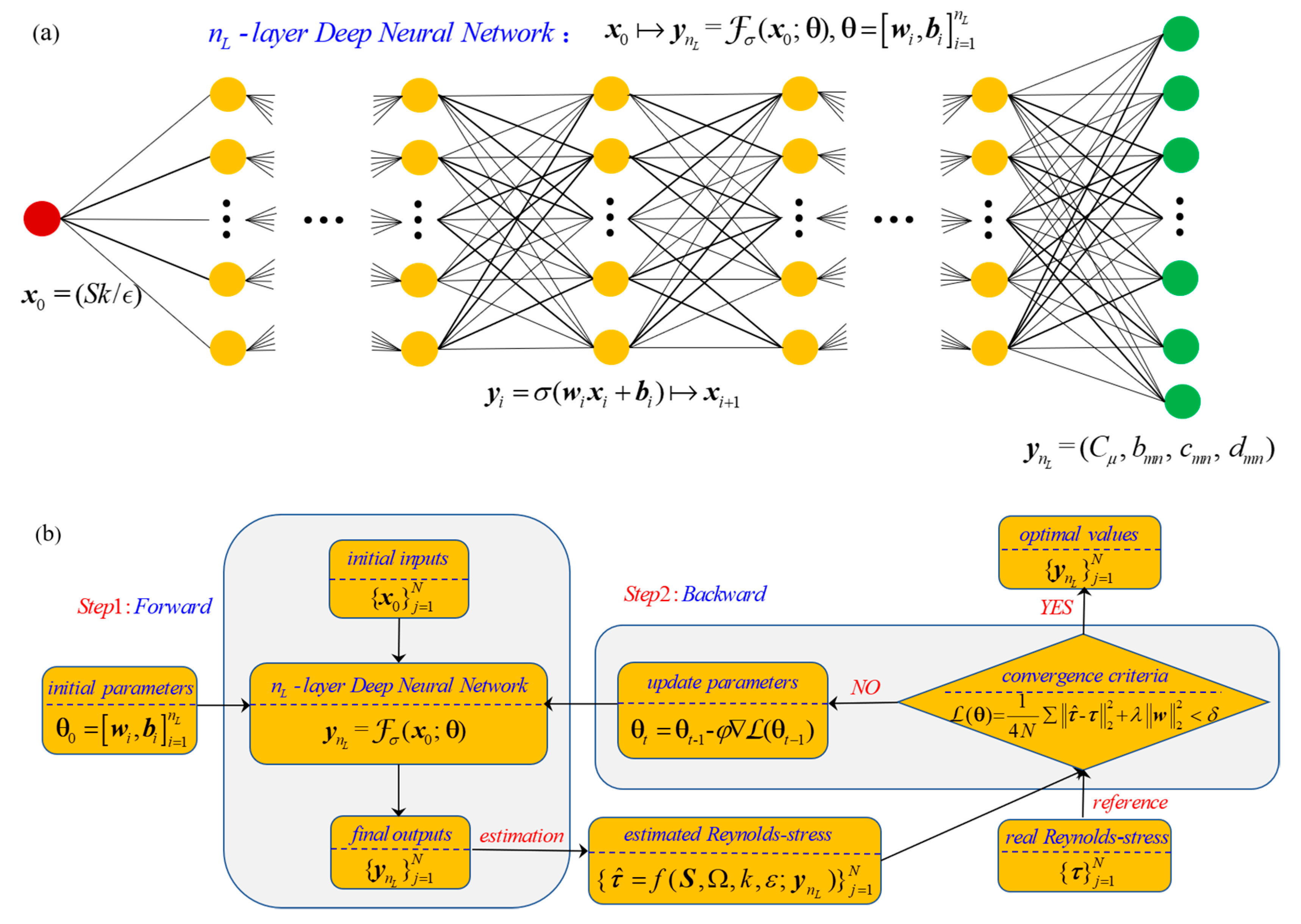
The fully-connected DNN architecture used herein is shown in Figure 2a, which is a cascade of several hidden layers of nonlinear processing units. The dimensional shear parameters $Sk/ϵ={\left(2S_{ik}{S}_{ik}\right)}^{1/2}k/ϵ$ as mean-flow invariants at various $R{e}_{\tau }$ are selected as initial inputs $x_0$ and the final outputs y_nL = (C_μ, b_mn, c_mn, d_mn) are the closure coefficients. Each successive layer uses the outputs from the previous layer as inputs, thus resulting in a hierarchical representation of learned features. Finally, a data-driven model is established to represent the mapping relationship between the closure coefficients and mean-flow quantities, viz,

$${\mathit{x}}_0\mapsto {\mathit{y}}_{n_L}={\mathrm{F}}_{\sigma }({\mathit{x}}_0;\mathsf{\theta }), \mathsf{\theta }={[{\mathit{w}}_i,{\mathit{b}}_i]}_{i=1}^{n_L},$$

(28)

where F_σ is the equivalent function representing the overall $n_L$-layer DNN-based data-driven model and $\mathsf{\theta }$ denotes all learned parameters, including the weights ${\mathit{w}}_i$ and the basis ${\mathit{b}}_i$ in each layer.

Figure 2b shows a complete optimization procedure to train this DNN-based data-driven model, which is controlled by the loss function:

$$L(\mathsf{\theta })=\frac{1}{4N}\mathsf{\Sigma }||\widehat{\mathit{\tau }}-\mathit{\tau }|{|}_2^2+\lambda ||\mathit{w}|{|}_2^2,$$

(29)

where $\mathit{\tau }$ and $\widehat{\mathit{\tau }}$ are the real stress vector and reconstructed stress vector according to Equation (25), respectively, and $\lambda$ is a regularization coefficient to prevent overfitting. N is the number of training samples. The rectified linear unit (ReLU) is used as the activator. The Adam (adaptive-moment-estimation) algorithm [51] is adopted to update parameters $\mathsf{\theta }$. Other hyper-parameters are set to $\lambda ={10}^{-3}$ and φ $=$10⁻⁵ (the step size). The number of hidden layers is set to 9, and the number of nonlinear units in each layer is 12, 18, 21, 27, 32, 35, 30, 28, and 27, respectively. After 5000 training epochs, iterative calculations are stopped when the tolerance error converges to $\delta =$10⁻⁴.

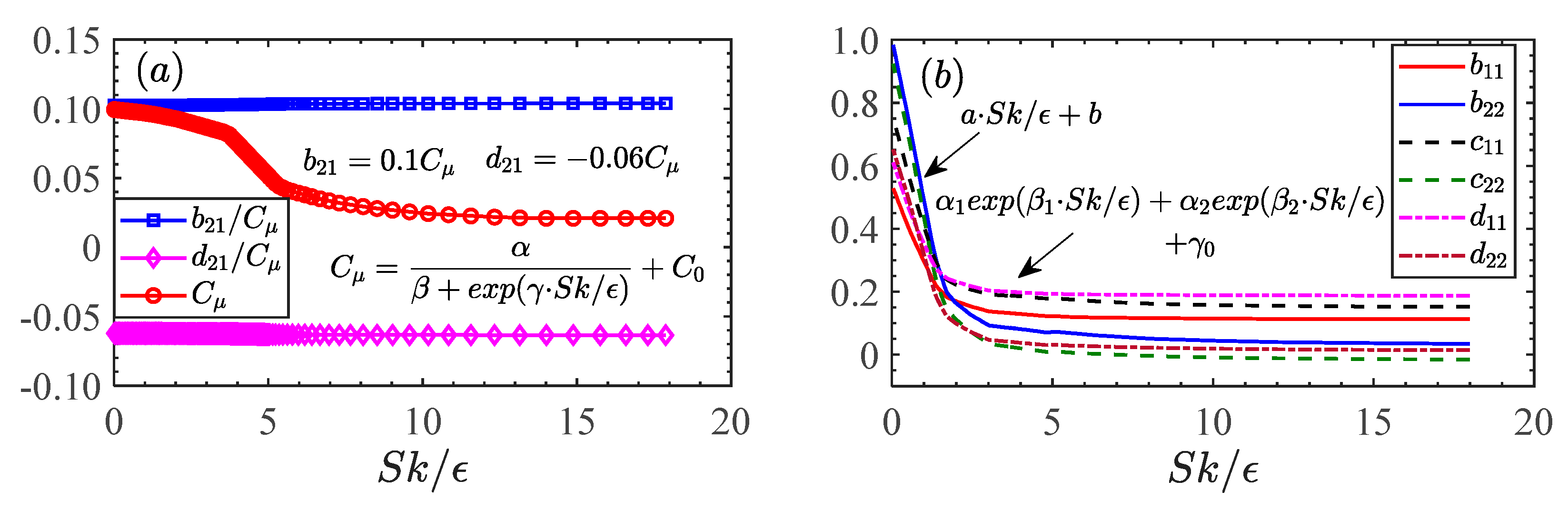
To improve the smoothness of input-output pairs, the explicit analytic forms of F_σ$:x_0\mapsto y_{n_L}$ is further given in Figure 3, which enhances the robustness of RANS-based numerical simulations. In traditional pointwise-based trainings (e.g., Wang et al. [43]), numerical convergence may be a problem due to the spatial non-smoothness of Reynolds stresses. In addition, the derivatives of Reynolds stresses are used in RANS equations, therefore, the smoothness is more important than the pointwise accuracy. The explicit re-parameterization adopted herein is very important otherwise alternative methods are taken to improve the smoothness.

To reduce the sensitivity to re-parameterization coefficients, we select proper function forms based on three rules below: (i) That Reynolds stresses can become infinite for any possible $Sk/ϵ$ should be avoided [52]. For example, a quadratic function is unsuitable for $C_{\mu }$. As an approximate alternative, the negative exponential function of $Sk/ϵ$ is selected. (ii) To avoid numerical instabilities due to the high sensitivity to strain-dependent coefficients, the nested transcendental functions should be averted [53]. For an exponential function, $e^a/e^{a+\delta }\approx 1$ for a limited small $\delta$. (iii) All coefficients should reduce to non-zero values at the high level of $Sk/ϵ$ to preclude numerical instability [53]. According to the rules above, we select the negative exponential function, of which the advantages have been confirmed by Weatheritt and Sandberg [54]. Finally, these coefficients in the Reynolds shear stress reads

$$C_{\mu }=\frac{\alpha }{\beta +\exp (\gamma Sk/ϵ)}+C_0, b_{21}=0.10C_{\mu }, d_{21}=-0.06C_{\mu },$$

(30)

where the values of $\alpha$, $\beta$, $\gamma$ and $C_0$ are 30.8, 250, 1.0, −0.03 and 0.22, 0, 0.41, 0.02 for $Sk/ϵ<5.0$ and $Sk/ϵ\ge 5.0$, respectively. The coefficients in the normal Reynolds stress obey

$${\xi }_{mn}=\{\begin{array}{cc}{\alpha }_1\exp ({\beta }_{1}Sk/ϵ)+{\alpha }_2\exp ({\beta }_{2}Sk/ϵ)+{\gamma }_0,\hfill & \hfill Sk/ϵ\ge 1.4\\ aSk/ϵ+b,\hfill & \hfill \mathrm{otherwise}\end{array}$$

(31)

where ${\xi }_{mn}$ stands for the learned closure coefficients $b_{11},b_{22},c_{11},c_{22},d_{11},d_{22}$ and the values of ${\alpha }_1$, ${\beta }_1$, ${\alpha }_2$, ${\beta }_2$, ${\gamma }_0$, $a$ and $b$ are shown in

Table 1. Values of ${\alpha }_1$, ${\beta }_1$, ${\alpha }_2$, ${\beta }_2$, ${\gamma }_0$, $a$, and $b$ as parameters appearing in closure coefficients.

	${\mathit{\alpha }}_1$	${\mathit{\beta }}_1$	${\mathit{\alpha }}_2$	${\mathit{\beta }}_2$	${\mathit{\gamma }}_0$	$\mathit{a}$	$\mathit{b}$
$b_{11}$	0.12	−0.51	0.87	−2.28	0.11	−0.24	0.53
$b_{22}$	0.10	−0.18	1.82	−1.71	0.03	−0.53	1.00
$c_{11}$	0.07	−0.17	1.11	−1.92	0.15	−0.36	0.75
$c_{22}$	1.30	−1.52	0.10	−0.30	0.02	−0.53	0.95
$d_{11}$	0.09	−0.57	0.46	−1.88	0.19	−0.26	0.61
$d_{22}$	0.93	−1.54	0.07	−0.29	0.01	−0.36	0.67

.

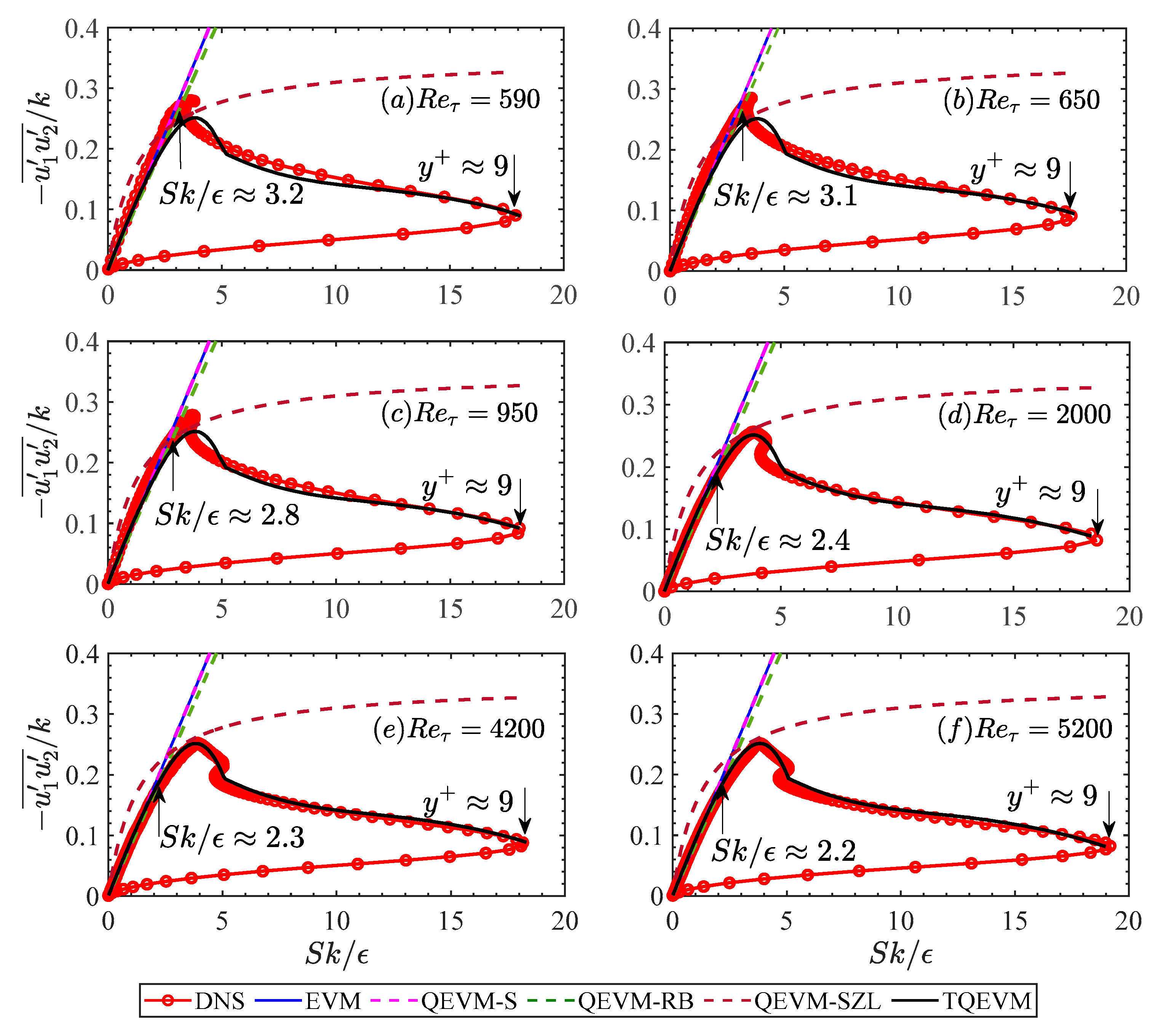
The learned $C_{\mu }$ agrees well with 0.09 in narrow regions far from the wall, which is the optimal value of $C_{\mu }$ in traditional QEVMs as well as the slope of shear stress-strain corresponding to the regions $Sk/ϵ\le 2.2~3.2$ in Figure 4. It can be, to some extent, used as an indicator of the success of the DNN-based regression model in Figure 2. Besides, Figure 3 shows that the closure coefficients related to shear stresses perform strong linear correlations (Figure 3a), and the closure coefficients related to normal stresses behavior in a very similar pattern (Figure 3b). The fact that linear coefficient $C_{\mu }$ reduces with increasing $Sk/ϵ$ (corresponding to the reduction of the wall distance) indicates an increase in the nonlinearity of shear stress when close to the wall.

4. Model Validation and Evaluation

4.1. Prior Validation and Comparisons

The performance of proposed TQEVM itself is validated using prior testing on datasets at $R{e}_{\tau }=$ (590, 650, 950, 2000, 4200, 5200). For comparisons, results of linear EVM (with the standard k-$ϵ$ model), previous QEVMs (QEVMs proposed by Speziale [34], Rubinstein and Barton [37], and Shih, Zhu and Lumley [38] are denoted as QEVM-S, QVEM-RB, QEVM-SZL, respectively) are also given.

4.1.1. Reynolds Stress

Figure 4 shows that Reynolds shear stress offered by all models except for QEVM-SZL falls almost exactly on the DNS results within the range of approximately $Sk/ϵ\le 2.2~3.2$. However, once $2.2~3.2<Sk/ϵ\le 18~19$, the Reynolds shear stress by EVM and QEVMs seriously deviates from DNS results, while TQEVM still shows good agreement.

EVM and previous QEVMs give the same prediction for the Reynolds shear stress as $-\overline{{u^{\prime }}_1{u^{\prime }}_2}/k=C_{\mu }\left(Sk/ϵ\right)$ where $C_{\mu }=0.09$ (except for QEVM-SZL). However, the TQEVM provides $-\overline{{u^{\prime }}_1{u^{\prime }}_2}/k=C_{\mu }\left(Sk/ϵ\right)+\left(b_{21}-d_{21}\right){\left(Sk/ϵ\right)}^2/4$, in which the nonlinear terms improve predictions in the near-wall region where nonlocal effects are significant due to spatial inhomogeneity. Figure 5 shows the dimensionless shear parameter $Sk/ϵ$, and dimensionless quadratic mean velocity gradient ${\partial }^2{\overline{u}}_1/\partial x_2^2$ as functions of dimensionless wall distance $y^{+}$. Within $Sk/ϵ\le 2.2~3.2$, which corresponds to a narrow region far from the wall, the variation of $\partial {\overline{u}}_1/\partial x_2$ (${\overline{u}}_1$ is the axial mean velocity and $x_2$ is the direction normal to the wall) is small, resulting in weak nonlocal effects. Therefore, the in-phase stress-strain relationships in EVM and QEVMS achieve good performance in this region. However, in the range of $2.2~3.2<Sk/ϵ\le 18~19$, which corresponds to a near-wall region, the dominant component $\partial {\overline{u}}_1/\partial x_2$ of the mean velocity gradients vary dramatically, resulting in the large stress-strain misalignment due to nonlocal effects induced by strong spatial variations in the mean shear. As a result, the nonlinear terms in TQEVM play a significant role and improve predictions of shear stress, by contrast, EVM and QEVMs fail.

The normal Reynolds stress determined by various turbulence models are shown in Figure 6, Figure 7 and Figure 8. TQEVM agrees well with DNS results in a large range of $y^{+}$. EVM always gives the same value of 2k/3 for the normal Reynolds stress components. However, the normal stresses are in reality anisotropic even very close to the centerline of the channel. Therefore, EVM always fails. QEVM-S and QEVM-SZL offer nearly identical results with EVM, while QEVM-RB provides a slight improvement. All QEVMs under-predict the axial component of the normal Reynolds stress and over-predict the other two components. When close to the wall, the difference between normal stresses increases rapidly and the predictions by QEVMs seriously deviate from DNS results. Therefore, previous QEVMs only achieve slightly better performance than linear EVM.

4.1.2. Stress-Strain Misalignment

Here we further evaluate the validity of turbulence models using modeled stress-strain misalignment. Analogous to the cosine of the angle between vectors, a new indicator ${\beta }_{RS}$ is introduced as a measure of the alignment trend between the Reynolds stress and mean strain tensors, viz,

$${\beta }_{RS}=\frac{R:S}{\Vert R\Vert \cdot \Vert S\Vert },$$

(32)

where $R^{\prime }$ and $S$ are the Reynold stress and mean strain tensors, respectively. For symmetric tensors, $R::S=R_{ij}{S}_{ij}$, $\Vert R\Vert =(R_{ij}{R}_{ij}{)}^{1/2}$ and $\Vert S\Vert =(S_{ij}{S}_{ij}{)}^{1/2}$. Therefore, ${\beta }_{RS}$ is a number between 0 and 1. ${\beta }_{RS}=$ 1 represents in-phase relationships between $R$ and $S$ (an alignment behavior), while ${\beta }_{RS}=$ 0 corresponds to a “perpendicular” state (maximum misalignment between $R$ and $S$). Accordingly, ${\beta }_{RS}$ can be used to characterize the validity of turbulence models. For example, EVM always returns modeled ${\beta }_{RS}=1$, therefore, EVM is valid only in the regions of a turbulent flow where the corresponding real values are β_RS = 1 When ${\beta }_{RS}$ is far from 1, the simple linear relationships between the stress and strain are no longer satisfied, thus nonlinear terms must be added to turbulence models to correct the predicted alignment trend.

Figure 9 shows alignment indicators ${\beta }_{RS}(y^{+}$) obtained from DNS result and predicted by previous QEVMs and TQEVM in channel flow at various $R{e}_{\tau }$. The stress-strain alignment gradually improves as $y^{+}$ increases, however, it suddenly becomes worse after $y^{+}$ reaches a very large value, which corresponds to the region very far from the wall (around the centerline of the channel). Also, the minimum phase lag (corresponding to the maximum value of ${\beta }_{RS}$) for Reynolds stress is no less than $\pi /4$, and the value gradually increases as the Reynolds number increases. Therefore, there is a clear stress-strain misalignment in a flow.

Previous QEVMs always provide in-phase relationships for the Reynolds shear stress as EVM (nonlinear terms in QEVMs have no effects on the shear stress) and a mild separation of the normal Reynolds stress. Consequently, these QEVMs cannot accurately predict ${\beta }_{RS}$. However, the results from TQEVM agree well with DNS, owing to nonlinear relationships both for the Reynolds shear stress and the normal Reynolds stress.

4.1.3. Realizability Constraints

Also, the realizability of turbulence models are examined using the barycentric map [55], which is a linear domain providing a non-distorted visual representation of anisotropy, as an advantage over commonly used anisotropy invariant map [56]. The eigen decomposition of the Reynolds stress tensor reads

$$\overline{u_i^{\prime }{u}_j^{\prime }}=2k(\frac{1}{3}{\delta }_{ij}+v_{ik}{\mathsf{\Lambda }}_{kl}{v}_{lj}),$$

(33)

where $v_{ik}$ are eigenvectors and ${\mathsf{\Lambda }}_{kl}=\mathrm{diag}({\lambda }_1,{\lambda }_2,{\lambda }_3)$ is the diagonal matrix of eigenvalues (${\lambda }_1\ge {\lambda }_2\ge {\lambda }_3$, ${\lambda }_1+{\lambda }_2+{\lambda }_3=0$). Here, turbulent kinetic energy, eigenvectors, and eigenvalues represent the magnitude, orientation, and shape of the Reynolds stress, respectively. In the anisotropy phase space of the barycentric map, any anisotropy state is located as a point such that the linear relationship holds: $\left(x,y)=C_{1C}\left(x_{1C},y_{1C}\right)+C_{2C}\left(x_{2C},y_{2C}\right)+C_{3C}(x_{3C},y_{3C}\right)$, where $\left(x_{1C},y_{1C}\right)$, $\left(x_{2C},y_{2C}\right)$, and $\left(x_{3C},y_{3C}\right)$ correspond respectively to one component (1C), two-component axisymmetric (2C-axis), and three-component isotropic (3C-iso) states. The corresponding weights $\left(C_{1C},C_{2C},C_{3C}\right)$ are entirely determined by the eigenvalues ${\lambda }_i$ as $C_{1C}={\lambda }_1-{\lambda }_2$, $C_{2C}=2({\lambda }_2-{\lambda }_3)$, and $C_{3C}=3{\lambda }_3+1$. Thus, the weights are used herein to characterize the degree of stress anisotropy and any realizable turbulence should satisfy $0\le C_{1C},C_{2C},C_{3C}\le 1$. Note that weights are very sensitive to a slight difference of Reynolds stress components, especially the values of $C_{2C}$ and $C_{3C}$ (amplitude modulation with a multiplier of 2 or 3).

In Figure 10, all the QEVMs except for the proposed TQEVM give unrealizable solutions for Reynolds stresses with $C_{2C}>1$ and $C_{3C}<0$ when close to the wall. Moreover, QEVMs fail in most regions with large discrepancies of $C_{1C}$ between prediction and truth, and they also provide a larger $C_{3C}$ in low Reynolds numbers and a larger $C_{2C}$ in high Reynolds numbers. When close to the channel centerline, all models return to a 3C-iso state with modeled $C_{3C}=1$ as the strain vanishing, which conflicts with a mild anisotropic state in reality. As a result, a corresponding sudden descent of stress-strain misalignment in Figure 9 arises. It is noted that this circumstance is encountered in all algebraic models (not limited to models mentioned here), but fortunately, the influence can be ignored because of extremely low anisotropic degree and only a small region existing (shown in Figure 6, Figure 7 and Figure 8).

Form the above discussion, it can be concluded that the proposed TQEVM has clear advantages over EVM and previous QEVMs. TQEVM offers a more approximate description both for stress-strain misalignment and stress anisotropy as well as extends the scope of the resolution.

4.2. A Posterior Numerical Simulation

Four cases of fully-developed channel flows are selected for numerical comparisons: Case I with $R{e}_{\tau }=650$ [46], Case II with $R{e}_{\tau }=$ 1000 [49], Case III with $R{e}_{\tau }=$ 5200 [50] and Case IV with $R{e}_{\tau }=$ 8000 [57]. Case I and III are investigated to show the Reynolds-number extrapolation for which DNS data are readily available to examine the prediction performance. Case IV is chosen to demonstrate the capability of the proposed TQEVM at higher Reynolds number where DNS is computationally expensive and high-fidelity data are extremely rare. Besides, $R{e}_{\tau }=$ 8000 is such a special case that the logarithmic region of the streamwise Reynolds stress exists and does not overlap with that of the axial mean velocity [57]. In the mean velocity profile, an incipient logarithmic region appears until $R{e}_{\tau }=$ 4000 and an unambiguous logarithmic region at $R{e}_{\tau }=$ 5200.

Two-dimensional RANS simulations with TQEVM are performed using structured meshes due to homogeneity in the spanwise direction. The incompressible flow solver simpleFOAM [58] based on OpenFOAM (an open-source package) is adopted. The height of the computation domain is 2h and the length is $8\pi h$ (h is the half-channel height). Figure 11 shows the predicted axial mean velocity profile, where all quantities are normalized by the half-channel height and axial mean velocity at the channel centerline. The mean velocity here is averaged over three locations randomly selected in the streamwise direction. The results show that the axial mean velocity predicted by TQEVM is basically consistent with DNS results.

Furthermore, skin friction coefficients predicted by TQEVM agree well with DNS as shown in

Table 2. Comparison of skin friction coefficients by TQEVM and DNS for four given cases.

	$\mathbf{Case} \mathbf{I}: \mathit{R}{\mathit{e}}_{\mathit{\tau }}=650$	$\mathbf{Case} \mathbf{II}: \mathit{R}{\mathit{e}}_{\mathit{\tau }}=1000$	$\mathbf{Case} \mathbf{III}: \mathit{R}{\mathit{e}}_{\mathit{\tau }}=5200$	$\mathbf{Case} \mathbf{IV}: \mathit{R}{\mathit{e}}_{\mathit{\tau }}=8000$
DNS	0.00612	0.00519	0.00351	0.00320
TQEVM	0.00556	0.00493	0.00329	0.00309

. Note that the skin friction coefficients at $R{e}_{\tau }=650$, 1000 and 5200 are from DNS of Schultz and Flack [59] and that of $R{e}_{\tau }=8000$ is estimated according to classical Prandtl’s smooth flow formula with a set of log-law coefficients suggested by Bernardini, Pirozzoli and Orlandi [49], viz,

$$\sqrt{\frac{2}{C_f}}=\frac{1}{\kappa }\ln (\frac{R{e}_b}{2}\sqrt{\frac{C_f}{2}})+C-\frac{1}{\kappa },$$

(34)

where $C_f = 2{\tau }_w/(\rho u_b^2)$, Re_b = Re_τ(2u_b/u_τ), $u_b={\int }_0^{2h}\overline{u}dy/(2h)$, $\kappa =0.386$ and $C=4.30$.

5. Conclusions

In the work, we present a machine learning strategy to assist the development of RANS closure modeling, aiming at reducing both structural (model-form) and parametric (model-parameter) inaccuracies. First, a novel algebraic Reynolds stress model named as TQEVM is developed, where nonlocal effects on the anisotropy evolution of Reynolds stresses are accounted for by nonlinear terms with corresponding coefficients, thus achieving a more appropriate description of Reynolds stresses. The proposed TQEVM also guarantees the symmetry and contraction requirements. Furthermore, a data-driven model by fusion of a fully-connected DNN architecture is designed to determine the coefficients of the proposed TQEVM. The well-trained data-driven model using high-fidelity DNS data at various Reynolds numbers successfully learned the underlying relationships between the closure coefficients and mean-flow quantities, resulting in spatial-dependent optimal values of these coefficients. The learned coefficient related to the linear terms $C_{\mu }$ agrees well with the real slope of shear stress-strain in regions close to the channel centerline. Thus, machine-learning-assisted regression analysis used herein offers a new route to reducing model-parameter inaccuracy, further advancing the performance of a given model.

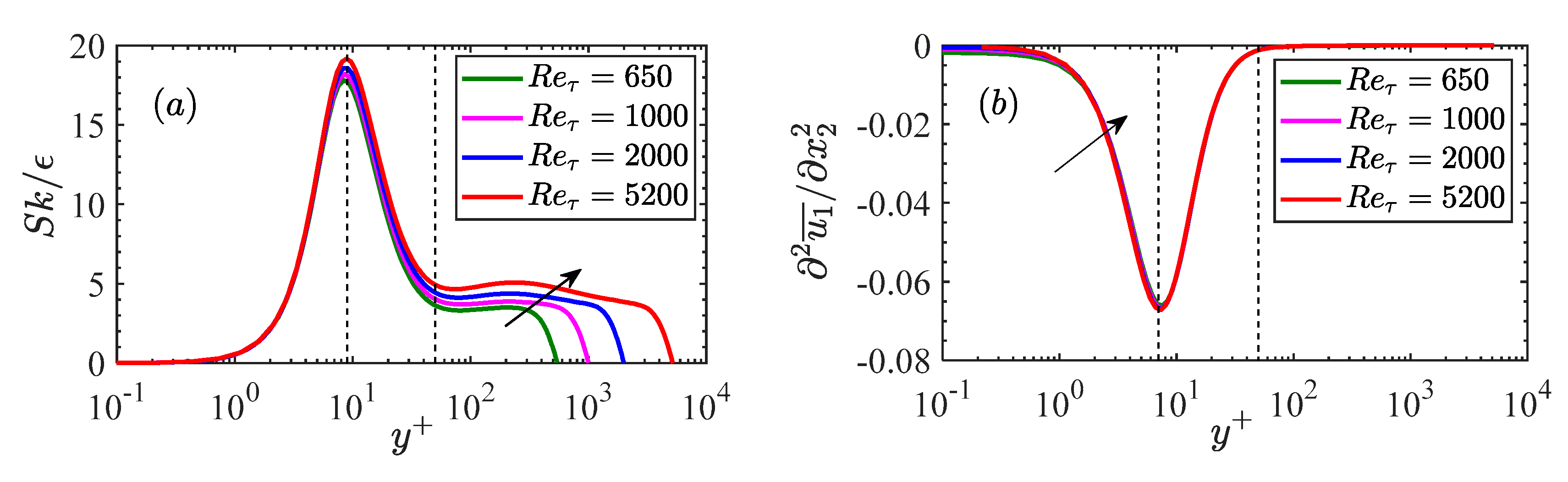
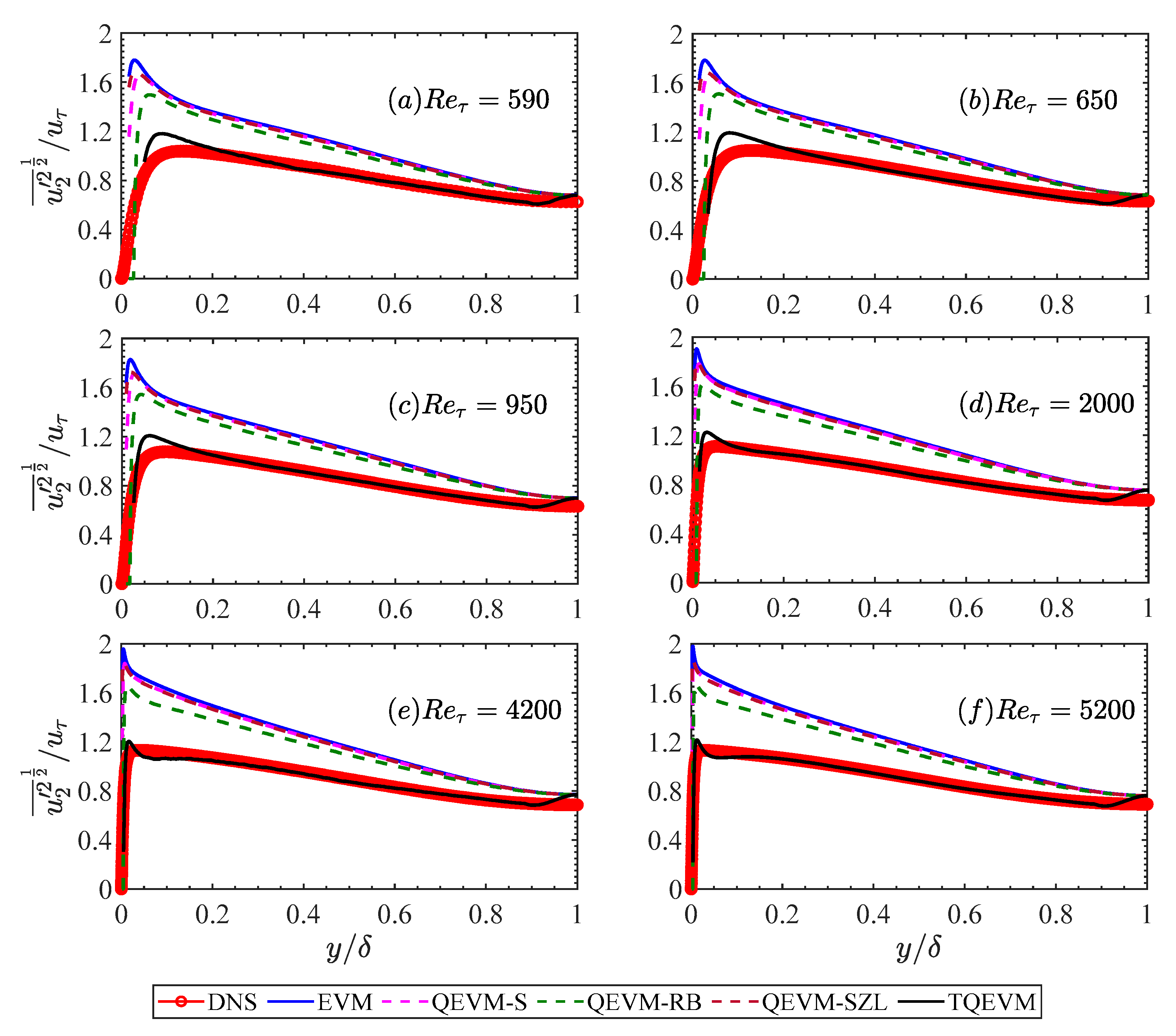
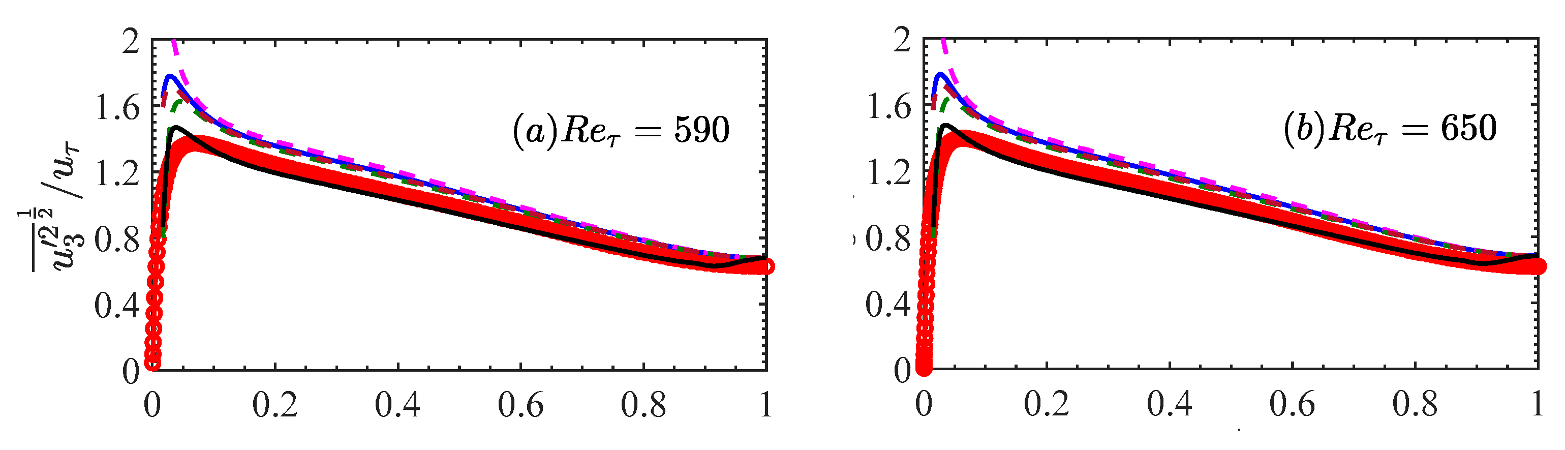
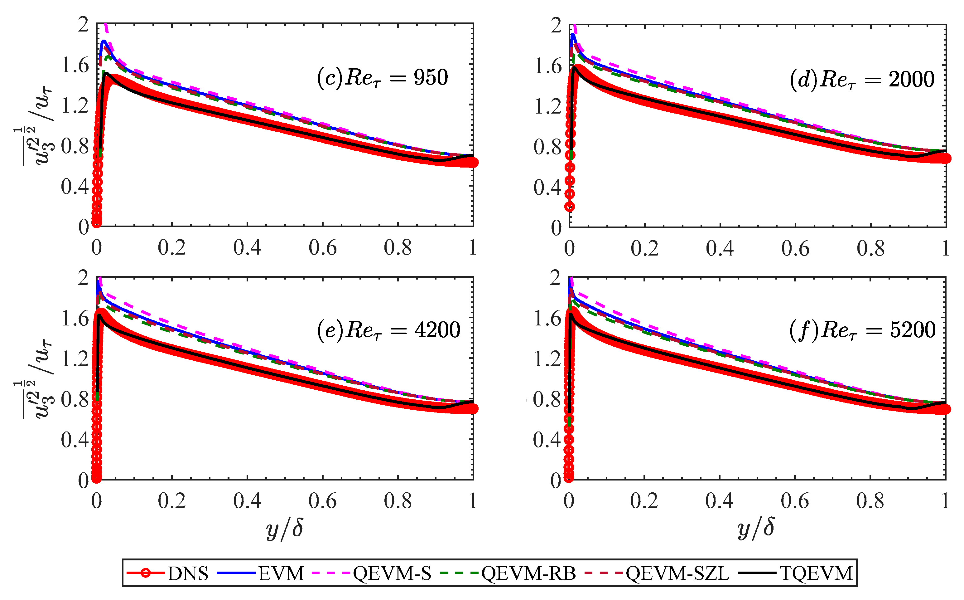
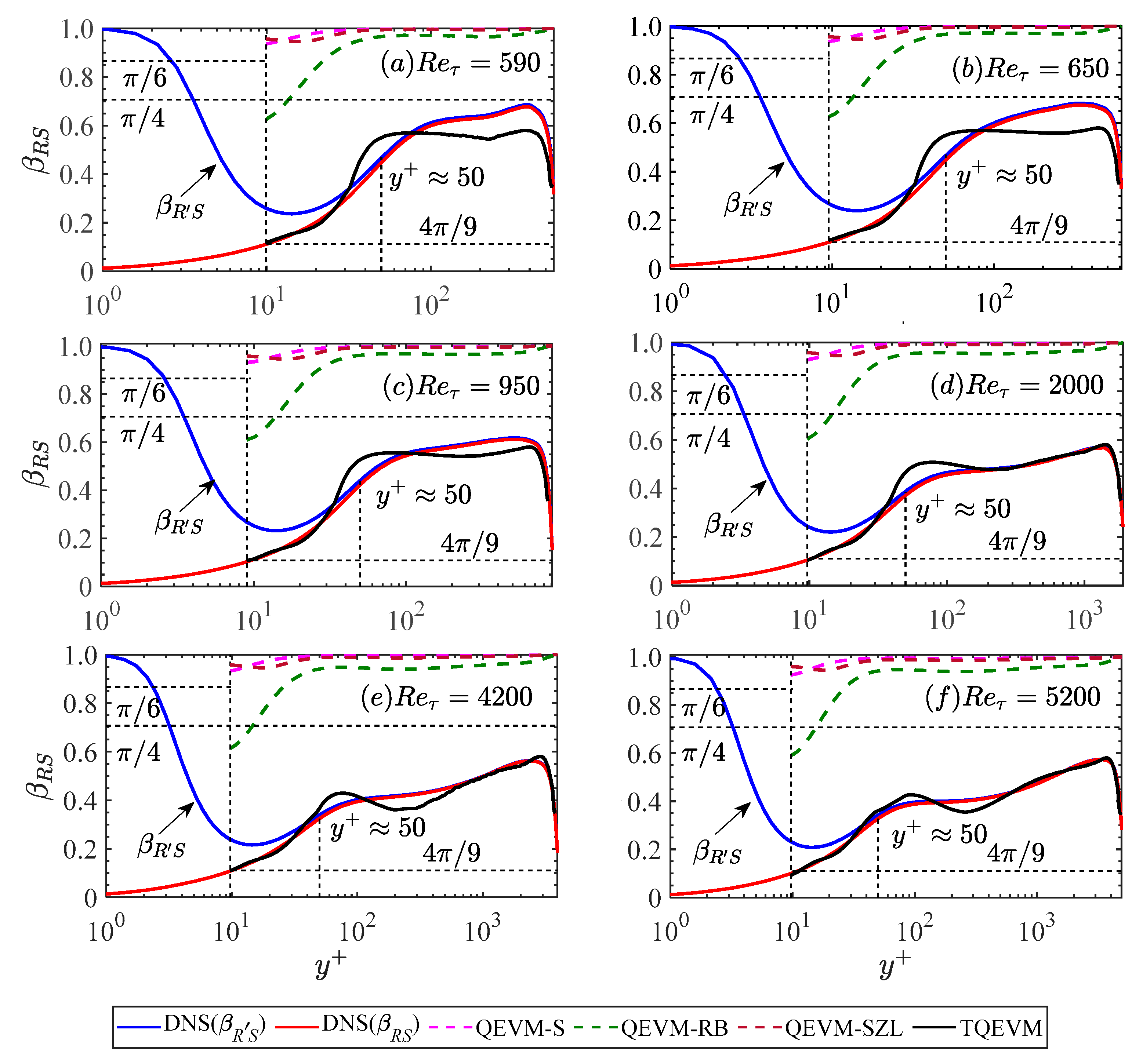
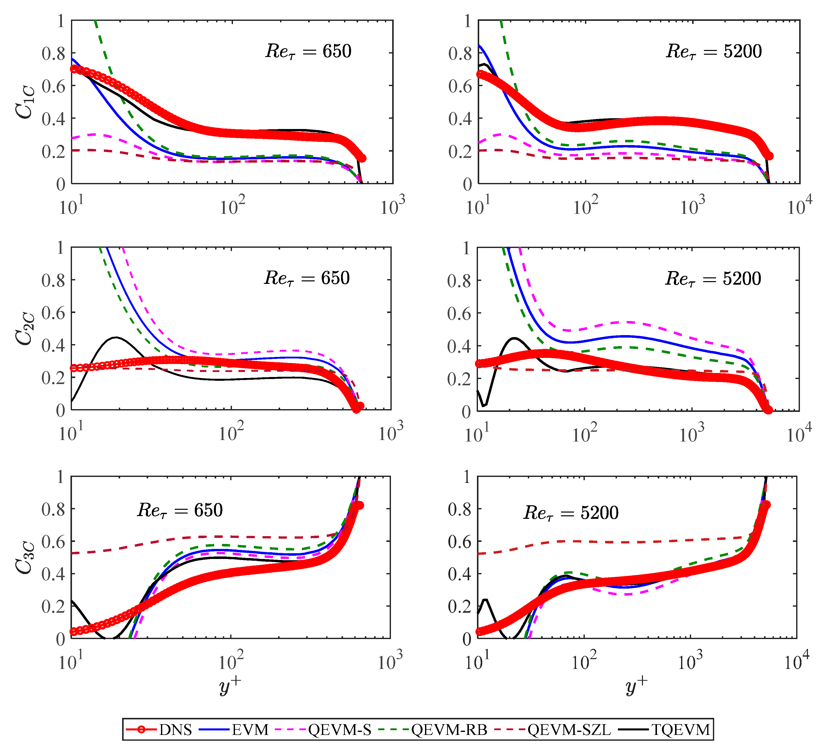
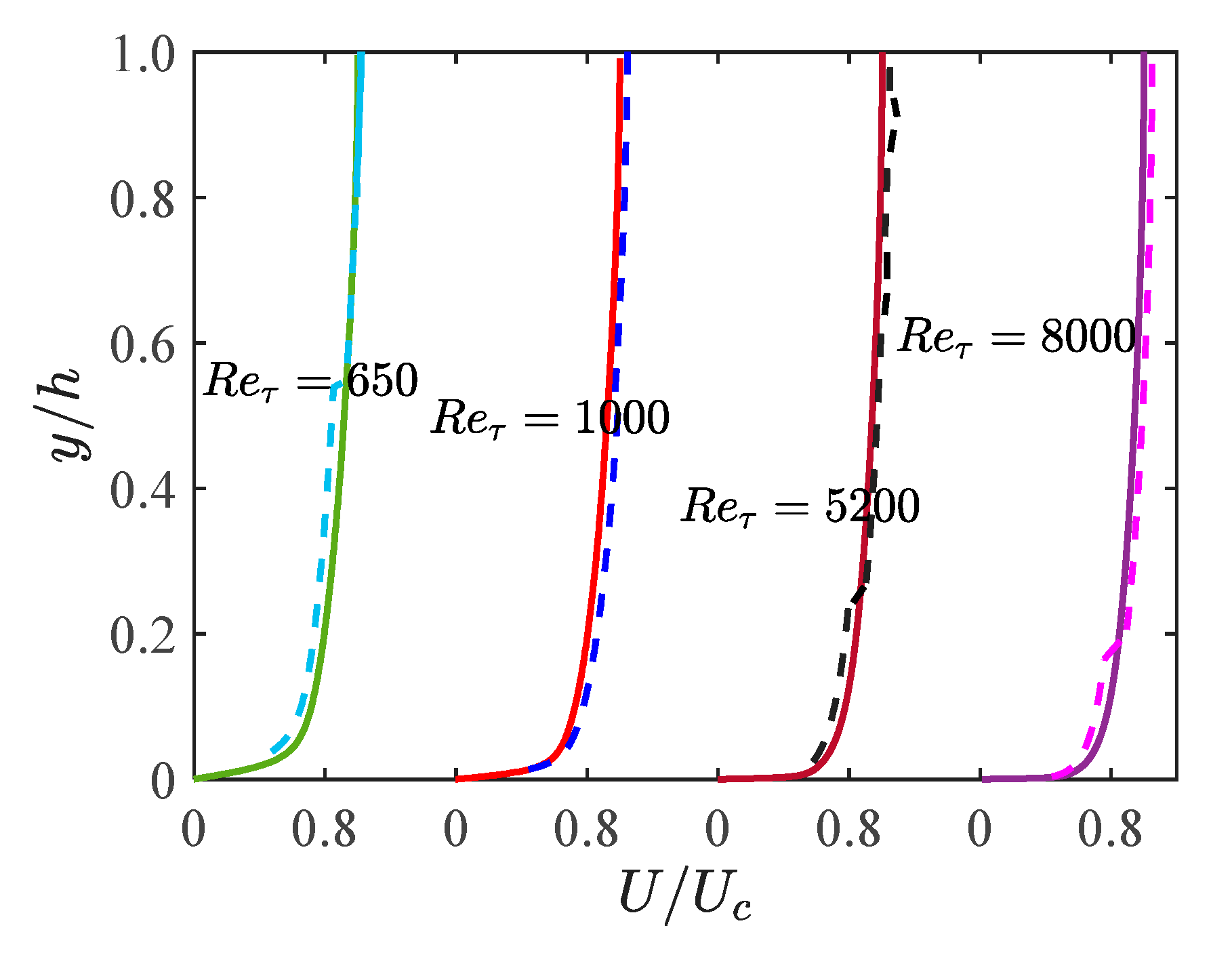
Finally, a complete validation including a prior and posterior testing is performed in detail to evaluate the performance of TQEVM. Comparative results show that the proposed TQEVM has clear advantages over traditional EVM and QEVMs in predictions both for the Reynolds shear stress and normal Reynolds stress by a wide margin. Besides, the proposed TQEVM extends the scope of resolution to $y^{+}\approx 9$ as well as provides a realizable solution. Nonlocal effects due to spatial inhomogeneity are significant in the near-wall region, resulting in a large stress-strain misalignment and strong stress anisotropy. Linear EVM and previous QEVMs misrepresent the real misalignment trend and under-predict the anisotropy magnitude. The failure is in large part due to insufficient consideration of nonlocal effects, which is a key source of error in previous RANS models. By contrast, the effects of nonlinear terms in the proposed TQEVM are dramatic, which contributes to improvements both for stress-strain misalignment and stress anisotropy. Accurate mean-flow quantities of interest are also obtained using numerical simulations with the proposed TQEVM.

It should be noted that TQEVM is expected to achieve improved predictions in other flows with strong spatial inhomogeneity, such as flows with secondary motion, three-dimensionality or curvature/rotation. TQEVM will be tested in these flows in the near future. Also, our model brings a new vision about how to select input features of a data-driven model for directly predicting Reynolds stresses: the second and higher-order derivatives of the mean velocity field should be introduced as supplements.