Article

Minimizing Power Consumption of an Experimental HVAC System Based on Parallel Grid Searching

1
College of Electrical Engineering and Automation, Shandong University of Science and Technology, Qingdao 266590, China
2
College of Engineering, Peking University, Beijing 100871, China
*
Author to whom correspondence should be addressed.
Energies 2020, 13(8), 2083; https://doi.org/10.3390/en13082083
Submission received: 19 February 2020 / Revised: 1 April 2020 / Accepted: 9 April 2020 / Published: 21 April 2020
(This article belongs to the Section G: Energy and Buildings)

Abstract

:
This paper proposes a parallel grid search algorithm to find an optimal operating point for minimizing the power consumption of an experimental heating, ventilating and air conditioning (HVAC) system. First, a multidimensional, nonlinear and non-convex optimization problem subject to constraints is formulated based on a semi-physical model of the experimental HVAC system. Second, the optimization problem is parallelized based on Graphics Processing Units to simultaneously compute optimization loss functions for different solutions in a searching grid, and to find the optimal solution as the one having the minimum loss function. The proposed algorithm has an advantage that the optimal solution is known with evidence as to the best one subject to current resolutions of the searching grid. Experimental studies are provided to support the proposed algorithm.

1. Introduction

Heating, ventilation, and air conditioning (HVAC) systems are usually comprised of the heating, air conditioning, and ventilation systems in residential or commercial buildings, to provide thermal comfort and air quality in indoor spaces [1,2]. The power consumption of HVAC systems is often more than half of total building power consumption [3]; however, many HVAC systems in practice have been running in a full load mode without considering the power consumption efficiency. Thus, it is important to find optimal operating points of HVAC systems in order to avoid unnecessary power consumption. The power consumption optimization is usually composed by two steps: (i) an analytical or numerical model is built to describe the relationship between the input and output variables of the HVAC system; (ii) an optimal operating point of the HVAC system is found to achieve the minimum power consumption subject to some constraints. The subject of this paper is on the second step.
Many optimization methods have been proposed to minimize the HVAC energy consumption in the literature, as summarized here in Table 1. Vakiloroaya et al. [4] reviewed different HVAC energy-saving strategies in the way of combining air conditioning technologies or changing the HVAC configurations. Lu et al. [5,6] presented a modified genetic algorithm (GA) for minimizing power consumption of HVAC systems, based on mathematical models of major components and their heat exchangers. Asiedu et al. [7], Chow et al. [8], Ullah et al. [9] and Kampelis et al. [10] also used the GA for the HVAC power optimization. Fong et al. [11] exploited the simulation tool TRNSYS [12] and TESS Libraries [13] to model the overall HVAC system for a local subway station, and took the robust evolutionary algorithm (REA) to optimize the energy consumption of the HVAC simulation models. Wemhoff et al. [14,15] proposed Lumped-HVAC (L-HVAC) method to build the HVAC model based on the coupled water balance and energy exchange calculations, and the Master Controller (MC) method to minimize energy for a system while meeting conditioning requirements. Zakula et al. [16] took the adaptive grid search technique to map the optimal heat pump performance as a function of the capacity, indoor and outdoor temperatures. Kim et al. [17] developed an energy performance prediction and optimization software to predict and optimize the energy consumption of a chiller system using a machine learning algorithm based on artificial neural network (ANN) models. Kusiak et al. [18] adopted the multi-layer perception (MLP) algorithm to construct energy consumption predictive models of an air handling unit, and the dynamic penalty-based electromagnetism-like algorithm (DPEM) to minimize the overall energy consumption. Wei et al. [19] constructed a quad-objective optimization problem to balance the energy consumption and the indoor air quality, and a modified particle swarm optimization algorithm (PSO) to minimize the total energy consumption of a dynamic overall HVAC systems. Kim et al. [20] developed an integrated meta-model for a lighting, heating, ventilating, and air conditioning system, and the GA algorithm for the minimum energy consumption with the constraints on both thermal and visual comfort. Aframa et al. [21] designed a supervisory model predictive controller (MPC) based on ANN models for minimizing the total cost of operating the HVAC system. Alibabaei et al. [22] discussed the development of three different strategic planning models including Smart Dual Fuel Switching System (SDFSS), Load Shifting (LSH), and LSH-SDFSS, and developed a novel smart dual fuel switching system for minimizing the energy cost of a residential HVAC system. Ghahramani et al. [23] introduced an adaptive hybrid algorithm to learn optimal HVAC settings with no prior historical data.
According to the above review of HVAC energy optimization strategies, there are two groups of optimization algorithms: the local optimization algorithm based on the gradient information and the global optimization algorithm based on heuristic searching techniques. The optimization problem for HVAC systems is in the multidimensional, nonlinear and non-convex nature. As a result, both algorithms have some limitations in finding a good solution. The former depends heavily on the given initial solution so that it is easy to yield a local optimum as the solution. The latter usually takes a high computational cost by using random initial solutions in many attempts; even so, it is not unclear whether the obtained optimal solution can be improved further.
This paper proposes a parallel grid search algorithm to find a global solution for the power consumption optimization problem of an experimental HVAC system. First, a multidimensional, nonlinear and non-convex optimization problem subject to constraint is formulated based on a semi-physical model of the experimental HVAC system. Second, the optimization problem is parallelized in order to simultaneously compute the optimization loss functions for different solutions in a searching grid, and to find the optimal solution as the one having the minimum loss function. The proposed algorithm is implemented in the Graphics Processing Unit (GPU), which has tens of thousands of computing cores for parallel computations. The main advantage of the proposed algorithm is that it does not suffer the above-mentioned limitations of the existing optimization algorithms. In particular, the proposed algorithm is exhaustive in terms of computing the loss function values of all feasible points in the searching grid, from which the optimal solution is obtained. Hence, it is confident that the obtained optimal solution is the best one subject to current resolutions of the searching grid.
The rest of the paper is organized as follows. Section 2 describes the problem to be solved. Section 3 presents the HVAC model and the proposed algorithm. Section 4 validates the proposed algorithm via experimental studies. Section 5 makes some concluding remarks.

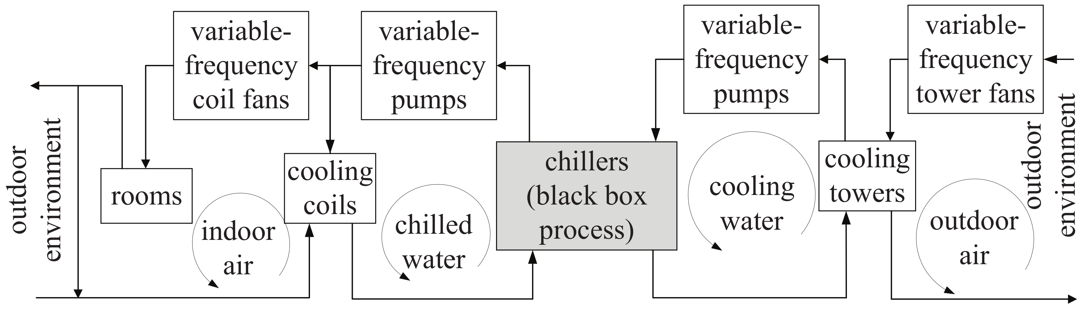
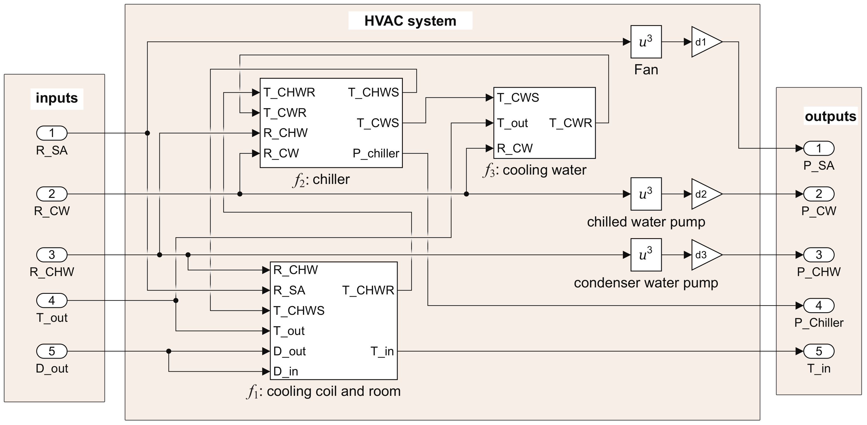
2. Problem Description

HVAC systems are usually composed by cooling coils, chillers, cooling towers, pumps, fans and rooms [1]; in terms of transferring energies, there are five loops being involved, namely, the indoor air loop, chilled water loop, refrigerant loop, cooling water loop and outdoor air loop as shown in Figure 1. For an experimental HVAC system in this paper, its input variables are the rotating speed R S A of a cooling coil fan, the rotating speed R C W of a cooling water pump, the rotating speed R C H W of a chilled water pump, the outdoor temperature T o u t and humidity D o u t , i.e.,
x : = R S A R C W R C H W T o u t D o u t T .
Here R S A , R C W and R C H W are controllable variables, while T o u t and D o u t are uncontrollable variables being determined by environmental conditions. The output variables are the power consumptions of the cooling coil fan, cooling water pump, chilled water pump and chiller, respectively denoted by P S A , P C W , P C H W and P C h i l l e r , as well as the indoor temperature T i n , i.e.,
y : = P S A P C W P C H W P c h i l l e r T i n T .
The objective is to minimize the total power consumption of the experimental HVAC system subject to some requirements on the comfortable temperature in rooms, by finding the optimal values of controllable variables in x . Thus, the optimization loss function is
P t o t a l = P c h i l l e r + P C H W + P C W + 2 P S A .
The last item on the right side of Equation (3) means that there are two cooling coil fans to respectively supply and return air in the HVAC system. Meanwhile, there is a constraint that the indoor temperature T i n is maintained in a required range, namely,
T i n , l b T i n T i n , u b ,
where T i n , l b and T i n , u b are the upper and lower bounds of T i n , respectively. Besides, it is assumed that the outdoor temperature T o u t and humidity D o u t are constant, because T o u t and D o u t are approximately unchanged during the time that T i n is changed by varying R S A , R C W and R C H W . In summary, the power consumption optimization problem for the HVAC system can be formulated as
R ^ C H W , R ^ C W , R ^ S A = arg min R C H W , R C W , R S A P t o t a l ,
subject to the constraint in (4).

3. The Proposed Algorithm

This section proposes a parallel grid search algorithm to find an optimal operating point for minimizing the power consumption of the experimental HVAC system.
First, a mathematical model of the experimental HVAC system is needed. The model is obtained by integrating the sub-models of major components of the experimental HVAC system in three parts: the cooling coil and room, the chiller and the cooling tower. Details in establishing the sub-models are irrelevant for the optimization problem and are reported elsewhere in our earlier work [24]. For the purpose of minimizing power consumption, the output variable vector y in (2) needs to be calculated for given values of the input variable vector x in (1). All major components of the experimental HVAC system are closely coupled via four intermediate variables z : = T C H W R T C H W S T C W S T C W S T . The HVAC model is
f x , y , z ; a , b , c , d = f 1 R C H W R S A T C H W S T o u t D o u t ; a T C H W R T i n f 2 T C H W R T C W R R C H W R C W ; w 1 , b 1 , w 2 , b 2 T C H W S T C W S P c h i l l e r f 3 T C W S R C W T o u t ; c T C W R f 4 R C W S R C W R S A ; d P C W S P C W P S A = 0 .
Equation (6) is schematically shown as an Matlab simulink diagram in Figure 2, where f 1 , f 2 and f 3 are represented by three square frames, and f 4 is decomposed as three subparts with the cubic function u 3 and model coefficients d 1 , d 2 and d 3 . The function f 1 is the model for the cooling coil and room,
f 1 = T o u t a 1 R S A R S A + a 4 1 e a 3 R S A 1 a 2 R S A R C H W 1 a 2 R S A R C H W e a 3 R S A 1 a 2 R S A R C H W T o u t T C H W S + a 5 R S A + a 4 a 6 T C H W S + a 7 R S A R C H W f H T o u t , D o u t f H T i n , D i n + a 8 ,
where a = [ a 1 , , a 8 ] T is the vector of model coefficients to be determined from experimental data. Since there is no humidifier, the indoor and outdoor humidities are assumed to be the same, i.e., D o u t = D i n . The function f H calculates the air enthalpy being associated with temperature T and humidity D [25],
H = f H T ; D = 1.01 T + 0.001 D 2005 + 1.84 T .
The function f 2 represents the chiller model being described by a two-layer feed-forward network as shown in Figure 3,
u = φ 1 w 1 x + b 1 , y = φ 2 w 2 u + b 2 .
Here x and y are the input and output of the system respectively; In this sub-model, the input variables are T C W S , R C W and T o u t , and the output variable is T C W R . Symbol u is the output of the hidden layer; w 1 and w 2 are the weight matrices of hidden and output layers respectively; b 1 and b 2 are their bias vectors; φ 1 · and φ 2 · are their activation functions, which are usually given as
φ 1 x = φ 1 , 1 x 1 φ 1 , n x n T , φ 1 , i x i = 1 e x i 1 + e x i , i = 1 , , n φ 2 = Identity Matrix .
Here n is the number of input variables of the chiller model. The function f 3 is the cooling tower model,
f 3 = 1 f H b T C W R f H T s ; D o u t + 2 c 2 R C W f K T C H W R T C W S T C W R + 4 f H b T C W R + T C W S T C W R + T C W S 2 2 f H T s ; D o u t + c 2 R C W f K T C H W R T C W S T C W R + 1 f H b T C W S f H T s ; D o u t c 1 f K T C W R R C W T C W R T C W S .
Here the function f H b calculates the enthalpy of saturated air and its wet bulb temperature T [25],
f H b ( T ) = α 0 + α 1 T + α 2 T 2 + α 3 T 3 .
The function f K is given by [25]
K = f K ( T C W R ) = 0.00175 T C W R + 1 .
c = [ c 1 , c 2 ] T is the vector of model coefficients. The function f 4 includes the models for the cooling and chilled water pumps as well as the cooling coil fan,
f 4 = d 1 R C H W 3 d 2 R C W 3 d 3 R S A 3 .
Here d = [ d 1 , d 2 , d 3 ] T is the vector of model coefficients. In this sub-model, the input variables are R C H W , R C W and R S A , and the output variable is P C H W , P C W and P S A .
Second, the main idea of the proposed algorithm is introduced [26]. In general, a grid search algorithm is an exhaustive searching algorithm, which can easily adapt to nonlinear, non-differentiable or even disconnected optimization problems. It selects a few values of each input variable, and formulates all possible combinations of the input variable values. The loss function of an optimization problem is calculated for all possible combinations to formulate a searching grid. The feasible solutions are found as the points in the searching grid satisfying the required constraints for the optimization problem. The optimal solution is the feasible point having the smallest loss function value. In the experimental HVAC system, the same type of rotating speed sensors are used to obtain the measurements of the three controllable variables R S A , R C W and R C H W ; in addition, the variational ranges of R S A , R C W and R C H W are normalized to be the same. Thus, it is reasonable to choose the same resolution r for the three variables. By separating the variational range with a uniform distance r, the number of different values for R S A is
N 1 = R S A , u R S A , l / r ,
where R S A , u and R S A , l indicate the upper and lower limits of the variational range of R S A . Similarly, the numbers of different values for R C W and R C H W are
N 2 = R C W , u R C W , l / r N 3 = R C H W , u R C H W , l / r .
The number of grid points to be searched is N 1 × N 2 × N 3 . The grid point is denoted by
x i , j , k = R S A , u R S A , l × i + i N 1 + N 1 + R S A , l R C W , u R C W , l × j j N 2 + N 2 + R C W , l R C H W , u R C H W , l × k k N 3 + N 3 + R C H W , l ,
where i, j and k with 1 i N 1 , 1 j N 2 and 1 k N 3 are the grid point indices. With the HVAC model in (6), values of y and z can be calculated for given values of the controllable variables R S A , R C W and R C H W in x i , j , k and the constant values of the uncontrollable variables T o u t and D o u t , based on the estimated coefficients a ^ , w ^ 1 , w ^ 2 , b ^ 1 , b ^ 2 , c ^ , and d ^ . The power consumption for each grid point is obtained as P i , j , k . After the power consumption is calculated for all grid points, the feasible grid points are determined as the ones satisfying the constraint in (4),
i I , j J , k K | T i n , l b T i n i , j , k T i n , u b ,
where T i n i , j , k is the indoor temperature associated with x i , j , k . The optimal solution is the feasible point with the smallest power consumption, i.e.,
x i 0 , j 0 , k 0 = arg min i I , j J , k K P i , j , k .
Third, owing to a fact that the calculations of P i , j , k for all grid points are independent of each other, the grid search algorithm is very suitable for parallel computations. Theoretically, if there are enough computing nodes, then these independent calculations can be performed simultaneously in a non-sequential manner, without communication among all the computing nodes. Thus, a parallel algorithm is designed by taking the advantage of a GPU’s Single-Instruction Multiple-Data (SIMD) property and a stream processing technique [27]. In the parallel algorithm, the calculation of P i , j , k is done by the GPU as a computation device. A Central Processing Unit (CPU) as the host is responsible for initializing the parameters of the HVAC model and managing the final result transmission with the GPU.
The general large-scale numerical computing technology developed on GPU by NVIDIA has shown evident advantages in floating-point operations and memory bandwidth [28]. With the potential of a GPU being exploited, one single computer has an entry-level super-computing power. The Compute Unified Device Architecture (CUDA) platform is a new software framework for the GPU parallel computing. It provides a programming model based on a three-level (Grid-Block-Thread) thread management structure as shown in Figure 4. In this model, the CPU serves as the host, which is responsible for logical transaction processing and serial computing, and the GPU serves as the device (or coprocessor) to execute instructions, which can be highly threaded in a so-call kernel function [28].
For the power consumption optimization of the HVAC system, the outdoor temperature T o u t and humidity D o u t are fixed and there are three optimization variables, namely, R S A , R C W and R C H W . It is known that each grid in the CUDA architecture has multiple two-dimensional blocks, and each block has multiple two-dimensional threads. Only three of these dimensions are required here. The grid point indices in (9) can be directly represented as
i = b l o c k . x , j = t h r e a d . x , k = t h r e a d . y ,
where b l o c k . x , t h r e a d . x and t h r e a d . y are the in-built variables in CUDA for the indices of thread and block, respectively. The algorithm starts with the formulation of the entire searching grid composed by N 1 × N 2 × N 3 points. Then, the global memory of GPU is allocated for the input and output variables, and the inputs of all the searching grids using (9) are transferred from the host memory to the global memory. Since the HVAC model coefficients, the outdoor temperature and humidity are commonly used in all threads, they are initialized in the common memory of GPU, which greatly improves the computing efficiency. Next, grid parameters ( b l o c k D i m and t h r e a d D i m in Algorithm 1) are set and the kernel function is launched. In the kernel function, after the computational tasks of all the threads are finished, the results are copied from the global memory back to the host memory. Finally, their power consumption values are compared to obtain the optimal grid point with the smallest power consumption.
Algorithm 1. Detailed algorithm for power consumption optimization.
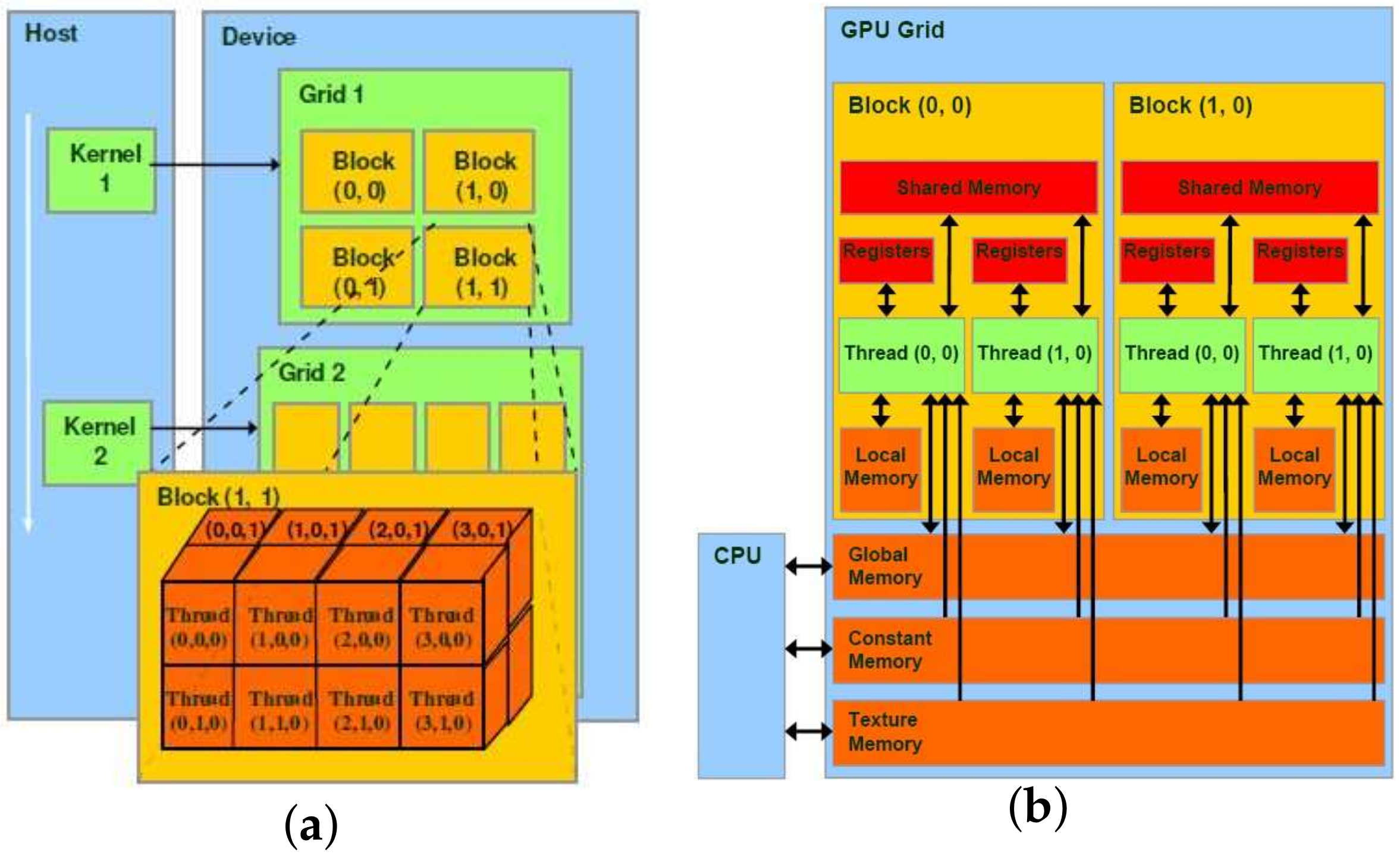
1. Divide the entire searching grid by N 1 × N 2 × N 3 and allocate the global memory
2. Formulate points of the searching grid for ( R S A , R C W , R C H W ) using (9)
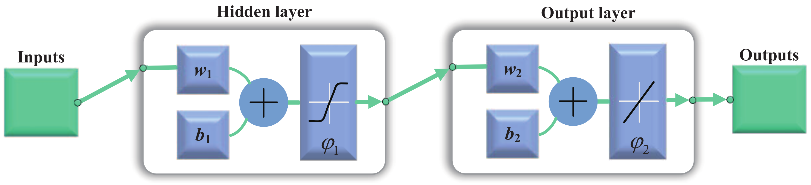
3. Initialize the HVAC model coefficients and T o u t and D o u t
4. Set the searching grid parameters and launch the kernels:
       o p t i m i z a t i o n K e r n e l < < < b l o c k D i m , t h r e a d D i m > > > (inputs, P t o t a l )
       _ _ shared _ _ EveryBlockPtotal threadDim ; i = block . x , j = thread . x , k = thread . y ; EveryBlockPtotal j , k is obtained from 3 by solving 6 for a given input i , j , k ; _ _ syncthreads ( ) ; P total i = min ( EveryBlockPtotal ) ;
5. Transfer all values of P t o t a l back to the host memory
6. Compare the values of P t o t a l to obtain the optimal solution x i 0 , j 0 , k 0 in (10)
Algorithm 1 gives the proposed algorithm in detail. The symbol o p t i m i z a t i o n K e r n e l stands for a kernel function, b l o c k D i m is the number of blocks and t h r e a d D i m is the number of threads per block. They are determined by the shared memory size configuration and registers per thread. Generally, t h r e a d D i m is usually a multiple of 64 [28]. It should be noted that their improper selection will lead to lower GPU occupancy. The symbol _ _ s h a r e d _ _ is a keyword to mean that this variable (EveryBlockPtotal) is a shared variable. All the threads in a block can share memories, synchronize and communicate by using shared variables. m i n ( · ) is a function to find the minimum of a data set. The symbol _ _ s y n c t h r e a d s ( ) guarantees that every thread in the block has completed instructions before the function m i n ( · ) is executed [27].

4. Experimental Studies

In this section, the HVAC model coefficients are estimated from experimental data, and the proposed algorithm is compared with the two other algorithms.

4.1. Model Coefficient Estimation

Real-time experiments are implemented in the experimental HVAC system, whose major components are shown in Figure 5. The experiments are implemented for 15 h, where the manipulated input variables are changed in turns from one constant value to another every 1000 s. It is observed that the HVAC system reaches a steady-state in the last 100 seconds of each 1000-s change. Thus, the data samples in the last 100 s of all 1000-s changes are extracted and merged together. Figure 6 and Figure 7 present the measured input and output variables, respectively. The sample period is 1 s. The HVAC model coefficients in (6) are estimated by minimizing the weighted summation of squared errors between measured and estimated outputs,
a ^ = [ 0.66338 0.73100 2.69039 × 10 6 0.37201 5.93943 1.70985 1.02587 22.41896 ] T .
w ^ 1 = 12.648 6.3743 0.2266 1.1952 1.4889 0.3175 0.3964 0.2549 2.631 3.5674 1.2782 5.7468 1.2873 3.6111 4.1862 0.8867 0.2039 1.5532 0.8243 0.2415 0.9726 1.2795 1.3493 0.6608 3.236 1.7607 3.2609 2.2888 , b ^ 1 = 1.578177 0.78776 3.870033 2.14653 0.16762 0.039405 2.94454 , w ^ 2 = 0.0811 2.2966 0.219 1.3604 2.5573 3.274 0.3694 0.0408 2.0244 0.0305 0.8858 2.8196 2.4118 0.2564 0.087 2.2905 0.0438 1.0062 3.0133 2.6992 0.3101 , b ^ 2 = 1.4322 1.2673 1.4859
c ^ = 9.325530 0.710525 T ,
and
[ d ^ 1 , d ^ 2 , d ^ 3 ] = 0.0079793 0.0067859 0.013137 T .
The measured and estimated outputs are compared in Figure 7. The corresponding coefficients of variation (CVs) are given Table 2 as a qualitative measure of model quality. The CV for a variable X and its estimate X ^ is defined as
c v , X = σ X X ^ μ X X ^ ,
where μ X X ^ and σ X X ^ are the sample mean and standard deviation of the error variable X X ^ , respectively. It can be seen that the estimated outputs are in line with the measured outputs, and the CVs are quite small.

4.2. Performance Comparison of Optimization Algorithms

This subsection compares the proposed algorithm with the interior-reflective Newton algorithm as a typical local optimization algorithm, and the genetic algorithm (GA) as a representative global optimization algorithm.
For the experimental HVAC system, the rotational speed of pumps and fans must be in a moderate range. In particular, the rotational speed of the chilled water pump should be larger than that of the cooling water pump. Thus, the value ranges of input variables R S A , R C W and R C H W are restricted to the interval in Equation (16),
20 % R S A 60 % 40 % R C W 80 % 10 % R C H W 60 % .
The rotational speeds are controlled by voltage signals in the experiment, so that the unit is the duty cycle with 0% and 100% for the minimum and maximum speeds respectively. A preliminary experiment is carried out to determine the feasible ranges of input variables in Equation (16) in order to meet with the required indoor temperature. The outdoor temperature is fixed to 30 C . For maintaining a desirable internal atmospheric environment, the indoor temperatures is constrained as
25 C T i n s i d e 27 C .
The hardware configuration for the optimization algorithms is shown in Table 3. Tesla K80 of NVIDIA with a total of 4992 cores is selected as the device to be used in the parallel grid search algorithm.
The results of the three algorithms are obtained as Table 4. First, for the interior-reflective Newton algorithm, the initial point must be given and it is generated by a random function within the interval in (16). It is concluded from Table 4 that different initial points lead to entirely different optimization results from the interior-reflective Newton algorithm. Second, the GA algorithm takes the default setup parameters in the MATLAB optimization toolbox, with the population size 100, the tolerance value 0.1, and a randomly-generated initial population. It is observed from Table 4 that the GA algorithm yields similar optimization results where values of P t o t a l are quite close in three trials. However, it is hard to know whether a smaller value of P t o t a l can be achieved by introducing more trials. Third, for the proposed algorithm, the numbers in (7) and (8) are selected as N 1 = N 2 = 40 40 0.1 0.1 = 400 , N 3 = 50 / 0.1 = 500 , because the resolution of the experimental devices for measuring rotational speeds is about 0.1. The optimal result is associated with P t o t a l = 2374.10 , which is much smaller than the counterparts from the interior-reflective Newton algorithm, and is slightly smaller than the best one.
P t o t a l = 2374.21 from the GA algorithm. Moreover, the propose algorithm is able to give the distribution of P t o t a l in Figure 8 for all points satisfying the indoor temperature constraint in (17). In order to observe the interior of Figure 8a, the 3D cloud image in Figure 8a is unfolded along the z axis ( R C H W ), and twenty 2D cloud images are obtained as shown in Figure 9. For the i-th sub-figure (i = 1,2,…, 20), the value of R C H W is given by R C H W ( i ) = 40 × i / 20 + 10 , while the horizontal and longitudinal coordinate variables are R S A and R C W respectively. The irregular shapes imply the presence of a non-convex optimization problem. The optimal point [33.0, 60.3, 14.2] in Table 4 is the darkest blue point (red asterisk) in the third column of the first row in Figure 9. It is worthy to note that there are several deep blue points in the cloud chart, such as the two black dots in Figure 9. The values of points nearby are listed in Table 5. Clearly, there are many locally optimal solutions, so that the optimization problem is clearly non-convex and nonlinear, which demonstrates the necessity of applying the proposed algorithm to solve the optimization problem. The proposed algorithm provides the entire solution space containing all values of the loss function corresponding to all operating points in the searching grid; thus, the best operating point is ready to be found. However, the GA algorithm only gives the solution path to the optimal operating point, which is difficult to be trusted without a comparison to other operating points in the entire solution space. Hence, unlike the GA algorithm, it is very confident that the proposed algorithm can find the best operating point for the given resolution of the searching grid.
Finally, the computation time is compared in Table 4. As expected, the interior-reflective Newton algorithm is the quickest, but its local optimal result is not acceptable. The proposed algorithm takes about the half computing time of the GA algorithm. As a comparison, the serial grid search algorithm takes 891,000 s (each grid search spends about 0.0139 s), which is more than 1300 times of the proposed algorithm. Thus, it is very necessary to do the grid search in a parallel manner. In summary, the proposed algorithm is able to guarantee a good optimization solution within an acceptable computing time.

4.3. Optimization Result Validation

This subsection provides experiments to validate the optimization results achieving the minimal power consumption.
Real-time experiments are implemented under the same experimental conditions as the ones for estimating HVAC model coefficients. Figure 10 shows the input variables in x of the experimental HVAC system. Multiple operating points are testified for the comparison purpose. The last constant parts of x in Figure 10 are associated with the optimal operating point from the proposed algorithm in Table 4. Measured output variables are compared with estimated counterparts from the HVAC model using model coefficients in (12)–(15). The consistency between the measured and estimated output variables in Figure 11 says that the estimated HVAC model is accurate. As expected, P t o t a l achieves the smallest value at the last part in Figure 11f. The actual value of P t o t a l is equal to 2509, with a small deviation ((2509–2374.1)/2374.1 % = 5.7 %) from the expected value 2374.10 in Table 4. This is due to a fact that the experimental conditions cannot be controlled the same as the assumed ones; in particular, the outdoor temperature T o u t fluctuates around 30 . Despite such a small deviation, the experiments clearly support the validity of the proposed algorithm in terms of finding an optimal operating point to achieve the minimal power consumption.

5. Conclusions

This paper presented a parallel grid search algorithm to find an operating point achieving the minimal power consumption for experimental HVAC systems. A multidimensional, nonlinear and non-convex optimization problem subject to constraints was formulated based on a mathematical model of the experimental HVAC system. By exploiting Graphics Processing Units, the optimization problem was parallelized to simultaneously compute optimization loss functions for different solutions in a searching grid. The proposed algorithm provided the entire solution space containing all values of the loss functions corresponding to all operating points in the searching grid. The optimal solution was obtained as the one having the minimum loss function and satisfying the required constraints. Thus, the main advantage of the proposed algorithm was that the obtained optimal solution was known with evidence to be the best one subjected to current resolutions of the searching grid. The proposed algorithm was validated in experimental studies and compared with two existing algorithms. In particular, the small deviation between the experimental and estimated results demonstrated that the proposed algorithm indeed found the optimal operating point to achieve the minimal power consumption.
As one future work, it is necessary to consider a non-constant outdoor temperature T o u t . The HVAC model in (6) has considered T o u t in the components f 1 and f 3 . The computational time of the proposed algorithm is about 11 minutes as given in Table 4. Hence, if T o u t is changing not too quickly, then it is ready to implement the proposed algorithm for different values of T o u t . The selection of sampling periods is another future work. A higher sample period reduces the computational time because fewer data samples are involved in optimization. However, it may deteriorate the optimization accuracy, because noises are omnipresent in the collected data samples, and the negative noise effects will be larger by exploiting fewer data samples in estimating the HVAC model parameters and calculating the optimal operating point.

Author Contributions

Conceptualization, J.W.; methodology, W.X.; software, W.X.; validation, J.W.; investigation, W.X.; data curation, W.X.; writing—original draft preparation, W.X.; writing—review and editing, J.W.; visualization, W.X.; supervision, J.W. All authors have read and agreed to the published version of the manuscript.

Funding

This research received no external funding.

Conflicts of Interest

The authors declare no conflict of interest.

Abbreviations

The following abbreviations are used in this manuscript:
R C H W chilled water pump speed
R C W cooling water pump speed
R S A cooling coil fan speed
T C H W S chilled water supply temperature
T C H W R chilled water return temperature
T C W S cooling water supply temperature
T C W R cooling water return temperature
T S A supplied air temperature through the cooling coil
T i n indoor temperature
T o u t outdoor temperature
D i n indoor humidity
D o u t outdoor humidity
P c h i l l e r power consumption of the chiller
P C H W power consumption of the chilled water pump
P C W power consumption of the cooling water pump
P S A power consumption of the cooling coil fan

References

  1. ASHRAE. HVAC Systems and Equipment; American Society of Heating, Refrigerating, and Air Conditioning Engineers: Atlanta, GA, USA, 2008. [Google Scholar]
  2. Real-Fernandez, A.; Navarro-Esbri, J.; Mota-Babiloni, A.; Barragan-Cervera, A.; Domenech, L.; Sanchez, F.; Aprea, C. Modeling of a PCM TES tank used as an alternative heat sink for a water chiller: Analysis of performance and energy savings. Energies 2019, 12, 3652. [Google Scholar] [CrossRef] [Green Version]
  3. Radzi, A.; Droege, P. Latest perspectives on global renewable energy policies. Curr. Sustain. Renew. Energy Rep. 2014, 1, 85–93. [Google Scholar] [CrossRef] [Green Version]
  4. Vakiloroaya, V.; Samali, B.; Fakhar, A.; Pishghadam, K. A review of different strategies for HVAC energy saving. Energy Convers. Manag. 2014, 77, 738–754. [Google Scholar] [CrossRef]
  5. Lu, L.; Cai, W.; Soh, Y.C.; Xie, L.; Li, S. HVAC system optimization–condenser water loop. Energy Convers. Manag. 2004, 45, 613–630. [Google Scholar] [CrossRef]
  6. Lu, L.; Cai, W.; Xie, L.; Li, S.; Soh, Y.C. HVAC system optimization—In-building section. Energy Build. 2005, 37, 11–12. [Google Scholar] [CrossRef]
  7. Asiedu, Y.; Besant, R.W.; Gu, P. HVAC duct system design using genetic algorithms. HVAC R Res. 2000, 6, 149–173. [Google Scholar] [CrossRef]
  8. Chow, T.T.; Zhang, G.Q.; Lin, Z.; Song, C.L. Global optimization of absorption chiller system by genetic algorithm and neural network. Energy Build. 2002, 34, 103–109. [Google Scholar] [CrossRef]
  9. Ullah, I.; Kim, D. An improved optimization function for maximizing user comfort with minimum energy consumption in smart homes. Energies 2017, 10, 1818. [Google Scholar] [CrossRef] [Green Version]
  10. Kampelis, N.; Sifakis, N.; Kolokotsa, D.; Gobakis, K.; Kalaitzakis, K.; Isidori, D.; Cristalli, C. HVAC optimization genetic algorithm for industrial near-zero-energy building demand response. Energies 2019, 12, 2177. [Google Scholar] [CrossRef] [Green Version]
  11. Fong, K.F.; Hanby, V.I.; Chow, T.T. System optimization for HVAC energy management using the robust evolutionary algorithm. Appl. Therm. Eng. 2009, 29, 2327–2334. [Google Scholar] [CrossRef]
  12. Klein, S.A.; Beckman, W.A.; Cooper, P.I. TRNSYS—A Transient System Simulation Program; Mathematical Reference; Solar Energy Laboratory, University of Wisconsin-Madison: Wisconsin, USA, 2004; Chapter 4; Volume 4, pp. 120–161. [Google Scholar]
  13. TESS Library Documentation. TESS Component Libraries v2.0 for TRNSYS v16.0 and TRNSYS Simulation Studio; Thermal Energy System Specialists: Wisconsin, MD, USA, 2004. [Google Scholar]
  14. Wemhoff, A.P.; Frank, M.V. Predictions of energy savings in HVAC systems by lumped models. Energy Build. 2010, 42, 1807–1814. [Google Scholar] [CrossRef]
  15. Wemhoff, A.P. Application of optimization techniques on lumped HVAC models for energy conservation. Energy Build. 2010, 42, 2445–2451. [Google Scholar] [CrossRef]
  16. Zakula, T.; Armstrong, P.; Norford, L. Optimal coordination of heat pump compressor and fan speeds and subcooling over a wide range of loads and conditions. HVAC R Res. 2012, 18, 1153–1167. [Google Scholar]
  17. Kim, J.H.; Seong, N.C.; Choi, W. Modeling and optimizing a chiller system using a machine learning algorithm. Energies 2019, 12, 2860. [Google Scholar] [CrossRef] [Green Version]
  18. Kusiak, A.; Zeng, Y.; Xu, G. Minimizing energy consumption of an air handling unit with a computational intelligence approach. Energy Build. 2013, 60, 355–363. [Google Scholar] [CrossRef]
  19. Wei, X.; Kusiak, A.; Li, M.; Tang, F.; Zeng, Y. Multi-objective optimization of the HVAC (heating, ventilation, and air conditioning) system performance. Energy 2015, 83, 294–306. [Google Scholar] [CrossRef]
  20. Kim, W.; Jeon, Y.; Kim, Y. Simulation-based optimization of an integrated daylighting and HVAC system using the design of experiments method. Appl. Energy 2016, 162, 666–674. [Google Scholar] [CrossRef]
  21. Afram, A.; Janabi-Sharifi, F.; Fung, A.S.; Raahemifar, K. Artificial neural network (ANN) based model predictive control (MPC) and optimization of HVAC systems: A state of the art review and case study of a residential HVAC system. Energy Build. 2017, 141, 96–113. [Google Scholar] [CrossRef]
  22. Alibabaei, N.; Fung, A.S.; Raahemifar, K.; Moghimi, A. Effects of intelligent strategy planning models on residential HVAC system energy demand and cost during the heating and cooling seasons. Appl. Energy 2017, 185, 29–43. [Google Scholar] [CrossRef]
  23. Ghahramani, A.; Karvigh, S.A.; Becerik-Gerber, B. HVAC system energy optimization using an adaptive hybrid metaheuristic. Energy Build. 2017, 152, 149–161. [Google Scholar] [CrossRef] [Green Version]
  24. Xiong, W.; Wang, J. Semi-physical modeling static behaviors of an experimental HVAC system. Control Eng. Pract. 2020, 96, 104312. [Google Scholar] [CrossRef]
  25. McQuiston, F.C.; Parker, J.D. Heating, Ventilating, and Air Conditioning: Analysis and Design; John Wiley and Sons: New York, NY, USA, 2005. [Google Scholar]
  26. Steven, M.; LaValle, M.; Branicky, S.; Lindemann, S.R. On the relationship between classical grid search and probabilistic roadmaps. Int. J. Robot. Res. 2004, 23, 673–692. [Google Scholar]
  27. Sanders, J.; Kandrot, E. Parallel Programming in CuDA C. In CUDA by Example: An Introduction to General-Purpose GPU Programming; Addison-Wesley Professional: Boston, MA, USA, 2010; pp. 37–57. [Google Scholar]
  28. Nvidia, C.U.D.A. Programming Model. In Programming Guide Version 8.0; Nvidia Corporation: Santa Clara, CA, USA, 2016; pp. 8–15. [Google Scholar]
Figure 1. The schematic diagram of an experimental HVAC system.
Energies 13 02083 g001
Figure 2. A schematic diagram of the HVAC model ( D i n is connected to D o u t since D i n = D o u t ).
Energies 13 02083 g002
Figure 3. A two-layer feed-forward network as the chiller model.
Energies 13 02083 g003
Figure 4. Compute Unified Device Architecture (CUDA) parallel computing: (a) its execution model. (b) memory hierarchy [28].
Energies 13 02083 g004
Figure 5. The major components of an experimental HVAC system: (a) the cooling coil and room, (b) the chiller and cooling tower.
Energies 13 02083 g005
Figure 6. The measured input variables for estimating model coefficients: (a) R S A , (b) R C W , (c) R C H W , (d) T o u t and (e) D o u t .
Energies 13 02083 g006
Figure 7. The measureds (blue dot) and estimated (red solid) output variables for coefficient estimation: (a) P S A , (b) P C W , (c) P C H W , (d) P c h i l l e r and (e) T i n .
Energies 13 02083 g007
Figure 8. Distributions of the total power consumption from two angles: (a) the distributions satisfying the constraint of indoor temperatures (b) all the distributions.
Energies 13 02083 g008
Figure 9. Distributions of the total power consumption for twenty values along z axis.
Energies 13 02083 g009
Figure 10. The measured input variables for validating optimization results: (a) R S A , (b) R C W , (c) R C H W , (d) T o u t and (e) D o u t .
Energies 13 02083 g010
Figure 11. The measured (blue dash) and estimated (red solid) output variables for validating optimization results: (a) P S A , (b) P C W , (c) P C H W , (d) P c h i l l e r and (e) T i n p, as well as the total power consumption (f) P t o t a l = P c h i l l e r + P C H W + P C W + 2 P S A .
Energies 13 02083 g011
Table 1. Summary of the methods of modeling the heating, ventilation and air conditioning (HVAC) system.
ReferencesSystem to Be OptimizedOptimization VariablesCost FunctionOptimization Algorithm
[5,6]Static overall HVAC systemNumber of operating chillers chilled
water pumps, cooling coils,
condenser water pumps and cooling
tower fans, temperatures of chilled
water supply and condenser water
supply, air flow rate of supply
air and cooling tower fun,
chilled and condenser water flow
rate of pumps
Total energy consumptionModified GA
[10]Dynamic overall HVAC systemhourly HVAC temperature set pointscost of energyGA
[11]Static overall HVAC systemSet point of chilled water
supply temperature of chiller and
supply air temperature of AHU
Monthly energy consumptionREA
[14,15]Static two-room systemFan rotation speed, actuating damper,
pump rotation speed, chiller work input
Energy consumptionMC
[16]Static heat pumpEvaporator and condenser airflow rate,
condenser area fraction devoted
to subcooling
Total power consumptionAdaptive grid search
[17]Static chillerchilled water flow rate
cooling water temperature
outside dry-bulb temperature
outside wet-bulb temperature
dew-point temperature
outside relative humidity
hour, type of day
total Power consumptionANN
[18]Dynamic AHUChilled water flow rate,
supply fan VFD speed,
chilled water coil valve position,
chilled water coil supply temperature
Total energy consumptionDPEM
[19]Dynamic overall HVAC systemSupply air temperature and
static pressure setpoint
Total energy consumptionModified PSO
[20]Dynamic overall HVAC systemVenetian blind slat angle,
AHU supply air setpoint temperature,
AHU operation status,
Relative water flow rate of FCU,
Outdoor-air mixing ratio
Total power consumptionGA
[21]Dynamic overall HVAC systemControl signal of AHU,
RFH, GSHP and RFH
Total cost of operating
the HVAC system
MPC
[22]House energy systemNot mention *HVAC system energy costSDFSS, LSH, LSH-SDFSS
[23]Overall HVAC systemNot mention *Energy consumptionAdaptive hybrid metaheuristic
* The authors did not mention the optimization variables of the established model.
Table 2. The coefficients of variation (CVs) of output variables.
Output
variables
P S A /kW P C W /kW P C H W /kW P c h i l l e r /kW T i n s i d e /K
Coefficient of
variations
2.91%1.95%0.59%0.84%0.075%
Table 3. Hardware specifications.
Component TypeComponent Performance
CPUIntel Xeon E5-4640 v4, 2.1 GHz, 12 cores
GPUTesla K80, 562 MHz, 4992 CUDA cores
CPU memory64 GB
GPU memory24 GB
GPU peak floating-point
performance with double precision
2.91 Teraflops *
GPU compilerNVCC 8.0 **
* Teraflops mean that the trillion ( 10 12 ) of floating point operations per second. ** nvcc is a compiler driver that simplifies the process of compiling C code.
Table 4. Comparison of optimization algorithms.
AlgorithmOptimization Result P t o t a l Computing Time/s
Interior-reflective Newton
initial point: [58.3 78.3 34.2]
                [52.0 45.7 31.1]
                [36.3 56.7 13.4]

[58.82, 78.28, 34.27]
[56.33, 51.80, 33.91]
[36.31, 56.62, 14.74]

2629.76
2988.22
2413.10

23.53
26.87
13.56
parallel GA
initial point: random
                  random
                  random

[33.13 60.12 14.14]
[30.91 62.58 16.35]
[31.79 61.76 15.59]

2374.21
2390.33
2387.21

1238.83
1159.34
1108.72
Parallel grid search [ 33.0 , 60.3 , 14.2 ] 2374.10685.71
Serial grid search ≈891000
Table 5. Points near the local and global optimal points.
Global MinimumLocal Minimum 1Local Minimum 2
center2374.102393.182406.30
Up2430.082444.282442.10
DownNaN *NaNNaN
right2406.572409.712424.8
LeftNaNNaNNaN
Forward2425.042425.332441.43
backwardNaNNaNNaN
* NaN means this point does not satisfy the indoor temperature constraint.

