Relative Free Energy Function and Structural Theory of Thermoeconomics

Abstract

This paper explores the advantages of using relative free energy instead of exergy to build a mathematical theory of thermodynamic costs to diagnose malfunctions in thermal systems. This theory is based on the definition of a linearized characteristic equation that represents the physical behavior of each component. The physical structure of the system described by its energy interrelationships is called “primal”, and its derivatives are the costs and consumptions. The obtained costing structure is the mathematical “dual” of its primal. The theory explains why the F and P cost assessment rules and any other suggestion may (or may not be) rational under a given disaggregation scheme. A result of the theory is a new thermodynamic function, called the relative free energy, and a new parameter called deterioration temperature due to a component’s deterioration cause, characterized by a h-s thermodynamic trajectory describing the effects on the exiting stream. The relative free energy function allows for an exact relationship between the amount of used resources and the increase in entropy generation caused by the deterioration path of the component. This function allows the obtaining of, for the first time, an appropriate characteristic equation for a turbine and a new definition of efficiency that does not depend on the environment temperature but on its deterioration temperature. Also, costing with relative free energy instead of exergy may open a new path for more precise and straightforward assessments of component deteriorations.

1. Introduction

The aim of this paper is challenging since it questions all the concepts that have been traditionally used in thermoeconomics, also called exergoeconomics by other authors [1]. There is a consensus among practitioners that exergy is the thermodynamic property that best distributes production costs among various streams, which then helps to establish the economic costs of the streams that interact in any energy system. However, the exergy calculation has the shortcoming that it depends on the reference environment employed, which in turn is an arbitrary selection of the user and not a physical behavior of the system under analysis. If this is so, the concept of exergy efficiency, although more precise than the first law efficiency, still depends on the reference environment. This obviously applies also to its inverse, the unit exergy consumption, which is the precursor of the Theory of the Exergy Cost [2,3]. Efficiency and costing are in effect, two sides of the same coin.

The Exergy Cost Theory (ECT) is simple to understand and easy to implement computationally, and as a result, its use has taken off since 1986 when it was first published. A year earlier, G. Tsatsaronis proposed to identify all the currents of an energy system in fuels and products and thereby generate the exergoeconomic costs. The ECT facilitated the task by proposing general Fuel-Product cost allocation rules that made the costing of energy systems a quasi-routine matter. But the problem of selecting a reference environment remains and there might a consensus regarding which is the most suitable. However, convergent opinions are not mathematical proofs. Moreover, the word thermoeconomics adds an enormous responsibility to the researcher, as implicitly makes a fundamental connection between thermodynamics and economics.

Historically many economists, especially the so-called ecological economists, have approached thermodynamics. The work of [4] extensively describes the early connections between economists and energeticists. Perhaps the most rigorous work was that from Georgescu-Roegen [5]. He already discarded energy as a numeraire, pointing to entropy instead. He even went beyond by formulating the fourth law of thermodynamics, as the impossibility of complete recycling of materials, drawing a parallel with the second law as the impossibility of complete recycling of thermal energy. From there on, ecological economists have tried to use entropy more as a metaphor than as a tool that quantifies decisions.

On the other hand, thermodynamicists, mainly engineers, developed the concept of exergy. It is not the aim of this paper to describe the history, see [6], but to outline the conceptual roots of thermoeconomics. Exergy measures the theoretical ability to do work, therefore exergy efficiency will more precisely measure the performance of a machine. Yet the inverse of the efficiency describes the amount of resources consumed to obtain a product. And this is actually the definition of the physical cost, which in turn stands on the threshold of the economics. This is so because if we value resources in monetary units and add other costs such as equipment depreciation, maintenance and other expenses, one obtains the monetary costs of production not only of the final products but of the intermediate products [1,7,8]. This opened the door to comparing the costs of irreversibilities against the costs of operation and maintenance, which in turn naturally lead to propose improvements in the design of industrial processes. This was a paramount technological breakthrough.

Arguably, practicality and not mathematical precision is what is sought in exergoeconomic cost analysis because the cost is measured in monetary units. That said, the fluctuation of money is alien to the process designer, since it depends on external conditions that the practitioner cannot control. Consequently, exergoeconomics is a useful tool in the design of industrial processes, but it does not strive for the same precision associated with physical sciences. Its results depend both on the variability of money and on the measurement of irreversibilities with respect to the chosen reference state.

The question is whether to go back to the concept of exergy cost, which only measures how the physical resources consumed by the production plant are distributed. In so doing, one, at least avoid currency fluctuations and focuses on the diagnosis of malfunctions that occur in all industrial processes [9]. This opened a new technological path because no energy system deteriorates for a single cause, but for several at the same time with different intensities and with chains of causation that induce new malfunctions and dysfunctions. Thermoeconomic diagnosis, using exergy costs, can be applied on-line and is very useful when analyzing very complex plants. The disaggregation of any industrial energy system into subsystems allows understanding the process of the formation of physical costs, predicts failures and may keep the plant in optimal operating conditions. Yet the costs of malfunctions are still dependent on the reference state of the plant, which can be taken as fixed, or variable depending on external environmental conditions.

In other words, exergy is useful as an industrial diagnosis tool, equipment malfunction is essentially due to deterioration of the equipment itself, not to the definition of the reference environment. In short, exergetic diagnosis is not a precise and objective physical theory, but a very useful and agreed by the practitioners’ tool. The question now is, is there an exergy-like type function that could provide diagnoses independent from the reference state? This would mean that environmental conditions would, for sure, influence the industrial system, not because of an arbitrary designer’s selection, but through the environment’s own natural interaction with the process.

If this were possible, we could give a rigorous answer not only to the thermodynamics of energy systems but to the economics itself, and all without leaving the Second Law. Linking the concept of cost with thermodynamics is to bridge the gap between Physics and Economics. It would be a crucial conceptual step forward sought by economists, something like the Holy Grail of economics. Indeed, while economists have come a long way in mathematical applications, they have never been able to link their laws to any physical law, except for metaphors and analogies. In this way, the conventional separation between hard and soft sciences would be closer to a scale of hardness than to the hard/soft dichotomy.

This paper expands upon an early keynote lecture at Nancy University [10], and its objective is to come closer to a solution to this problem and investigate the concept of relative free energy, already proposed by Valero et al., [11], but with important precursors such as Baehr [12] and Alefeld [13]. To maintain the completeness of the work, the Theory of Exergy Cost is briefly described first, followed by the Structural Theory, [14]. This leads to analyzing whether the decisions made by the process analyst are or not supported by mathematical logic. These decisions are mainly the cost allocation rules, the level of aggregation, the fuel/product/waste definitions, and of course the exergy function and the reference state. This will allow discerning mathematical reasons from reasonable assumptions and go forward to a new thermodynamic function: the relative free energy function.

2. The Exergy Cost Theory

The exergy cost (kWh), otherwise known as cumulative exergy consumption [15,16] or presently adopted as embodied exergy according to some authors, measures the amount of exergy necessary to manufacture a product when the boundaries of the production plant, disaggregation level, and exergy efficiency of each component have been defined [2,3]. Herein, the exergy cost of a stream with exergy $Ex$ is denoted with an asterisk, $E{x}^{*}$, and its unit exergy cost is expressed as follows: $k^{*}\equiv E{x}^{*}/Ex$.

The process of costs allocation in productive systems requires a set of rules [3,17]:

• Resources Rule: The exergy cost of the flows entering a thermal system should be provided as input data. In the absence of further information, it can be assumed as equal to their exergy.
• Cost Conservation Rule: For each and every system component, the exergy cost of output flows is equal to the exergy cost of the input flows.
• Unspent Fuel Rule: Also known as Rule F. The unit exergy cost of an unspent fuel at the output of a system component is the same as that of the input fuel.
• Co-products Rule: Also known as Rule P. All products of the same quality at the exit of a system component have the same unit exergy cost.

There are other costing rules, dealing with special cases, particularly the case of wastes, by-products, condenser outlets, etc., which are outside of this short description of the outlined theory [18].

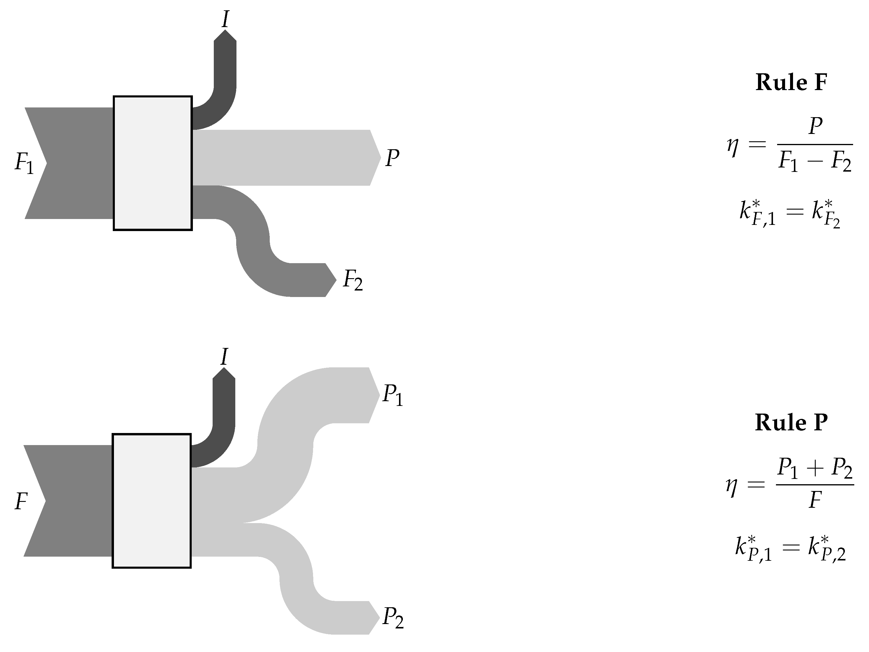
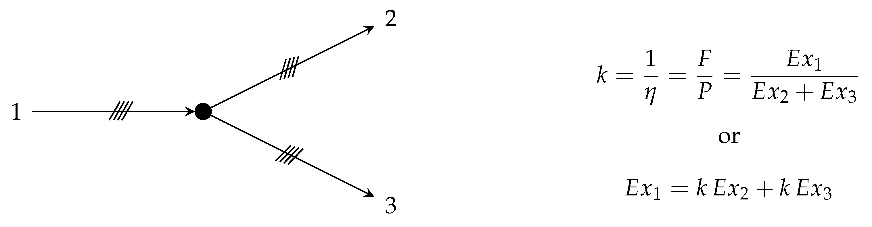
Summarizing, the (average) exergy cost is a conservative property and the production cost must be allocated to what one wants to produce. Therefore, when a process has multiple outputs, rules F and P need to be applied, see Figure 1, depending on the productive purpose of the processes.

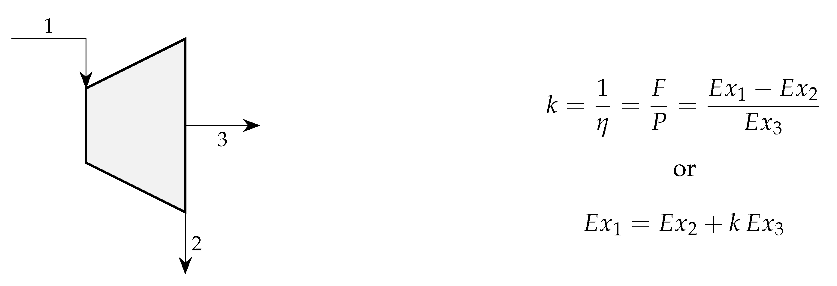
Let us see an example of application of these rules. Suppose first, a medium pressure steam turbine as shown in Figure 2, where the entering steam $F_1$ has 30 MW of exergy, it delivers a shaft work of $P=10$ MW and the exit steam $F_2$ still has 19 MW of exergy. Then, the exergy expended to produce P is $F_1-F_2=11$ MW, and its efficiency $\eta =P/(F_1-F_2)=0.909$.

If the turbine’s objective is to produce power, the full cost of that product should be charged to the shaft work. Accordingly, the rule F means that the unit exergy cost of the flowing steam remains unaltered. Suppose that the amount of exergy expended to produce the entering steam is 2.5 times greater than its exergy content, i.e., $k_1^{*}=2.5$ MW/MW. Then the rule F states that the unit exergy cost of the exit steam, $F_2$, is that of the entering steam, $F_1$, or $k_2^{*}=k_1^{*}=2.5$. Consequently, the amount of exergy needed to produce the shaft work will increase in $k_3^{*}=k_1^{*}/\eta =2.75$ MW/MW.

To explain Rule P, consider an electric generator added to a distributor as in Figure 3. It delivers two currents, 9 MW of net energy output and 0.5 MW for ancillary systems, at the expenditure of 10 MW of shaft work. Its efficiency becomes $\eta =(P_1+P_2)/F=0.95$. As both outlet streams are simultaneously required, the cost of its production must be allocated proportionally to both currents. Therefore, the Rule P states that the exergy cost per unit of exergy must be equal for the two currents. If the unit exergy cost of the shaft work was $k_1^{*}=2.75$ MW/MW, then the unit costs of the output electric streams become $k_2^{*}=k_3^{*}=k_1^{*}/\eta =2.895$ MW/MW. The reader may find many examples of application of these rules to a wide-ranging class of thermal systems in [19].

As it can be seen in this simple example, these rules link the concepts of the unit exergy cost, $k^{*}$, of the streams with the efficiency definition of the system’s components, $\eta =1/k$, one-to-one, where k is named the unit exergy consumption of the component. In other words, the cost of the final product increases as irreversibilities accumulate. If these increase, the efficiency of the components decreases and the costs increase accordingly. Thus, there is a direct connection between efficiency, cost, and irreversibility, when exergy is used as a measure of the energy flows of thermal systems. This is the essential message of the theory of exergy cost, which has been extensively used to assess the costs of many thermal systems.

However, a number of questions have arisen. First, based on its definition, the exergy cost depends on the plant disaggregation scheme. In other words, it cannot render a precise value because it depends on the analyst choice. For instance, a chemical plant produces ethylene and electricity, which are not produced in the same process but in the same plant; hence, either P or F rule could be applied. Therefore, the formation and type of the streams and how much and where the exergy has been consumed in the process must be analyzed. This detailed analysis provides a productive structure to which the rules can be applied in practical terms. A more detailed definition is more precise; however, there is the risk of not having measured data that corroborate the sensitivity of the obtained costs to variations in these data. There can be major discrepancies among practitioners regarding the definition of productive structures and the disaggregation method of the processes.

Second, the definition of exergy efficiency also depends on the analyst. For example, in a counter current heat exchanger, a stream becomes cooled, and another becomes heated. Hence, it heats, cools, or both, then, which stream assumes the production cost? Furthermore, not all components aim to save exergy (productive components). Certain other components in a plant are responsible for mitigating (the exergy of) wastes. Hence, it must be determined how to allocate costs to the components that process residues. Third, exergy and its related cost depend on the chosen reference environment. However, the physical behavior of the plant does not depend on the analyst choice. Additionally, the right choice of the energy-like function for describing the plant might be in doubt: energy, exergy, (Gibbs) free energy, or any other generic function.

Moreover, are the obtained costs average costs or marginal costs? The exergy of a stream measures its potential work with respect to a given environment, and the exergy cost measures how many irreversibilities have occurred in the manufacture of a stream or product plus its remaining exergy. The exergy cost can be considered an “exergy backpack” or “exergy footprint” of a stream or product, i.e., the past exergy synopsis (history) of the stream, whereas its exergy is the future energy potential of such a stream or its remaining capacity to produce work. Finally, can the exergy costs predict future degradations or describe only past irreversibilities?

Despite these doubts, the analyst aims to obtain reasonable costs. Thus, it is necessary to disaggregate the system as far as common sense advises. However, if costs depend on the disaggregation scheme what scheme is reasonable? Second, the definition of efficiency for each component requires caution. Is it possible to find a more rational definition of efficiency? Third, choosing exergy is apparently better than other energy-like functions because it provides a proxy for the locally usable energy. Are there better energy-like functions that predict the behavior of components? Fourth, the selected reference level for exergy must be realistic. Is it possible to avoid the dependence of costs from the chosen reference environment? Finally, the average costs should be useful in predicting how many additional resources compensate for the small system perturbations. Is there a theory capable of predicting exactly small system perturbations? While the current theory does not support these prudent conventions, practice does.

3. On the Linearity of Cost: The Structural Theory of Thermoeconomics

Any energy system that consumes resources and manufactures products can be characterized by a thermodynamic function E of the generic type, $E=m(h-T_{x}s)$ where m is the mass, h the enthalpy, s the entropy with respect to a certain reference, and $T_x$ the temperature to choose under certain conditions. When $T_x$ is zero, the function E is the enthalpy; when $T_x$ is the ambient temperature, E is the exergy; if $T_x$ is the temperature of the system, E is the Gibbs free energy function.

The mathematical behavior of any component u can be described through functions of the type:

$$E_i=g_i\left(\left\{x\right\},\left\{E_j\right\}\right)i\in {\mathcal{E}}_u$$

(1)

where $i\in {\mathcal{E}}_u$ are the input flows of component u and $j\in {\mathcal{S}}_u$ the output flows of component u, and $\left\{x\right\}$ is the set of its internal governing parameters, for instance, internal efficiencies, pressure relationships, temperature increases, geometric parameters, structural parameters, fluid dynamic parameters or heat transfer parameters. If the system environment is considered as the component “0”, then ${\mathcal{E}}_0$ is the set of the system outputs, and ${\mathcal{S}}_0$ is the set of input resources to the system.

Function Equation (1) does generally not relate inputs and outputs linearly. Because the only degree of freedom is the choice of $T_x$ (i.e., the choice of energy, exergy, Gibbs function, or any other function), it is likely that the complexity of the equation cannot be reduced to a linear relationship. However, such a continuous function allows for a Taylor series approximation. In addition, by choosing sufficiently small linear intervals, second-order terms can be discarded. The smaller the interval, the closer is the proposed behavior to reality. By applying this step, the following is obtained:

$$E_i=\{\begin{array}{cc}{\displaystyle \sum _{j\in {\mathcal{S}}_u}}{k}_{ij}\left(x\right)E_j\hfill & i\in {\mathcal{E}}_u\hfill \\ {\omega }_i(const.)\hfill & i\in {\mathcal{E}}_0\hfill \end{array}$$

(2)

which relates the inputs and outputs linearly through parameters $k_{ij}$, which substitute the internal parameters for each identified component. Furthermore, the coefficients $k_{ij}$ take the name of technical production coefficients in the input–output theory [20]. They are the (average) unit consumption of resource i necessary to produce stream j.

Owing to the linearity, the coefficients $k_{ij}$ coincide with derivatives (ceteris paribus) of the following type:

$$k_{ij}\equiv {\displaystyle \frac{\partial E_i}{\partial E_j}}$$

(3)

the advantage of a linear analysis is that it enables the understanding of many underlying assumptions in any cost allocation theory:

$$E_i=\sum _{j\in {\mathcal{S}}_u}\left({\displaystyle \frac{\partial E_i}{\partial E_j}}\right)E_{j}i\in {\mathcal{E}}_u$$

(4)

herein, this expression is called the component’s characteristic equation.

On the other hand, the globally considered plant will receive some resources, be these $E_0$, defined as:

$$E_0=\sum _{j\in {\mathcal{S}}_0}{E}_j$$

(5)

where ${\mathcal{S}}_0$ is the set of flows entering the plant (or leaving the environment).

The cost allocation is a basic application of the chain rule for derivative calculation, which is independent on the characteristic equations are linear or not, then the following expression for each flow of the system is satisfied:

$$\left({\displaystyle \frac{\partial E_0}{\partial E_j}}\right)=\sum _{i\in {\mathcal{E}}_u}\left({\displaystyle \frac{\partial E_0}{\partial E_i}}\right)\left({\displaystyle \frac{\partial E_i}{\partial E_j}}\right)$$

(6)

If we identify the marginal unit cost with the derivative:

$$k_i^{*}\equiv \left({\displaystyle \frac{\partial E_0}{\partial E_i}}\right)$$

(7)

the marginal unit cost of flows, could be determined by means of Equation (6), as follows:

$$k_j^{*}=\{\begin{array}{cc}{\displaystyle \sum _{i\in {\mathcal{E}}_u}}{k}_i^{*}{k}_{ij}\hfill & j\in {\mathcal{S}}_u\hfill \\ 1\hfill & i\in {\mathcal{S}}_0\hfill \end{array}$$

(8)

in other words, the unit cost of process u outputs are linearly related with the unit cost of input streams by means of the technical coefficients. In case of the system’s inputs, the marginal costs are known or made equal to one, which correspond to the external resources rule in the exergy cost theory.

The application of this equation explains the previously mentioned Rules F and P as a particular case. For example, a turbine (Figure 2) with the following defined efficiency is considered:

Suppose now, it is assumed that the characteristic equation of the turbine coincides with the exergy definition of the turbine. In the simulations of the turbine for a reasonably small working interval, k can be considered constant. By applying the unit cost Equation (8), the costs of outputs #2 and #3 are obtained:

$$k_3^{*}=k{k}_1^{*}\mathrm{and}{k}_2^{*}=k_1^{*}$$

(9)

hence, the result is Rule F, i.e., if a resource has not been totally consumed (stream 2), its unit cost is equal to that of the input resource (stream 1).

However, if a typical electric power distribution system is considered, see Figure 3 its efficiency can be expressed as follows:

Again, it is assumed that the characteristic equation of the distribution system coincides with its exergy definition. If k is constant, applying the unit cost Equation (2) results in:

$$k_2^{*}=k{k}_1^{*}\mathrm{and}{k}_3^{*}=k{k}_1^{*}$$

(10)

which explains why Rule P applies; that is, the unit costs of the products of the same nature produced in the same process are equal.

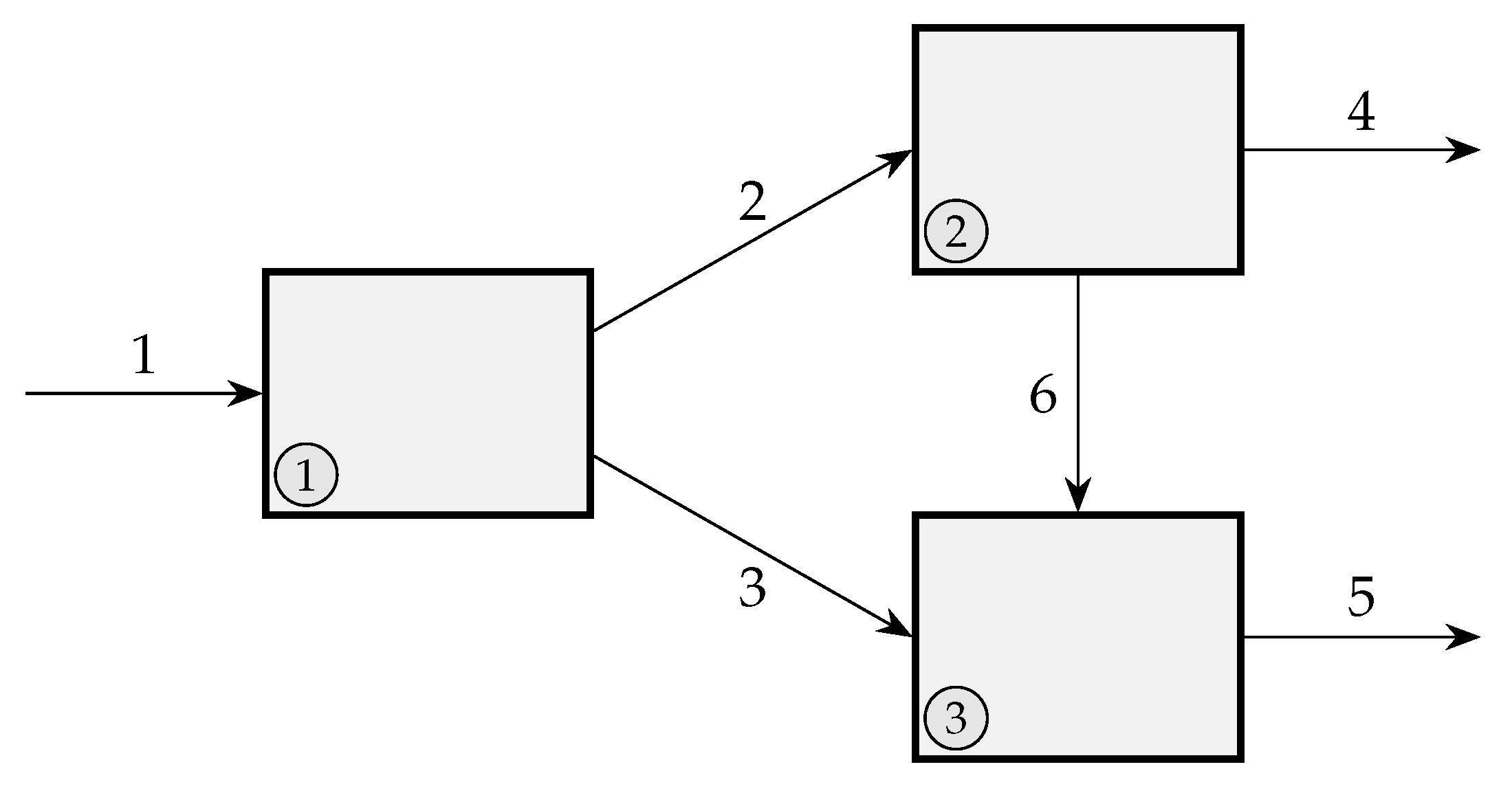
In general, the disaggregation of the process in Figure 4 can be described by the following system of characteristic Equation (11):

$$\left\{\begin{array}{c}{E}_1=k_{12}{E}_2+k_{13}{E}_3\hfill \\ E_2=k_{24}{E}_4+k_{26}{E}_6\hfill \\ E_3=k_{35}{E}_5\hfill \\ E_4={\omega }_4(\mathrm{const}.)\hfill \\ E_5={\omega }_5(\mathrm{const}.)\hfill \\ E_6=k_{65}{E}_5\hfill \end{array}\right.\mathrm{or}\left\{\begin{array}{c}{E}_1=\left({\displaystyle \frac{\partial E_1}{\partial E_2}}\right)E_2+\left({\displaystyle \frac{\partial E_1}{\partial E_3}}\right)E_3\hfill \\ E_2=\left({\displaystyle \frac{\partial E_2}{\partial E_4}}\right)E_4+\left({\displaystyle \frac{\partial E_2}{\partial E_6}}\right)E_6\hfill \\ E_3=\left({\displaystyle \frac{\partial E_3}{\partial E_5}}\right)E_5\hfill \\ E_4={\omega }_4(\mathrm{const}.)\hfill \\ E_5={\omega }_5(\mathrm{const}.)\hfill \\ E_6=\left({\displaystyle \frac{\partial E_6}{\partial E_5}}\right)E_5\hfill \end{array}\right.$$

(11)

Subsequently, according to the rule of the chain of the derivatives, the following expressions are obtained:

$$\left\{\begin{array}{c}\left({\displaystyle \frac{\partial E_0}{\partial E_1}}\right)=1\hfill \\ \left({\displaystyle \frac{\partial E_0}{\partial E_2}}\right)=\left({\displaystyle \frac{\partial E_0}{\partial E_1}}\right)\left({\displaystyle \frac{\partial E_1}{\partial E_2}}\right)\hfill \\ \left({\displaystyle \frac{\partial E_0}{\partial E_3}}\right)=\left({\displaystyle \frac{\partial E_0}{\partial E_1}}\right)\left({\displaystyle \frac{\partial E_1}{\partial E_3}}\right)\hfill \\ \left({\displaystyle \frac{\partial E_0}{\partial E_4}}\right)=\left({\displaystyle \frac{\partial E_0}{\partial E_2}}\right)\left({\displaystyle \frac{\partial E_2}{\partial E_4}}\right)\hfill \\ \left({\displaystyle \frac{\partial E_0}{\partial E_5}}\right)=\left({\displaystyle \frac{\partial E_0}{\partial E_3}}\right)\left({\displaystyle \frac{\partial E_3}{\partial E_5}}\right)+\left({\displaystyle \frac{\partial E_0}{\partial E_6}}\right)\left({\displaystyle \frac{\partial E_6}{\partial E_5}}\right)\hfill \\ \left({\displaystyle \frac{\partial E_0}{\partial E_6}}\right)=\left({\displaystyle \frac{\partial E_0}{\partial E_2}}\right)\left({\displaystyle \frac{\partial E_2}{\partial E_6}}\right)\hfill \end{array}\right.\mathrm{or}\left\{\begin{array}{c}{k}_1^{*}=1\hfill \\ k_2^{*}=k_1^{*}{k}_{12}\hfill \\ k_3^{*}=k_1^{*}{k}_{13}\hfill \\ k_4^{*}=k_2^{*}{k}_{24}\hfill \\ k_5^{*}=k_3^{*}{k}_{35}+k_6^{*}{k}_{65}\hfill \\ k_6^{*}=k_2^{*}{k}_{26}\hfill \end{array}\right.$$

(12)

Equation (2) can be rewritten in the matrix form:

$$\mathbf{E}=\left[\mathbf{K}\right]\mathbf{E}+\mathsf{\Omega }$$

(13)

where $\left[\mathbf{K}\right]$ is the matrix of unit consumption’s, and $\mathsf{\Omega }$ the vector of system’s outputs values, and Equation (8) becomes:

$${\mathbf{k}}^{*}={}^{\mathsf{t}}\left[\mathbf{K}\right]{\mathbf{k}}^{*}+{\mathbf{k}}_0^{*}$$

(14)

where ${\mathbf{k}}_0^{*}$ is the unit cost of the system’s input flows. In the analyzed case, these matrix variables are:

$$\left[\mathbf{K}\right]=\left[\begin{array}{cccccc}0& k_{12}& k_{13}& 0& 0& 0\\ 0& 0& 0& k_{24}& 0& k_{26}\\ 0& 0& 0& 0& k_{35}& 0\\ 0& 0& 0& 0& 0& 0\\ 0& 0& 0& 0& 0& 0\\ 0& 0& 0& 0& k_{65}& 0\end{array}\right]\mathsf{\Omega }=\left[\begin{array}{c}0\\ 0\\ 0\\ {\omega }_4\\ {\omega }_5\\ 0\end{array}\right]{\mathbf{k}}_0^{*}=\left[\begin{array}{c}1\\ 0\\ 0\\ 0\\ 0\\ 0\end{array}\right]$$

Please note that the matrix of the unit consumption $\left[\mathbf{K}\right]$ is common and transposed between Equations (13) and (14). Equation (13) is the primal model of the structure and Equation (14) is its dual model. Every productive structure or linear input–output interpretation of a system exhibits a primal representation with a corresponding single dual and vice versa [21].

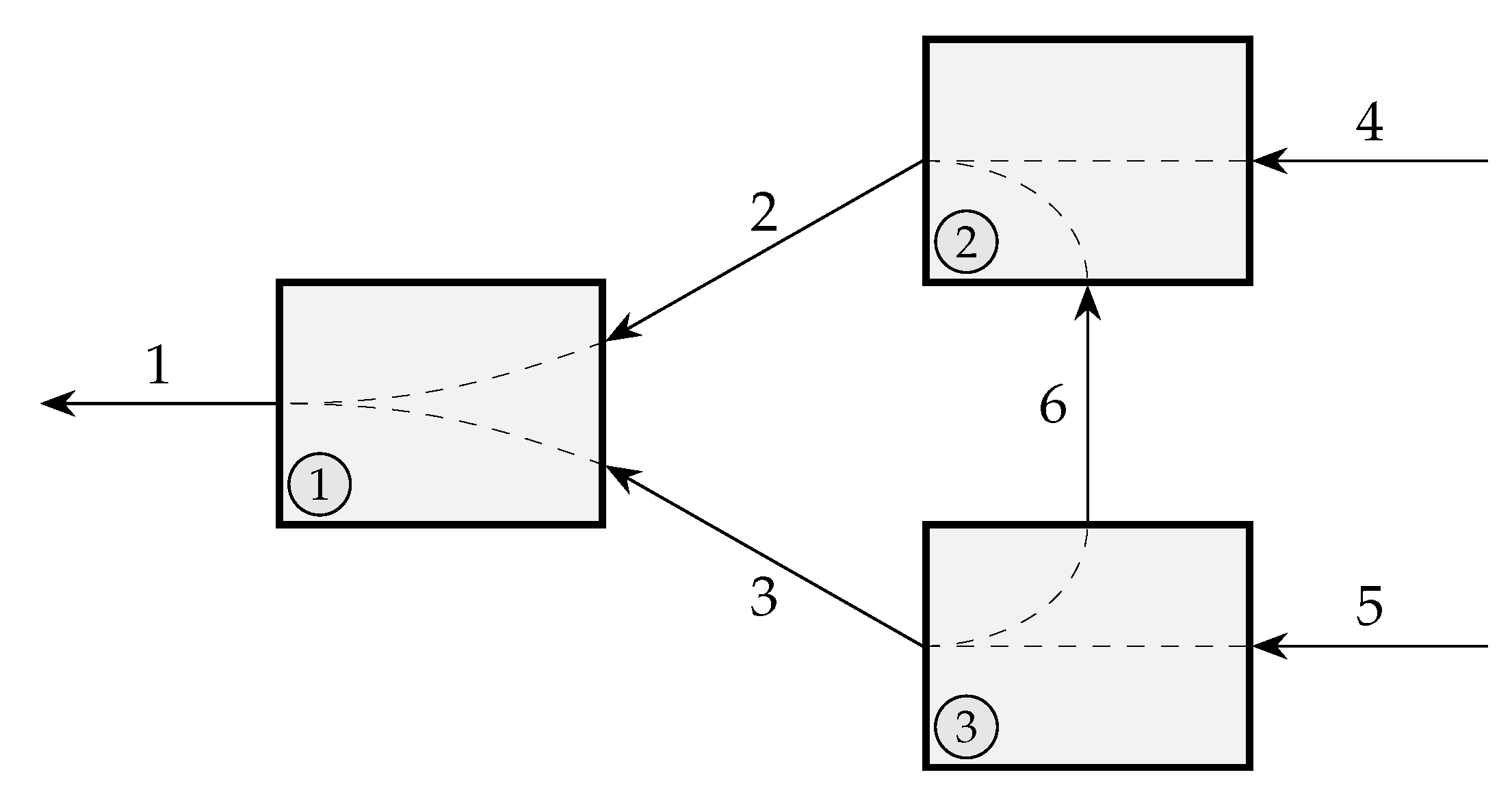
Figure 5 shows the dual cost structure of system in Figure 4. While the arrows in the productive process (primal) point from the resources toward the products, the cost structure (or dual) point from the products toward the resources. The costs search for the origin (causa materialis), while the products search for the final objective (causa finalis). [22].

The cost of the productive structure is a conservative property, this is to say, the cost of the inputs of any component are entirely transferred among its outputs Equation (15). It is a mathematical consequence of the founded hypotheses:

$$\sum _{i\in {\mathcal{E}}_u}{E}_i^{*}=\sum _{j\in {\mathcal{S}}_u}{E}_j^{*}$$

(15)

For instance, the case of component #1 is chosen, and the input equation:

$$E_1=k_{12}{E}_2+k_{13}{E}_3$$

is combined with its output equations $k_2^{*}=k_{12}{k}_1^{*}$ and $k_2^{*}=k_{12}{k}_1^{*}$, consequently:

$$k_1^{*}{E}_1=k_2^{*}{E}_2+k_3^{*}{E}_3$$

In general, applying Equations (2) and (8) to Equation (15) the cost balance is satisfied:

$$\sum _{i\in {\mathcal{E}}_u}{k}_i^{*}{E}_i=\sum _{i\in {\mathcal{E}}_u}{k}_i^{*}\sum _{j\in {\mathcal{S}}_u}{k}_{ij}{E}_j=\sum _{j\in {\mathcal{S}}_u}\left(\sum _{i\in {\mathcal{E}}_u}{k}_i^{*}{k}_{ij}\right)E_j=\sum _{j\in {\mathcal{S}}_u}{k}_j^{*}{E}_j$$

(16)

and the cost balance for the global plant, will be:

$$E_0=\sum _{i\in {\mathcal{E}}_0}{k}_i^{*}{E}_i$$

(17)

Therefore, the plant’s incidence matrix $\mathbf{A}$, can be defined as:

$$a_{ij}=\left\{\begin{array}{cc}\phantom{-}1\hfill & \mathrm{if}j\in {\mathcal{E}}_i\hfill \\ -1\hfill & \mathrm{if}j\in {\mathcal{S}}_i\hfill \\ \phantom{-}0\hfill & \mathrm{otherwise}\hfill \end{array}\right.$$

(18)

hence, the analyzed case can be described as follows:

$$\mathbf{A}=\left[\begin{array}{cccccc}\hfill 1& \hfill -1& \hfill -1& \hfill 0& \hfill 0& \hfill 0\\ \hfill 0& \hfill 1& \hfill 0& \hfill -1& \hfill 0& \hfill -1\\ \hfill 0& \hfill 0& \hfill 1& \hfill 0& \hfill -1& \hfill 1\end{array}\right]$$

In general, the following expression holds:

$$\mathbf{A}·{\mathbf{E}}^{*}=\mathbf{0}$$

(19)

and Equation (19) shows the cost conservation rule. It is a mathematical consequence of the founded hypotheses.

This result is quite remarkable because the following equations summarize straightforwardly the equilibrium thermodynamics for open systems:

$$\begin{array}{cccc}\hfill & \mathbf{A}·\mathbf{M}=\mathbf{0}\hfill & \hfill & \mathrm{Mass}\mathrm{Balance}\hfill \end{array}$$

(20)

$$\begin{array}{cccc}\hfill & \mathbf{A}·\mathbf{H}=\mathbf{0}\hfill & \hfill & \mathrm{Energy}\mathrm{Balance}\hfill \end{array}$$

(21)

$$\begin{array}{cccc}\hfill & \mathbf{A}·\mathbf{Ex}=\mathbf{I}\hfill & \hfill & \mathrm{Exergy}\mathrm{Balance}\hfill \end{array}$$

(22)

$$\begin{array}{cccc}\hfill & \mathbf{A}·{\mathbf{Ex}}^{*}=\mathbf{0}\hfill & \hfill & \mathrm{Cos}\mathrm{t}\mathrm{Balance}\hfill \end{array}$$

(23)

where $\mathbf{M}$, $\mathbf{H}$ and $\mathbf{Ex}$ are the mass, enthalpy and exergy vectors of the material streams: $m_i$, $m_i{h}_i$ and $m_i(h_i-T_0{s}_i)$; if there are the heat flows: zero, Q and $Q(1-T_0/T)$; and zero, W, W if there are working flows, respectively. Note the parallelism with respect the balance cost Equation (19). The presented structural theory explains the previously presented exergy cost theory.

4. Outcomes

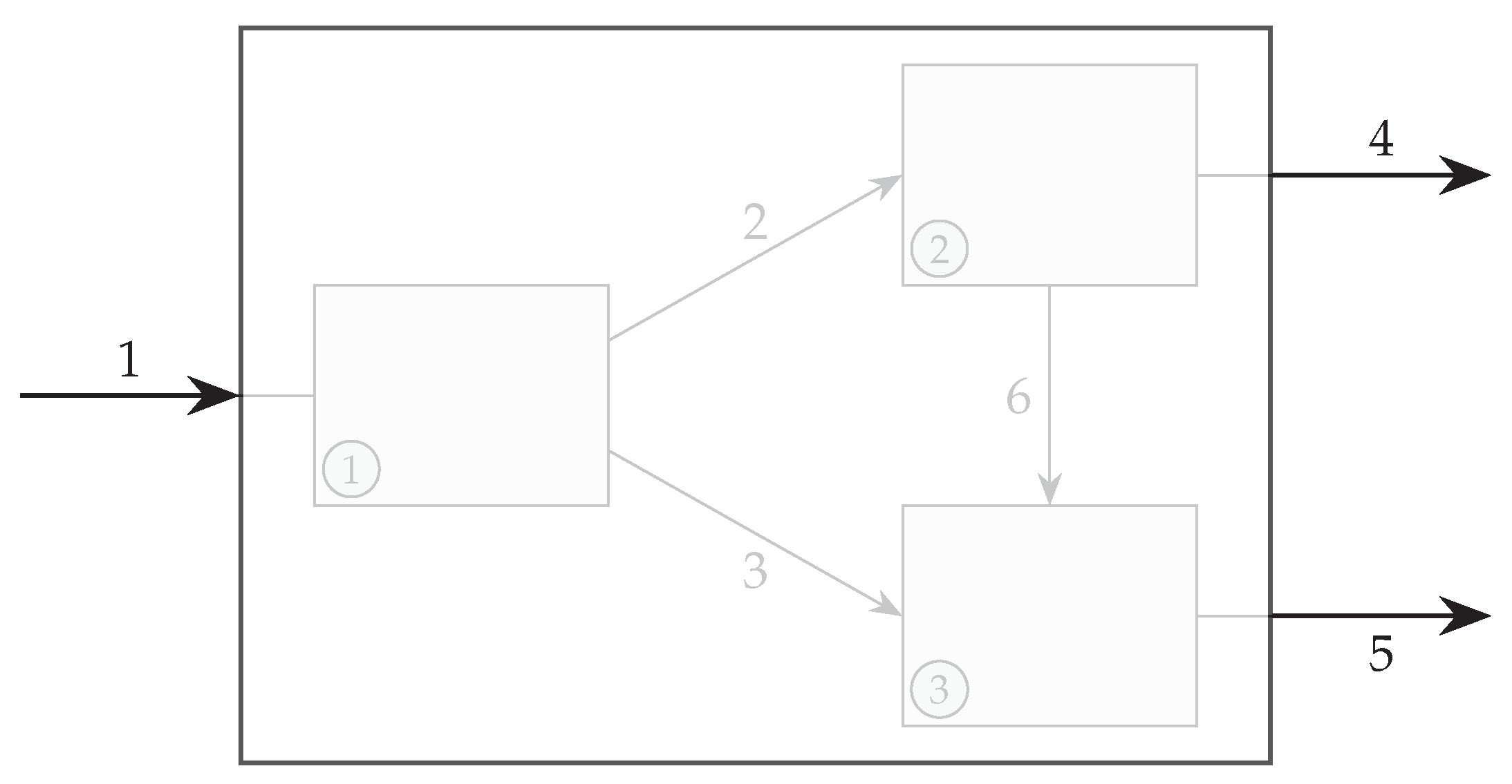
The presented theory mitigates several important deficiencies of the conventional exergy costing theories. First, its results do not depend on a disaggregation scheme. For example, the system in Figure 4 is aggregated into a single component Figure 6.

The physical behavior of the system remains (if linearized) the same under Equations (1) and (2). However, neither the Rule P or F can be applied between streams #4 or #5. In other words, $k_4^{*}$ is not equal to $k_5^{*}$, nor to $k_1^{*}$. Therefore, the theory provides many hints how to explore the cost relationships and suggests that greater disaggregation schemes are required.

The main idea originates from the difference between the characteristic equation, and the efficiency equation (e.g., Figure 2 or Figure 3). The former reflects the physical behavior of the component while the second is a definition, (i.e., an identity). For instance, the linear characteristic equation of Figure 6 is expressed as follows:

$$E_1=k_{14}{E}_4+k_{15}{E}_5,$$

meanwhile, its efficiency equation could be of the following type:

$$E{x}_1\equiv kE{x}_4+E{x}_5$$

The similarity is evident; however, the more the analyst aggregates, the more deviates the physical behavior of the system from the aggregated efficiency definition. Note also that the reference environment of the exergy depends on the practitioner choice, whereas Equation (2) should be independent.

The structural theory, first presented in [14,23], has been largely ignored in the study of different alternate rules for costing allocations, such as in the allocation of the costs of wastes or by-products. This might be due to the difficulties of determining the fundamental equations of components as in Equation (1) or their linearized equations, Equation (2). Rather, the theory has been used to check the logic of rules F and P.

Please note that Odum’s Emergy Analysis [24,25] does not satisfy Equation (19) because it considers that when a biological system produces simultaneously two products, the same amount of solar energy is required for each product. This does not deny the idea of emergy; it simply states that this is not a regular cost.

In the same way, a non-linear theory does not satisfy Equation (4) because the primal would be of the following type:

$$d{E}_i=\sum _j\left({\displaystyle \frac{\partial E_i}{\partial E_j}}\right)d{E}_j,$$

(24)

rather than as Equation (19). However, Equation (24) enables a generalization of the theory, For example, in [23], the costs are the Lagrange multipliers of an optimization of the plant.

The structural theory formally relates to the input–output theory [20]; however, the characteristic equation makes the difference because it deeply connects the thermodynamic behavior of an energy system to the stream costs such as in a transparent box. Instead of the economic performance of highly aggregated economy sectors, their input–output flows are obtained outside the black boxes, which constitute each sector of the economy. In addition, the second law exergy analysis appears as a natural connection between physical behavior and cost, because it locates and accounts for irreversibilities occurring in a plant; thus, it relates the physical losses to the costs. Please note that “cost” is a concept that originates from economics, while “irreversibility” originates from thermodynamics. The structural theory can be considered a sought-after bridge between classical economics and physics. Thus, we consider the term “thermoeconomics” is more appropriate than alternatives such as exergoeconomics [17].

5. Drawbacks of Exergy?

One important result of the structural theory is that any energy function of the type $E=H-T_{x}S$, may be used to assess different sets of costs. Thus, why should exergy that uses a fixed $T_0$ instead of a variable $T_x$ be considered? The most important objective of this study is to question the exergy directly to assess costs.

Mythologizing exergy is not convenient, it only measures the number of times that a product is potentially equivalent to another. Therefore, the kilograms of natural gas; mass of steam at a certain temperature and pressure; and kinetic, magnetic, or mechanical energies are possible units for measuring exergy. Certainly, it does not reflect the product value. A broken glass has practically the same exergy as a new one, and the exergy of gold at $T_0$ is zero as taken by reference. Moreover, everybody would prefer 1 g diamond than 1 g pure graphite, even though they practically have the same exergy.

In addition, the manufacture of a continuous and broken thread costs the same exergy although the latter would not be saleable. Exergy reduces a probably irreducible object to a single numerical value. The color, taste, form, texture, or artistic impression (i.e., properties that human beings value) have no distinguishable exergy. The exergy and exergy cost are only a measure of reality, which should not supplant other possible analyses.

Can the concept of value be assessed by thermodynamics? Does it make sense to go beyond the exergy cost when it comes to knowing the cost of objects? It has been claimed many times that exergy is a measure of the quality of things, which is false; it is a measure of the energy imbalance that a system has with respect to a reference environment. It is a measure of the thermodynamic quality of energy and not of objects. Moreover, the quality specification is much more complex. A dose of carbon monoxide may have the same exergy as a certain amount of food; however, everybody knows which one to ingest or burn in a boiler. The same food can present a disgusting or an extraordinary aspect and contain the same amount of exergy. Based on the many possible examples, it seems strange to confuse exergy with quality.

Assessing thermodynamic quality requires many specifications such as the pressure, temperature, composition, height, and speed. Quality also depends on the context, whereas exergy does not. In general, thermodynamic equivalence is not a measure of the equivalence of values. Even circumstances and the moment make a thing seem more or less valuable. Researchers should distance themselves from neo-energeticism (or even better “exergeticism”), which regards exergy rather as a measure of the value of objects than as their monetary value. The exergy and exergy costs provide complementary information on the human footprint on Earth; ignoring them is as dangerous as extolling them as a unique instrument for managing the natural resources and environment.

Furthermore, the second law has not exhausted its message regarding exergy. The following equation:

$$F-P=I+R$$

(25)

identifies product, waste, and what is (or is not) a usable resource. Certainly, every real-world process experiences an irreversibility. The Gouy–Stodola theorem relates the entropy generation to irreversibility:

$$I=T_0{S}_g$$

(26)

Regardless of the way the quality of every stream, product, or service is defined (generalized exergy function), it is easier to identify the quantity. Thus, the magnitude of a property X is always a product of its quantity $q_x$ multiplied by its specific quality x:

$$X=q_x·x$$

(27)

It would be interesting to determine the amount of resources required to compensate for a deterioration of any component in a constant production for a set of quality specifications for each flow interacting in a system.

6. The Relative Free Energy Function

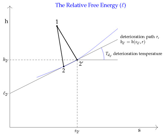
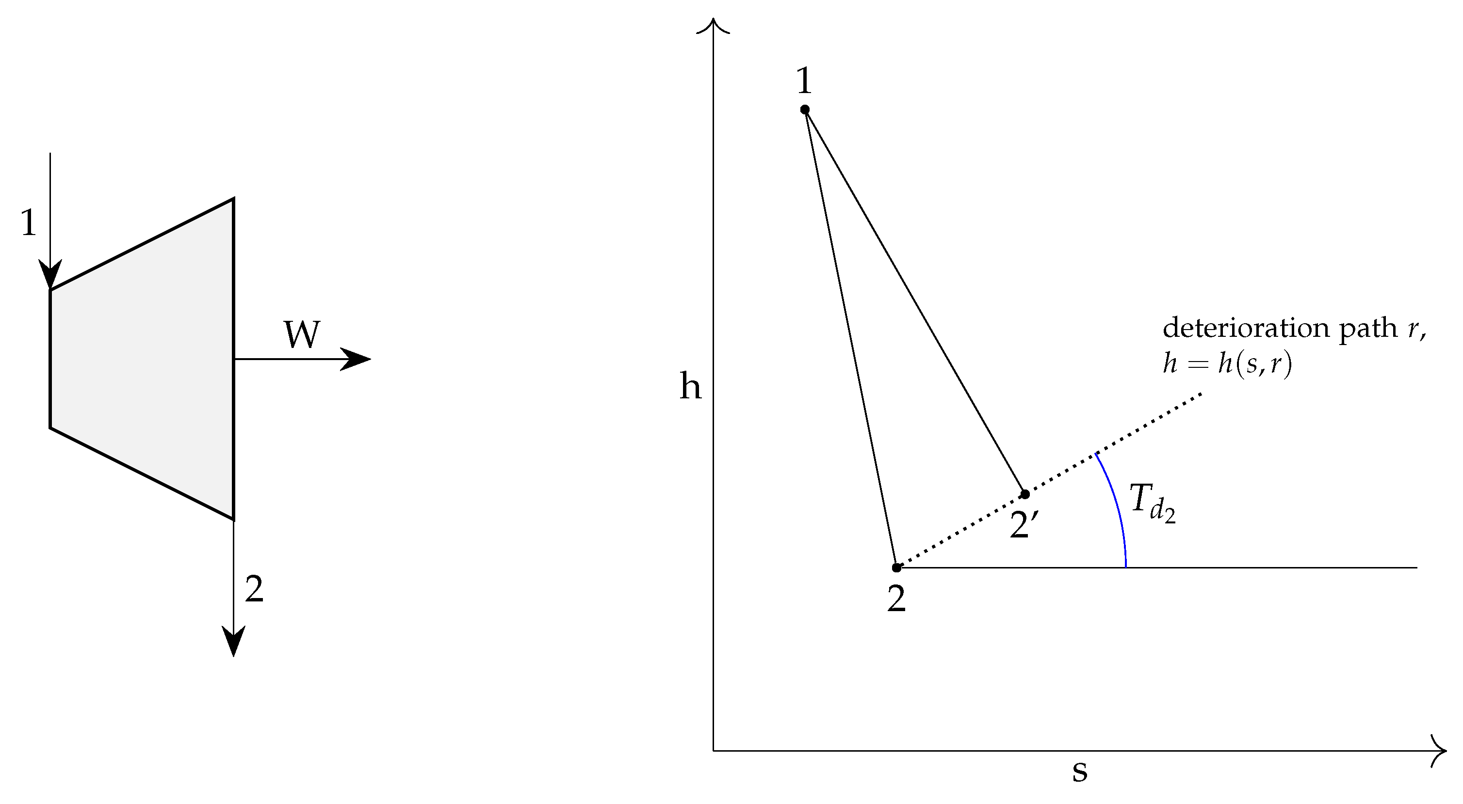
Before generalizing the problem, a simple case should be analyzed: for example, the expanding flow of a turbine produces work on the shaft. In an $(h,s)$ diagram, Figure 7, the actual process evolves from state 1 to state 2.

The energy and entropy balances of the process (first and second laws) are as follows:

$$\begin{array}{cc}\hfill W=& m\left(h_1-h_2\right)\hfill \end{array}$$

(28)

$$\begin{array}{cc}\hfill S_g=& m\left(s_2-s_1\right)\hfill \end{array}$$

(29)

If the turbine degrades, at a rate equal to the specifications of the inflow #1, an increase in the entropy generation evidently results in an increase in the amount of entering fuel (path 1) to keep the production constant. Owing to the degradation, the new state of the outflow #2’ is characterized by ($h_{2^{\prime }}$, $s_{2^{\prime }}$).

A differential analysis under the conditions: W=const., $h_1$=const., and $s_1$=const., leads to the following expressions:

$$\begin{array}{cc}\hfill \left(h_1-h_2\right)dm& =md{h}_2\hfill \end{array}$$

(30)

$$\begin{array}{cc}\hfill \left(s_2-s_1\right)dm+md{s}_2& =d{S}_g\hfill \end{array}$$

(31)

Subsequently, if the deterioration temperature of flow #2 is defined as a quotient:

$$T_{d_2}\equiv d{h}_2/d{s}_2$$

the result is as follows:

$${\left(\frac{dm}{d{S}_g}\right)}_r=\frac{T_{d_2}}{\left(h_1-h_2\right)-T_{d_2}\left(s_1-s_2\right)},$$

(32)

where r is the deterioration path, as it shown is Figure 7.

Equation (32) is the mathematical expression of the existing relationship between any local degradation and the increase in associated resources if the production of the component should remain constant.

These equations and the function $\ell \equiv (h_1-h_2)-T_d(s_1-s_2)$ were presented in [11]. Valero called it the relative free energy [26,27], and $T_d$ the deterioration temperature (In 1994, Prof E. Sciubba proposed to name it “dissipation” temperature. However, the authors consider the word “deterioration” more precise, since that word always relates to a component rather than to a process).

The expression “relative free energy” (RFE) originates from its similarity to the Gibbs free energy function. Equation (32) states that any deterioration process in an energy component has an associated $T_d$ in the exit stream of supplying fuel. This parameter possesses temperature dimensions even if it is not a gauging temperature; it can be calculated by measuring the quotient $d{h}_2/d{s}_2$ experienced by the output stream of the component’s fuel.

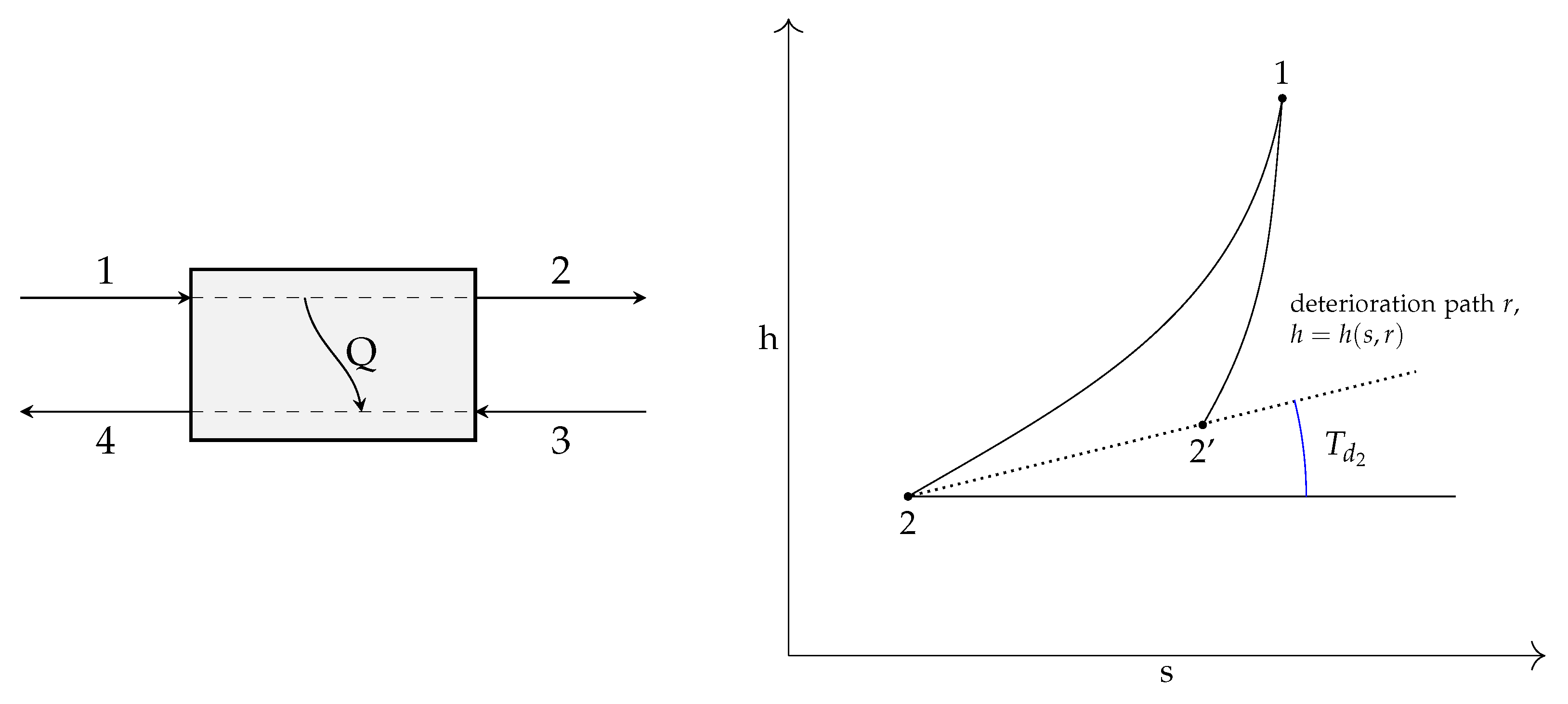
The heat exchanger Figure 8 experiences the same procedure. In that case, the enthalpy and entropy balances are written as follows:

$$\begin{array}{cc}\hfill m_1\left(h_1-h_2\right)-m_3\left(h_4-h_3\right)& =0\hfill \end{array}$$

(33)

$$\begin{array}{cc}\hfill m_1\left(s_1-s_2\right)-m_3\left(s_4-s_3\right)& =-S_g\hfill \end{array}$$

(34)

If the heat source degrades, at equal to the specifications of the inflow #1, an increase in the entropy generation results evidently in an increase in the amount of entering fuel #1 to maintain a constant production; thus, $m_3$, $(h_3,s_3)$, and $(h_4,s_4)$ are constant. Owing to the degradation, the new state of outflow #2’ is characterized by $(h_{2^{\prime }},s_{2^{\prime }})$.

A differential analysis under the condition $(h_1,s_1)$ are constant, leads to:

$$\begin{array}{c}\hfill \left(h_1-h_2\right)d{m}_1=m_{1}d{h}_2\end{array}$$

(35)

$$\begin{array}{c}\hfill d{S}_g+\left(s_1-s_2\right)d{m}_1=m_{1}d{s}_2\end{array}$$

(36)

If the dissipation temperature of flow #2 is defined as a quotient:

$$T_{d_2}\equiv \frac{d{h}_2}{d{s}_2}>0$$

subsequently Equation (32) is also satisfied.

According to the second law, $d{S}_g$ is always positive; therefore, more fuel must be used to obtain the same product, and $dm>0$. Because $T_{d,2}$ is positive, the term $(h_1-h_2)-T_{d,2}(s_1-s_2)$ must be positive; in other words, $T_{d,2}(s_1-s_2)$ is always lower than $h_1-h_2$. Also note that in a low pressure steam turbine of a Rankine cycle, $T_{d,2}$ coincides with the condenser temperature which is fully logical. More examples could be found in [27].

7. h-s Deterioration(s) Path(s) of an Energy System

Man-made energy systems transform the energy flows into other flows with a purpose. Commonly, the name of a component describes its function: a boiler boils water, a condenser condenses steam, and a heat exchanger exchanges heat. The understanding of how nature behaves is the basis of the component design. The entering flow performs a purposive path through which its thermodynamic properties change progressively until the flow exits the component. This path is never strictly determined, either because of possible changes in the quantity/quality of the entering flow or because of changes in the behavior of the component itself. This path variation results in a change in the properties of the exiting flow with respect to its design conditions. There are as many new exit states as causes of change, which are called “malfunctions” and are classified into two categories: intrinsic and induced [28,29,30]. The term “intrinsic” refers to the internal deterioration of the component; the term “induced” refers to its off-design conditions (not the optimal operating conditions). A good component design foresees most of these off-design conditions. Literature and some manufacturers provide governing equations and control parameters based on semi-empirical models of the machines.

For a given deterioration cause r of an energy component, either intrinsic or induced, a geometric path in the $h-s$ plane of the possible exit flow states can be identified. Let $h_{2^{\prime }}=h_{2^{\prime }}(s_{2^{\prime }},r)$ to be the function describing this dissipation path of the exiting flow, as in Figure 7, where:

• $1⟶2:$ is the design path of the stream in the component.
• $1⟶2^{\prime }:$ is the stream path after the component deterioration.
• $2⟶2^{\prime }:$ is the dissipation path of the exiting stream $h_{2^{\prime }}=h_{2^{\prime }}(s_{2^{\prime }},r).$

The function $h_{2^{\prime }}=h_{2^{\prime }}(s_{2^{\prime }},r)$) can be regarded as the mathematical description of the effects on the exiting flow caused by the component deterioration cause r. This function always exists for a given differential malfunction interval. Moreover, under actual machine conditions, this function is a composite curve of the different paths caused by the concurrent deteriorations acting simultaneously on the component [28]. The next section focuses on this function.

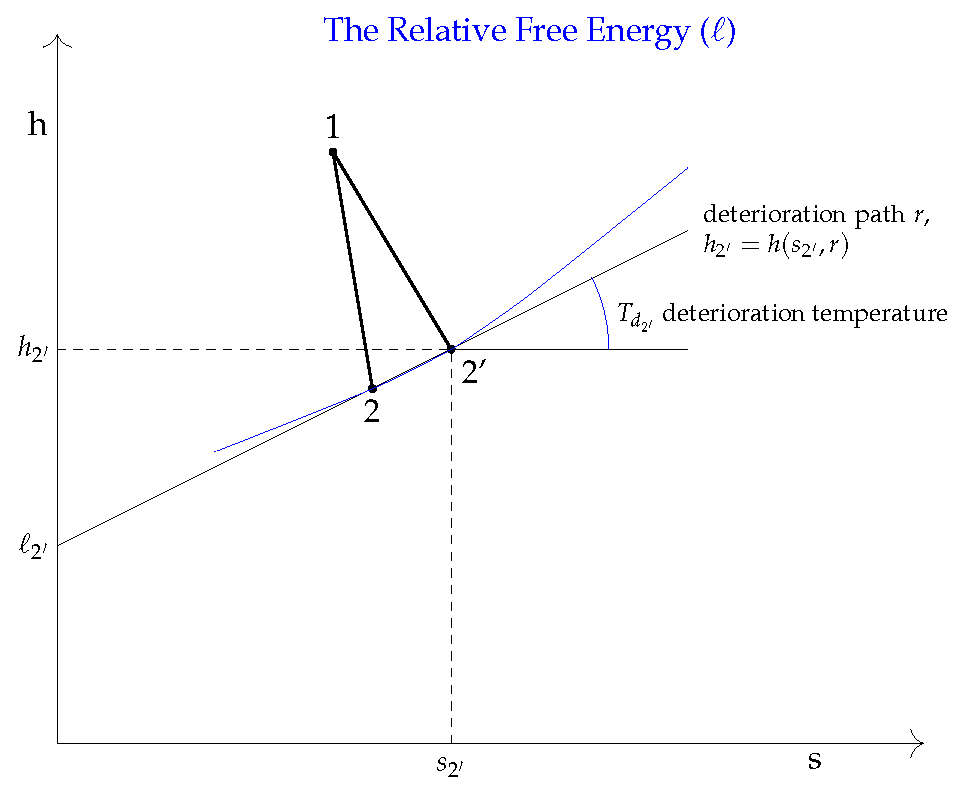
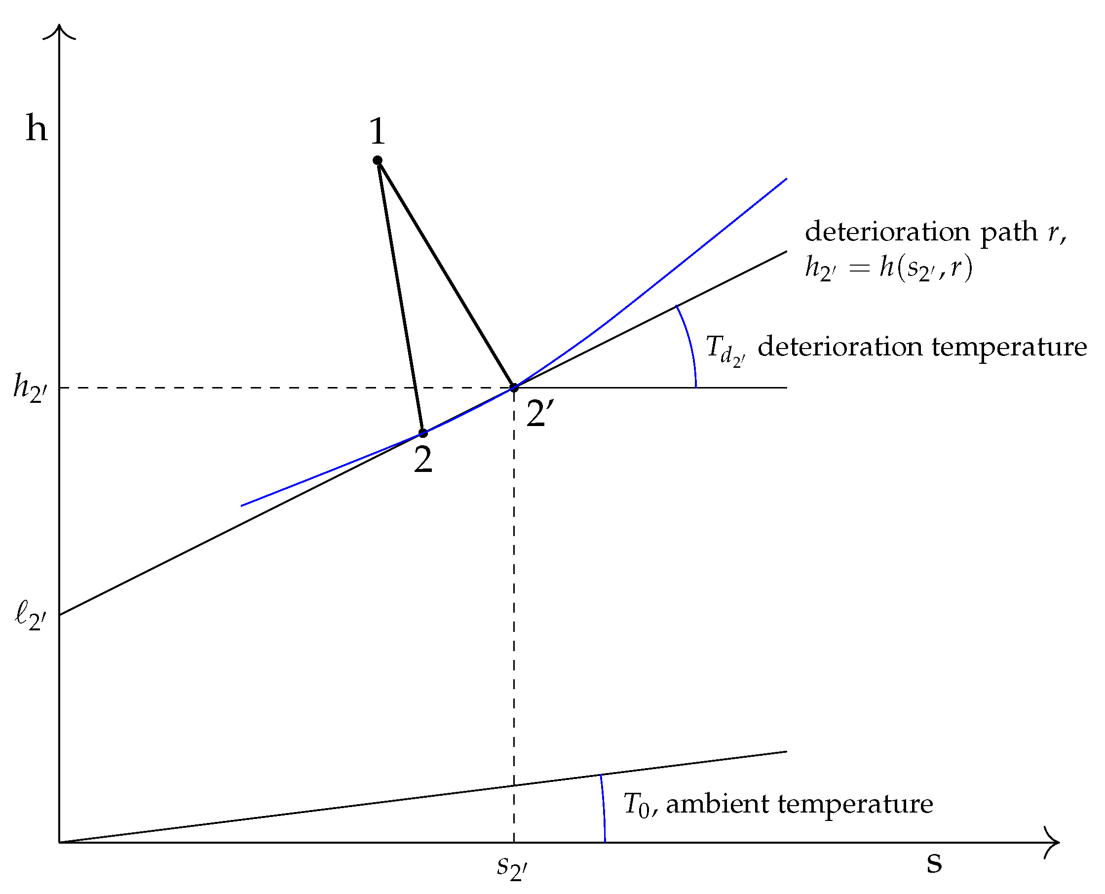
8. The Legendre Transform of a Deterioration Path

For each deterioration cause, r, the existence of a function $h=h\left(s\right)$ of the exiting flow can be assumed, which can be described in the $h-s$ plane with the conventional point geometry or Plücker line geometry for strictly convex functions as a convolution of the tangents of the original curve. This technique is named the Legendre transform of the function $h=h\left(s\right)$ and is widely used in classical thermodynamics [31,32]. As it is shown in Figure 9, the intersection of the tangent line of the deterioration path r with the h- axis is ℓ and its slope is $T_d$:

$$T_d=\frac{h-\ell }{s}$$

or

$$\ell =h-T_{d}s\mathrm{i}.\mathrm{e}.,\ell =\ell \left(T_d\right)$$

(37)

Equation (37) is the Legendre transform of the deterioration path $h_{2^{\prime }}=h_{2^{\prime }}(s_{2^{\prime }},r)$. In fact, pairs of $({\ell }_{2^{\prime }},T_{d,2^{\prime }})$ for each exit state, #2’, of the component provide the same information as pairs $(h_{2^{\prime }},s_{2^{\prime }}$). Since the relationship ${\ell }_{2^{\prime }}={\ell }_{2^{\prime }}\left(T_{d,2^{\prime }}\right)$ is mathematically equivalent to the relationship $h_{2^{\prime }}=h_{2^{\prime }}(s_{2^{\prime }},r)$, it can also be considered the description of the deterioration path. More in general, $h_r=h_r\left(s_r\right)$, is the deterioration function in the h-representation; whereas ${\ell }_r={\ell }_r(T_d,r)$ is the deterioration function in the ℓ-representation. In other words, ${\ell }_r$ and $T_{d,r}$, are inseparable in a deterioration path, r, such as $h_r$ and $s_r$ do. Note also that h and s do not represent absolute values because they refer $h_0$ and $s_0$ values. Unless otherwise stated h and s represent $h-h_0$ and $s-s_0$.

According to the definition of relative free exergy Equation (37), expression Equation (32) could be written as:

$${\left(\frac{dm}{d{S}_g}\right)}_r=\frac{T_d}{{\ell }_1-{\ell }_2}$$

(38)

The deterioration temperature, $T_d$, is not a physical temperature, it is a parameter and derivative with temperature dimensions:

$$T_d={\left(\frac{dh}{ds}\right)}_r$$

(39)

It can be interpreted as the entropic cost of the deterioration. The greater $T_d$, the lower the relative free energy of the exiting flow. Well-known contributors to technical thermodynamics such as Baehr [12] have defined the “friction work” or “loss work” for an expander as follows:

$$d{W}_r=T_{d}d{S}_g$$

(40)

This loss work is energy that has not been dissipated into the environment at $T_0$ and contributes to the degradation of the exiting flow of the expander. It increases the enthalpy and entropy of the exiting stream and reduces the work produced by the turbine, thereby decreasing its efficiency.

In the example of the turbine, Figure 7, a differential analysis of the exergy Equation (25) under the conditions $(h_1,s_1)$ and W constants, results in:

$$dF=dI=T_{0}d{S}_g$$

(41)

Therefore, the following expression is obtained:

$$dF=T_{0}d{S}_g=\frac{T_0}{T_d}d{W}_r$$

(42)

Another important antecedent was the work of Alefeld [13], who worked on heat pumps and refrigeration systems: he questioned the use of the reference ambient temperature $T_0$ instead of a variable temperature $T_x$ associated with the whole system. In particular, he proposed for the case of a Rankine cycle, where this temperature $T_x$ be equal to that of the condenser vacuum, $T_{vac}$. Alefeld was highly criticized by the community of exergy practitioners, because the holistic vision that exergy provides was lost in his proposal. This article is a recognition to his work because mathematical proofs are stronger than reasonable assumptions.

The relative free energy function, ℓ, represents the local free energy conditioned by the deterioration path, r. It is an intensive property, and its corresponding extensive property:

$$𝓛=m\ell$$

(43)

is the amount of energy of the exiting stream in a fuel of the type $E_1-E_2$, which is not affected by the deterioration of the component. This is because when the exit flow changes its state owing to the deterioration, h and s, vary by following the path $h_r=h_r\left(s_r\right)$. Consequently, the following expression is obtained:

$$d{\ell }_2=d{h}_r-{\left(\frac{dh}{ds}\right)}_{r}d{s}_r=0\mathrm{or}{\ell }_2=\mathrm{const}.$$

(44)

In addition, the function $h_r=h_r\left(s_r\right)$ is neither a straight curve nor a slope $T_0$. Therefore, ℓ, exceptionally coincides with the specific exergy of the stream, and the exergy increase in the output stream in the turbine is: $e{x}_{2^{\prime }}-e{x}_2=(h_{2^{\prime }}-h_2)-T_0(s_{2^{\prime }}-s_2)$.

In the example of the turbine, $(h_1,s_1)$ and W are constant, then applying differential analysis to the unit exergy consumption definition: $k\equiv F/P$, it follows:

$$dF=Pdk$$

(45)

Combining both Equations (41) and (45):

$$dk=\frac{T_{0}d{S}_g}{W}=\frac{T_0}{T_d}·\frac{T_{d}d{S}_g}{W}$$

(46)

and applying Equation (38), it follows:

$${\left(\frac{dk}{dm}\right)}_r=\frac{T_0}{T_d}·\frac{{\ell }_1-{\ell }_2}{W}$$

(47)

This expression is quite important, because it relates the loss of exergy efficiency in the turbine with the additional mass of fuel to compensate it at constant production. In other words, it relates the malfunction of the turbine with the need for more entering fuel. Also, this expression opens the way of changing the paradigm of exergy by relative free energy.

Therefore, a new definition of the efficiency (or its inverse specific consumption) of the turbine appears:

$$k_L=\frac{F_L}{P_L}=\frac{{𝓛}_1-{𝓛}_2}{W}=\frac{H_1-H_2-T_d\left(S_1-S_2\right)}{W}$$

(48)

This new definition of efficiency of the turbine has the important property that if the turbine malfunction following a r path, its characteristic equation becomes:

$${𝓛}_1={𝓛}_2+k_{L}W+\mathrm{const}.$$

(49)

this constant might be selected as the standard reference state for h and s calculations $(h_0,s_0)$.

When a malfunction in the turbine follows a trajectory r at W constant, it follows:

$${\ell }_{1}dm={\ell }_{2}dm+Wd{k}_L$$

(50)

because ${\ell }_1-{\ell }_2$ is constant along trajectory r. Therefore:

$$\frac{d{k}_L}{k_L}=\frac{dm}{m}$$

(51)

in other words, any additional percentage of malfunction following a trajectory r at W constant result in an additional percentage of mass of fuel entering the turbine.

Also note that exergy does not fulfill Equation (51), because:

$$e{x}_{1}dm=e{x}_{2}dm+mde{x}_2+Wdkde{x}_2\ne 0$$

Equation (49) is not a mere efficiency definition, as it is the unit exergy consumption definition $k\equiv F/P$. It corresponds to a physical description of the turbine system and what is more important, it does not depend on the reference environment temperature $T_0$, but on the behavior of the turbine. The structural theory, as explained in this paper, together with the relative free energy function allows the obtaining of an interesting characteristic function of the behavior of thermodynamic systems. If under the structural theory, the coefficients $k_{ij}$ are the precursors of costs $k_j^{*}$, should these costs be their “natural” costs? or perhaps they should be named “regular” costs? In any case these costs are directly related to the additional amount of resources needed to compensate the malfunction.

The expression Equation (38) shows that the second law has not yet said the last word regarding the relationship between the thermodynamic quantity, quality, cost and irreversibility. In general, the reason of why $T_d$ instead of $T_0$, stems from the fact that the additional degraded energy not used in producing the product becomes part to the exiting streaming instead of going directly to the environment at $T_0$. The value of $T_d$ depends on how great the additional irreversibility is created. Such interpretation of $T_d$, allows understand that its lowest attainable value is $T_0$, while, apparently, has no highest limit.

In other words, the deterioration lowers the free energy of the exiting stream. As this deterioration always relates to some component, this is why we name this function relative free energy. In the same way that the Gibbs free energy relates to some chemical reaction, the RFE relates to some component deterioration in a system.

The key problem of diagnosis of energy systems stems in how to assess, as precisely as possible, the relationship between local irreversibilities and additional consumption of resources. At constant production, a local irreversibility needs additional resources to compensate it, but also modifies the exiting streams, affecting downstream enthalpies and entropies and eventually the upstream ones, if recycling. A certainty derives from the Second Law: Any inefficiency in a process increases the entropy generation. This means that any mechanical, thermal or chemical loss generates entropy and reduces efficiency. However, any efficiency decrease means more resources (at equal quality) to get the same product. If one knows the amount of local resources needed to compensate a local deterioration, r, i.e.,

$${\left(\frac{\partial m_{local}}{\partial S_g}\right)}_r$$

and knows how the global system’s resources is related with local resources, i.e.,

$${\left(\frac{\partial m_{global}}{\partial m_{local}}\right)}_r$$

one may have a new theory of energy system diagnosis. We will present this theory with due examples in a following paper; however, an early analysis was published in [33].

9. Conclusions

The definition of efficiency plays a fundamental role in the process of calculating average exergy costs. So, efficiency and cost became closely linked. In such a way, the theory of exergy cost [2,3] was extensively used to assess costs on many thermoeconomic/thermodynamic applications. However, the exergy cost depends on the plant disaggregation scheme. It is necessary to look after the cost formation process, by searching how much exergy has been consumed in the processes and where they have consumed it. The result of this activity is a given productive structure. However, if exergy depends on a chosen reference state, exergy efficiencies and their closely related costs will depend on such selection. Notwithstanding, any deterioration that increases entropy generation results in an additional expense of resources used to produce the same product. Both the entropy increase and the additional resources are measurable and free from analyst selections. Therefore, something fails in the conventional theory.

The use of exergy instead of enthalpy or the Gibbs function for obtaining costs increase the overall, coherent and systematic view of a set of stream costs in a productive structure. To what extent one could use these costs to assess component malfunctions? In other words, can average costs be used as marginal costs?

The exergy cost is the exergy backpack, embodied exergy or the exergy footprint of a commodity; in fact, Szargut named it as “cumulative exergy consumption”, [16] i.e., its “past” characterization (history), while exergy is the potential energy of such a commodity, or its remaining capacity for doing something else. Can average costs predict future degradations or only past irreversibilities?

The purpose of Thermoeconomics is to obtain a coherent and significant set of costs in a given structure. That is because its applications are directed towards the optimization and diagnosis of productive structures. Therefore, the costs of internal streams are quite important to analyze the behavior of the system. Consequently, internal costs ought to be as sensitive as possible to system degradation. A theory that would provide exact costs would be the objective of thermoeconomic diagnosis. In fact, one can obtain the costs of final products or commodities, without performing very detailed analyses. In other words, in no way Thermoeconomics, as it is already known, is far from being finished. Moreover, the analyst needs to look for the cost formation process of wastes, [18], not mentioned here even when some ideas developed here could be used to clarify it.

This paper presents a general theory of (linear) costing, demonstrating and answering questions like:

• To what extent the linear characteristic equation Equation (2) a component can be conformed to its efficiency definition, $F-kP=0$ ?
  In fact, exergy efficiency must be coherent with the component’s design purpose, but one designs machines by observing the behavior of nature. So what is first, efficiency or nature? We overcome this drawback with Equation (48).
• Why the F and P rules, or any other costing proposal may be either rational or not under a given disaggregation scheme.
• Under a set of conditions, we may say that the exergy costs balances are the mathematical dual of exergy balances and vice versa. The exergy cost and the exergy are like specular images of the same entity.
• A compact vision of current day thermoeconomics/exergoeconomics under the Equations (20)–(23).
• A costing theory applicable to any thermodynamic function like, enthalpy, exergy, Gibbs free energy or any other.
• In analyzing this last point, we proposed a new thermodynamic function, called the relative free energy, ℓ, and introduced a new parameter $T_d$ called deterioration temperature due to a component’s deterioration cause r, characterized by a thermodinamic trajectory $h=h(s,r)$ describing the effects on the exiting stream.
• The Legendre transform of the deterioration path, $h_2=h_2(s_2,r)$ is the relationship ${\ell }_2={\ell }_2(T_{d,2},r)$. In other words, the pairs ${\ell }_r$ and $T_{d,r}$, are so inseparable in a deterioration path, r, as the pairs $(h_r,s_r)$ do.
• The general formula (38) applies for different flowing streams in energy systems under each particular deterioration path, $r_i$. A given component may have several deterioration paths, not only one. Therefore, the concept of component malfunction need be associated with that of deterioration paths. Besides that, this formula can be applied to any system –under the defined conditions– no matter its aggregation level. Each degradation will have its deterioration temperature as well as its corresponding RFE efficiency.
• A way for assessing appropriate characteristic equations of thermal systems as it was obtained here for the case of turbines.
• As the component’s deterioration does not depend on the analyst’s decision on the chosen reference state, the deterioration temperature no longer depends on the chosen reference temperature. Neither does the new definition of efficiency using the RFE. This fact does not isolate the plant from environmental conditions, but eliminates the arbitrary selection of any reference state. That idea clarifies the role of the environmental conditions onto the plant.

The Exergy Cost Theory provides reasonable costs. Will relative free energy provide a set of natural (or perhaps named regular) costs? In fact, the cost of a deterioration is directly related to the physical behavior of that deterioration. This way it also means that these costs are in fact marginal costs, since they incorporate the future malfunction behavior of the component.

The theory sketched here opens new fields of knowledge, since new questions appear: Is exergy the best thermodynamic function when diagnosing systems? Why $T_0$ needs to be the same for each component of a given structure? Can we use this theory to assess objective average costs of deteriorations free from assumptions? The deterioration behavior of an energy system relates with internal marginal costs while exergy costs with history. Should we change our definitions of efficiency under the light of the relative free energy function? Etc. Even if described early in the 1990s, all these ideas are tools for future, [34]. Cost is a measure of expended resources to produce something, then, costing with the relative free energy instead of exergy would open a new field of a more precise theory of Thermoeconomics. We presently work in such ideas.