Testing of Electrical Energy Meters Subject to Realistic Distorted Voltages and Currents ^†

Abstract

This paper presents a study on revenue active electrical energy meters. The huge installation along the distribution network of these devices made them a key element for energy billing, but also for monitoring the grid status. Hence, it is evident that the relevance of guaranteeing a trusty metering performance, and consequently a proper standardization, is needed. The operation of the meters is regulated by standards harmonized with the European Directive 2014/32/EU (known as MID). Still, and not infrequently, compliance to some legacy standards is declared on the device specifications. Thus, a brief comparison between the latest standards is presented. In particular, the focus was set on evaluating the potential impact of the harmonic disturbances on the energy meter accuracy, since they are omnipresent in the modern power networks. The evaluation has been carried out on three off-the-shelf class B meters by means of a new test procedure that considers realistic and quasi-realistic harmonic disturbances. Such tests showed that realistic harmonic disturbances affect significantly only some energy meters. Therefore, the standards should not neglect this kind of scenario.

1. Introduction

The observability of the distribution network (low and medium voltage, LV and MV) is becoming a key-factor after the huge revolution of the grid towards the smart grid concept [1,2,3,4,5]. Effective control stability of the network and fair energy billing [6,7,8] are possible when accurate measurements of the energy consumed/generated by users/producers are collected by energy meters (EM). In addition, the knowledge of such critical quantities can be used to run several algorithms used to manage and control the network [9,10,11,12]. However, the measurement process performed by EMs is affected by the spread among the network of renewable energy resources and non-linear loads, which worsen the electric power quality (PQ), and hence the quantities to be measured by EMs.

Nowadays, electronic EMs are replacing the old electromechanical induction meters, even if their behavior is acceptable with medium–low levels of PQ [13]. The reason is that EMs are preferred because they enable utilities and consumers to perform “smart” operations, such as remote readings, computation of many power quality parameters, managing real-time pricing, and smart load control [14]. Consequently, with the increase of complex operations demanded of EMs, due to the variety of algorithms and technology that can be implemented, their behavior in all possible operating conditions should be assessed even with regards to the applicable standards [15,16,17]. To this purpose, the literature offers a variety of works on the topic. In [18], EMs’ response to harmonic active power components up to 3 kHz was tested. In [13], a calibration procedure for EMs based on the generation of random non-sinusoidal signals, while in [19], a portable instrument for on field EM calibration was developed. In [20,21], a metrological characterization of EMs for non-sinusoidal reactive energy was presented. Finally, [22,23] dealt with the testing of one EM (under non-sinusoidal conditions) and proposed a new set of tests, respectively.

The aim of this work is to contribute, in a different way, to the definition of test signals to be applied to the energy meters. The idea came from the current literature and the standards in which the described signals are stressing specific situations that may happen during the network operation. However, to the authors’ knowledge, none of them tackled the issue from a more realistic point of view. Therefore, the goal of the presented research is to propose a possible procedure based on test waveforms that try to emulate, as far as possible and with a simple methodology, the daily behavior of the network, since it is authors’ firm belief to pursue this testing paradigm.

Support to the authors’ choice is given by the current literature which is facing the same issue of providing actual or more realistic waveforms to the devices under test. For example, [24,25,26] was done on current transformers, while in [27,28] for the voltage ones.

Starting from the standards [29,30], realistic test waveforms have been designed and applied to three different Measuring Instruments Directive-compliant class B single-phase EMs. In particular, EMs rated as Measuring Instruments Directive (MID) class B have been chosen because it is the same as the new revenue meters deployed by the main Italian distribution system operators [31]. Then, the meters accuracy was evaluated through the error index defined in the standards.

The regulatory context, including the harmonic disturbance tests, is described in Section 2. In Section 3, the measurement setup employed in [32] is recalled and its adaptation to the new set of tests is illustrated. These tests are then detailed in Section 4 and the corresponding results are shown and discussed in Section 5. Finally, a brief conclusion and some key points for future discussion are drawn in Section 6.

2. Regulatory Context

The reference documents for EMs, detailed in [32], are (i) the European Directive 2014/32/EU [33], also known as Measuring Instruments Directive, which concern all the measuring instruments; (ii) the EN 50,470 series [34,35,36] that is the harmonized standard in force for electricity metering equipment; (iii) the IEC 62052 [37] and IEC 62053 [38,39] with modifications in order to be compliant with the MID. This work concerns the three accuracy classes C, B, and A, which are described in the EN 50470-3 [36]. Nevertheless, some electronic energy meters are marked also with the IEC accuracy class: in particular, the IEC 62053-22 and 62053-21 define four accuracy classes: 0.2S, 0.5S, 1, 2 [38,39]. Thus, it is interesting to compare the accuracy requirement of the two standard families, as it has been already carried out in [32]. For the sake of brevity, only some of the main aspects are reported here, focusing mainly on the harmonic disturbance-related aspects.

The accuracy classes defined by both the standards families are based on the percentage error $e\%$:

$$e\%=\frac{E_m{-E}_t}{E_t}\times 100$$

(1)

where $E_t$ is the reference energy with traceable uncertainty and $E_m$ is the energy registered by the meter. In

Table 1. Percentage error limits defined by EN 50470.

	EN 50470
	Class A		Class B		Class C
	Power Factor
i = I/$I_{\mathit{ref}}$ (p.u.)	1	0.8 cap, 0.5 ind	1	0.8 cap, 0.5 ind	1	0.8 cap, 0.5 ind
0.03 ≤ i ≤ 0.05					±1.0
0.05 ≤ i ≤ 0.1	±2.5		±1.5		±1.0
0.1 ≤ i ≤ 0.2	±2.0	±2.0	±1.0	±1.0	±0.5	±0.5
0.2 ≤ i ≤ 5	±2.0	±2.0	±1.0	±1.0	±0.5	±0.5

, the percentage error limits for the accuracy classes prescribed by EN 50470-3 are listed as function of the load, current, and power factor (PF). The current ranges are in per-unit with base quantity $I_{\mathit{ref}}$, as the rated current. Adopting the same notation,

Table 2. Percentage error limits defined by IEC 62053-21, -22.

	IEC 62053
	Class 2		Class 1		Class 0.5S		Class 0.2S
	Power Factor
i = I/$I_{\mathit{ref}}$ (p.u.)	1	0.5 ind	1	0.8 cap, 0.5 ind	1	0.8 cap, 0.5 ind	1	0.8 cap, 0.5 ind
0.01 ≤ i ≤ 0.02					±1.0		±0.4
0.02 ≤ i ≤ 0.03					±1.0	±1.0	±0.4	±0.5
0.03 ≤ i ≤ 0.05					±1.0	±1.0	±0.4	±0.5
0.05 ≤ i ≤ 0.1	±2.5		±1.5		±0.5	±1.0	±0.2	±0.5
0.1 ≤ i ≤ 0.2	±2.0	±2.5	±1.0	±1.5	±0.5	±0.6	±0.2	±0.3
0.2 ≤ i ≤ 5	±2.0	±2.0	±1.0	±1.0	±0.5	±0.6	±0.2	±0.3

presents the percentage error limits prescribed in IEC 62053-21 and IEC 62053-22. Note that, (i) classes 0.5S, 1, 2 are comparable, respectively, to classes C, B, and A; (ii) there is no accuracy prescriptions for class 2 meters if a capacitive load is present; therefore, not exceeding the class B and A limits ensure that class 1 and 2 limits are not exceeded. (iii) concerning the classes C and 0.5S, one class does not cover the other: class 0.5S applies accuracy constraints on a current range below the lower limit identified by the class C. Nevertheless, class C demands a smaller percentage error for currents $\ge 0.1\cdot I_{\mathit{ref}}$ and PF $\ne 1$. The reference conditions at which the accuracy class percentage error limits are defined are the same for the comparable classes (1 and B, 2 and A, 0.5S and C).

Considering the standards’ part concerning the evaluation of how the influence quantities impact the accuracy, it can be found that the IEC 62053-22 does not prescribe the “DC and even harmonics” and “odd harmonics” tests. However, the most noticeable difference introduced by the MID is the definition of the composite error $e_c$:

$$e_c=\sqrt{e^2\left(I,\cos \phi \right){+\delta }^2\left(T,I,\cos \phi \right){+\delta }^2\left(U,I,\cos \phi \right){+\delta }^2\left(f,I,\cos \phi \right)}$$

(2)

where:

• $I$ and $\cos \phi$ are, respectively, the current magnitude and the power factor that fully describe a certain load;
• $e\left(I,\cos \phi \right)$ is the percentage error at reference conditions, in presence of the load described by $I$ and $\cos \phi$;
• $\delta \left(T,I,\cos \phi \right)$ is the additional error due to the temperature variation, in presence of the load described by $I$ and $\cos \phi$;
• $\delta \left(U,I,\cos \phi \right)$ is the additional error due to the voltage variation at the same load, in presence of the load described by $I$ and $\cos \phi$;
• $\delta \left(f,I,\cos \phi \right)$ is the additional error due to the variation of frequency, in presence of the load described by $I$ and $\cos \phi$.

The composite error $e_c$ contemporarily considers multiple effects on the accuracy class and it shall not exceed the maximum permissible errors (MPE) detailed in Table 7 of the EN 50470-3 standard [36].

Focusing on the tests for the EM calibration in presence of harmonic disturbances, three different categories of disturbances can be found in the standards EN 50470-3 and IEC 62053-21: (i) harmonic components in the current and voltage circuits; (ii) DC and even harmonics in the current circuit; (iii) odd harmonics in the current circuit. In the IEC 62053-22 only test, (i) is defined. Moreover, a test for current sub-harmonics is prescribed, but it will not be discussed since it deals with a case that is not under the scope of the present paper. The additional percentage error limits admitted for the above tests are listed in

Table 3. Additional percentage error limits for the harmonic disturbance tests regarding the accuracy classes A, B, C (EN 50470-3) and 2, 1, 0.5S, 0.2S (IEC 62053-21, -22).

Disturbance	Value of Current	PF	Limits of Additional Percentage Error for Meters of Class Index ± (%)
			A	B	C	2	1	0.5S	0.2S
Harmonic components in the current and voltage circuits	0.5 $I_{\mathit{max}}$	1 a	1.0	0.8	0.5	1.0	0.8	0.5	0.4
DC and even harmonics in the a.c. current circuit	$\frac{I_{\mathit{max}}}{\sqrt{2}}$	1	6.0	3.0	1.5	6.0	3.0	-	-
Odd harmonics in the a.c. current circuit	0.5 $I_{\mathit{ref}}$	1	6.0	3.0	1.5	6.0	3.0	-	-

^a The PF here is the harmonic PF for the considered harmonic order.

.

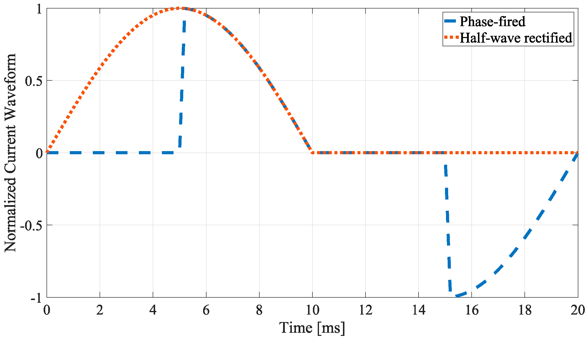
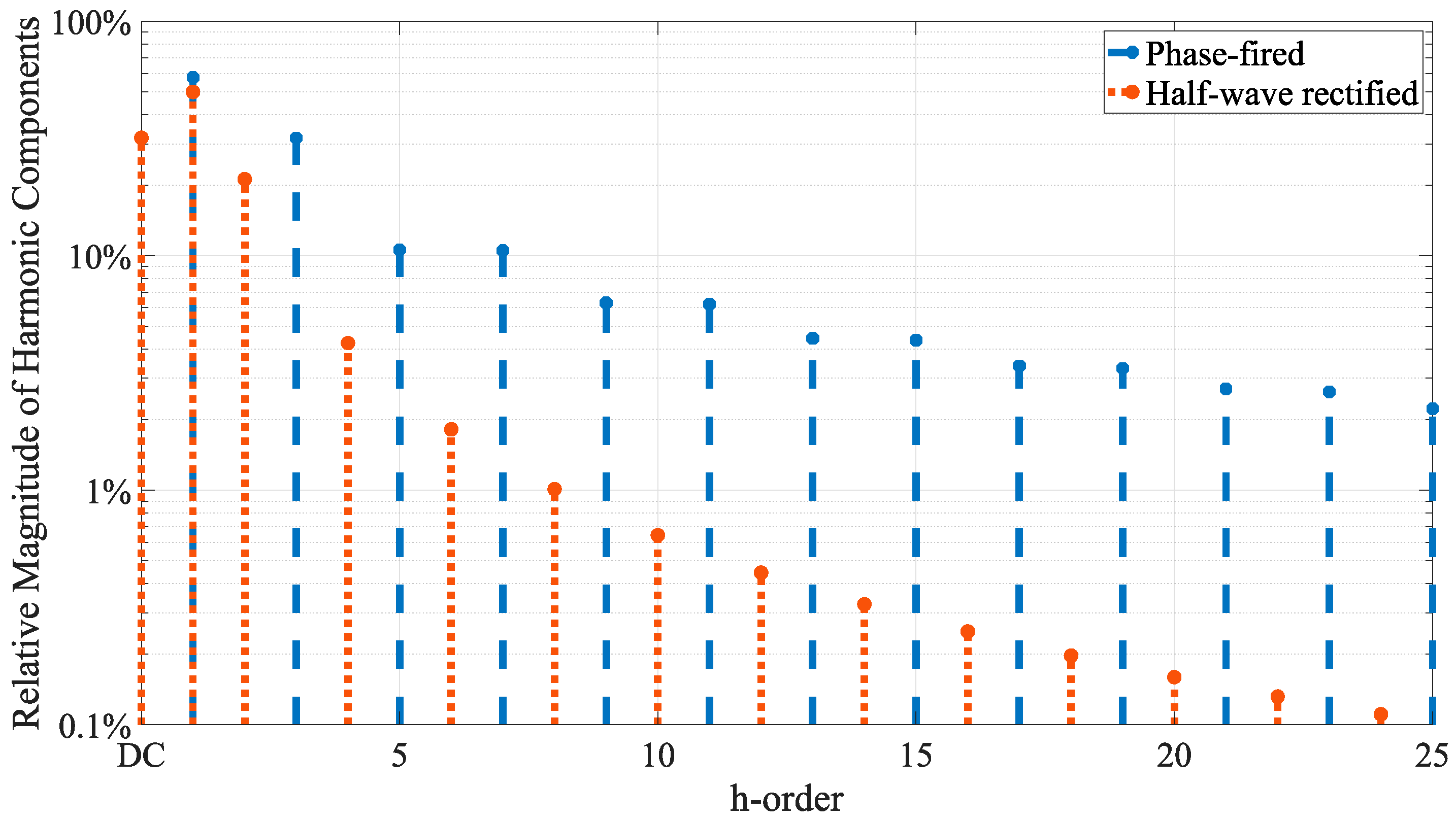
The peculiarity of all the harmonic disturbance tests for the active EMs calibration is the fact that a standard test waveform has been chosen, distinguished by a very specific harmonic content. For instance, in the disturbance category (i) the voltage and current waveforms are both formed by a fundamental and a 5th harmonic component, but with different Total Harmonic Distortion factor (THD): 10% for the voltage and 40% for the current. The fundamental and the 5th component of voltage are in phase at the positive zero crossing and the current components are in phase with the same-order voltage components. As for the disturbance category (ii), the standards establish a half-wave rectified current waveform, composed just by even harmonics with a THD $\approx 87\%$, while for the disturbance category (iii), a phase-fired alternate current waveform, made by odd harmonics and characterized by a THD $\approx 113\%$ is defined. In Figure 1 and Figure 2 the time-domain signal and the magnitude spectrum of the mentioned test waveforms are depicted, respectively.

3. Measurement System Description

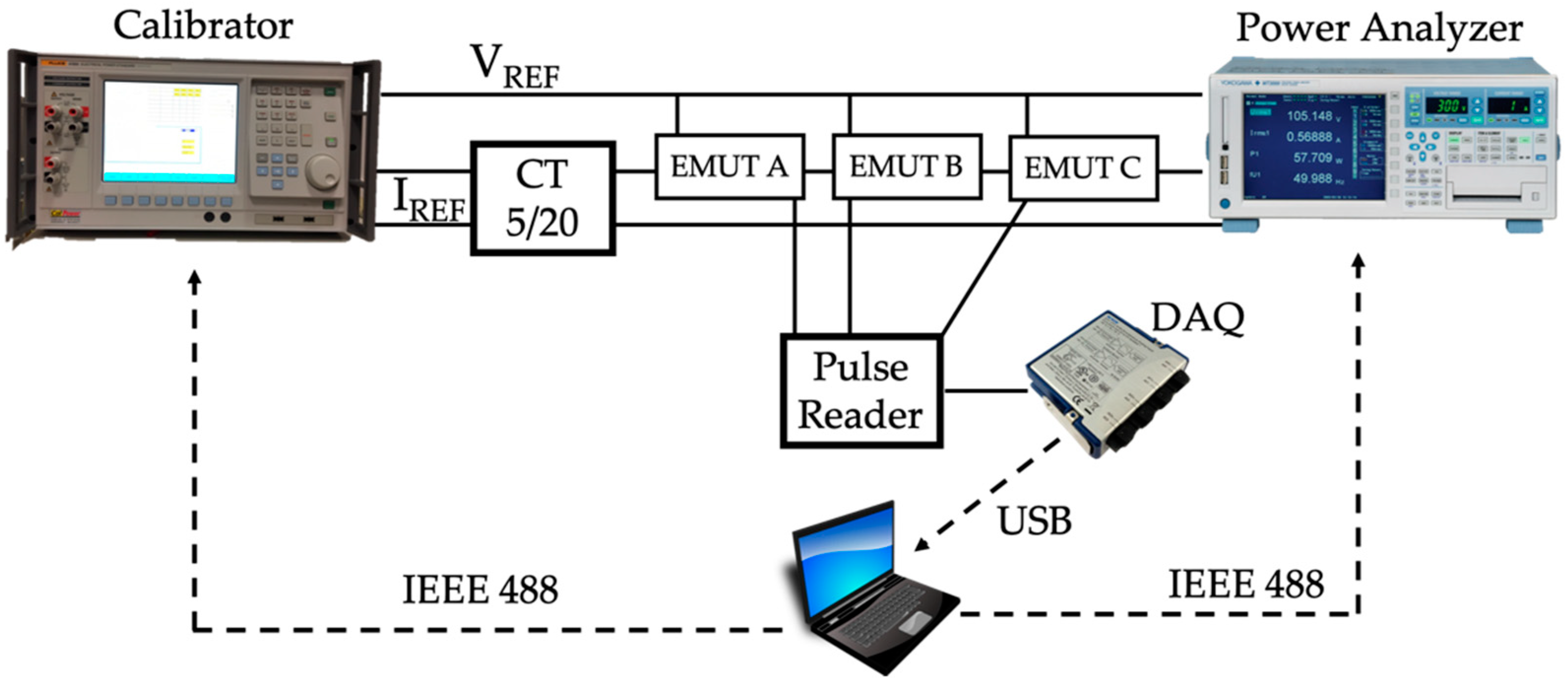
The experimental tests were carried out by means of the test setup illustrated in Figure 3, analogous to the one presented in [32], except for an additional energy meter under test (EMUT) connected in series to the current circuit and in parallel to the voltage one.

Since full information concerning the test setup can be found in [32], in the following just a brief summary of the employed equipment is reported and the specifications of the new EMUT are listed. A Fluke 6105A calibrator provided the reference voltage and current inputs. The voltage is directly applied across the EMUTs terminals, while the current is stepped-up by means of a 5 VA 5:20 current transformer (CT), feeding the EMUTs. A high-accuracy power analyzer Yokogawa WT3000E, of which accuracy is ± (0.01% of reading + 0.03% of range + 0.02% of time reading), served as reference for the active energy measurement. The three EMUTs, identified as EMUT A, B, and C, are single-phase MID class B compliant, according to the standard EN 50470-3. In spite of the same rated voltage $U_n=$ 230 V and the same rated current $I_{\mathit{ref}}$ = 5 A, the EMUT C maximum current $I_{\mathit{max}}$ is 100 A ($I_{\mathit{max}}$ = 45 A for EMUT A, $I_{\mathit{max}}$ = 40 A for EMUT B) and it is equipped with a static pulsed test output at 1000 impulses per unit of energy (imp/kWh). The three test outputs have been connected to a pulse reader, made of three signal conditioning circuits based on a photodetector (for EMUT A) and two pull-up resistors (one for EMUT B and one for the EMUT C), cascaded with logical ports acting as voltage regulators to obtain 0–5 V at the output. These three signals at the output have been acquired through a NI9239 24-bit Data Acquisition board (DAQ) connected to a host PC running the test automation.

4. Experimental Tests

The tests proposed in this paper are aimed at evaluating the EMs behavior when the voltage and the current are not sinusoidal. It should be highlighted that they are not only distorted waveforms, but they are also distinguished by a realistic harmonic content for an LV distribution network, considering the limits defined in the standards [29,30]. Three different tests were carried out, all of them are based on the setup sketched in Figure 3:

• sinusoidal waveform test (calibration measurement);
• fixed random harmonics test;
• random time-varying harmonics test.

In these three tests, detailed in the following, the calibrator generated a sinusoidal current and voltage at $f_r=50\mathrm{Hz}$. Only in the last two tests, an additional harmonic content up to the 25th harmonic was superimposed to the 50 Hz components. The relative phase displacement between voltage and current was set equal to zero for all the frequency components (pure resistive load), to focus only on the effect of the harmonic content on the active energy measurements performed by the EMs. This scenario is meaningful since the loads’ power factor is very close to 1 in typical LV power networks. The current from the calibrator $I_p$ has been stepped-up to $I_s$ by a factor of 4 through the CT and then fed to the EMUTs. The potential of the secondary winding of the CT has been raised to U in order to obtain a phantom power supply for the EMUTs. The active energies $E_{\mathit{mA}}$, $E_{\mathit{mB}}$, and $E_{\mathit{mC}}$ measured by EMUT A, EMUT B, and EMUT C, respectively, are compared against $E_t$, the energy measured by the reference power analyzer. The synchronization of the readings from the EMUTs and the power analyzer was implemented by starting the pulse counter acquisition in parallel with the energy computation performed by the power analyzer. The active energy readings were triggered when the electrical quantities provided by the calibrator were already in steady state. A detailed analysis on the “pulse reader + DAQ” system properties is conducted in the Appendix A section.

4.1. Sinusoidal Current And Voltage-Calibration Measurement

The first test consisted of providing a sinusoidal current ($I_p=5\mathrm{A}$, rms) and a sinusoidal voltage ($U=230\mathrm{V}$, rms) by means of the Fluke 6105A to carry out the calibration of the EMUT C at nominal conditions and to check its measurement repeatability. Note that this operation had been already performed for EMUTs A and B in [32]. The time duration of this calibration test is about 8 h in order to replicate the same conditions under which EMUT A and B were subjected to. Note also that such a long-duration test makes negligible the contribution to uncertainty due to the test output reading compared to the overall energy measured by the EMUT. The chosen value for $I_s$ is 20 A since it lays between $I_{\mathit{ref}}$ and $I_{\mathit{max}}$ for all the three EMUTs and also because it is representative of a typical current intensity at the node where the EMs are installed in residential applications. This calibration procedure was repeated 8 times. For each repetition, the calibration coefficient $K_{\mathit{EM}C}$ was computed as:

$$K_{\mathit{EM}C}=\frac{E_{\mathit{mC}}}{E_t}$$

(3)

where $E_{\mathit{mC}}$ is the active energy reading from EMUT C and $E_t$ is the corresponding reading of the reference instrument. Afterwards, the computations of the mean value ${\overline{K}}_{\mathit{EM}C}$ and of the standard deviation of the mean ${\sigma }_{K_{\mathit{EM}}C}$ were carried out by evaluating the 8 values obtained by each test repetition.

The coefficient ${\overline{K}}_{\mathit{EM}C}$ and the ones computed in [32], ${\overline{K}}_{\mathit{EM}A}$ and ${\overline{K}}_{\mathit{EM}B}$, for EMUT A and B, respectively, have been then used to correct the $E_m$ in all the following tests (see Section 4.2 and Section 4.3). The correction is performed through:

$${E*}_{mi}=\frac{E_{mi}}{{\overline{K}}_{\mathit{EM}i}}$$

(4)

where: i = A, B and C; ${E*}_{mi}$ is the EMUT i’s corrected active energy reading. This procedure allows assessing the effect of the considered harmonic disturbances by means of the additional percentage error $e_i^{*}\%$:

$$e_i^{*}\%=\frac{{E*}_{mi}-E_t}{E_t}\cdot 100$$

(5)

4.2. Fixed Random Harmonics

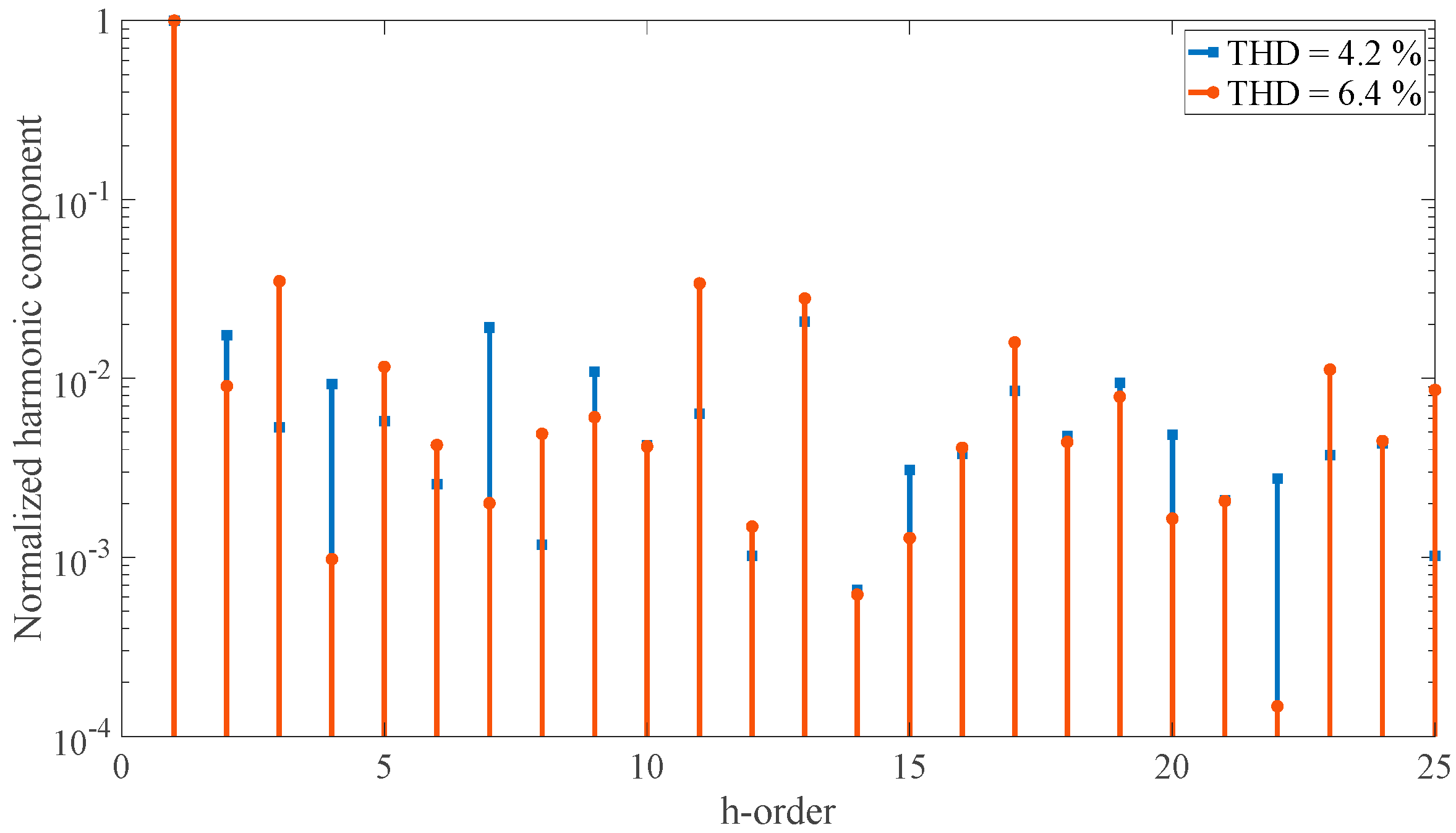
In the second test, two sets of current and voltage harmonics were randomly generated, complying with the limits prescribed by [30] for the voltage harmonics up to the 25th order in LV systems. Each voltage harmonic component was drafted from a uniform distribution that ranges from 0 to the corresponding limit presented in the EN 50,160 standard. Since a pure resistive load was assumed, as mentioned above, the current harmonic relative amplitudes were analogous to the voltage ones and the overall rms value was set to $I_p=5\mathrm{A}.$ The THD of the waveforms obtained according to the described procedure were 4.2% and 6.4%, which are realistic values for current and voltage distortion according to those highlighted in the standard [29]. The experiment based on the test waveform with THD = 4.2% will be addressed as ♮1, while the one based on the test waveform with THD = 6.4% as ♮2. The magnitude spectra of the waveforms are represented in Figure 4 and are normalized to the 50 Hz component magnitude. The time duration of this test is about 8 h. Finally, the effects of the fixed random harmonic are evaluated by applying Equations (4) and (5).

4.3. Random Time-Varying Harmonic Distorsion

The third test’s objective is to simulate a realistic scenario in which the energy meters are subjected to a harmonic distortion that changes unpredictably over time. To achieve this, a distorted voltage and current waveforms both generated with the same technique, illustrated in Section 4.2, were applied for a short time interval (about 10 min). After that, another random waveform was applied, and so on for about 8.5 h. This operation was repeated 7 times. Finally, the effects of the random time-varying harmonic distortions are evaluated by applying Equations (4) and (5).

5. Experimental Results

5.1. Sinusoidal Current And Voltage-Calibration Measurement

In

Table 4. EMUT C calibration at nominal sinusoidal conditions.

	${\mathit{E}}_{\mathit{t}}\left(\mathbf{Wh}\right)$	${\mathit{E}}_{\mathit{mC}}\left(\mathbf{Wh}\right)$	${\mathit{K}}_{\mathit{EM}\mathit{C}}$	${\mathit{e}}_{\mathit{C}}\%(\%)$
	36,416.0	36,648	1.00637	0.64
	36,419.5	36,658	1.00655	0.65
	36,420.8	36,660	1.00657	0.66
	36,423.7	36,663	1.00657	0.66
	36,407.3	36,657	1.00686	0.69
	36,404.6	36,658	1.00696	0.70
	36,406.7	36,662	1.00701	0.70
	36,406.9	36,662	1.00701	0.70
${\overline{K}}_{\mathit{EM}}$			1.00674
${\sigma }_{K_{\mathit{EM}}}$			9 × 10−5

, the data from the EMUT C calibration is reported, whereas the summary of the EMUTs’ A and B results obtained in [32] are listed in

Table 5. EMUTs A and B calibration at nominal sinusoidal conditions.

	EMUT A	EMUT B
	0.9983	1.00892
${\sigma }_{K_{\mathit{EM}}}$a	2 × 10−5	4 × 10−5

^a The corresponding samples are shown in [32].

. The percentage error $e_C\%$ has been computed according to Equation (1) and $K_{\mathit{EM}C}$ according to Equation (3). Note that, even for EMUT C, the standard deviation ${\sigma }_{K_{EM C}}$, associated to the computed average calibration coefficient, is very limited compared to the related average value ${\overline{K}}_{\mathit{EM}C}$ and consistent with the ones obtained for EMUT A and EMUT B in [32] and reported in Table 5 for the sake of readability. This result means that the EMUT A, EMUT B, and EMUT C calibration measurements are distinguished by a good repeatability (all obtained standard deviations are at least 5000 times lower than the measured quantity). Finally, a check of the accuracy class has been conducted, and since the percentage error is about 0.70%, the EMUT C has been proved to be widely compliant with the declared class (as for the EMUTs A and B).

5.2. Fixed Random Harmonics

In

Table 6. EMUTs additional percentage error at random distorted current and voltage condition.

	THD (%)	${\mathit{E}}_{\mathit{t}}\left(\mathbf{Wh}\right)$	${\mathit{E}*}_{\mathit{mA}}\left(\mathbf{Wh}\right)$	${\mathit{E}*}_{\mathit{mB}}\left(\mathbf{Wh}\right)$	${\mathit{E}*}_{\mathit{mC}}\left(\mathbf{Wh}\right)$	${\mathit{e}}_{\mathit{A}}^{*}\%(\%)$	${\mathit{e}}_{\mathit{B}}^{*}\%(\%)$	${\mathit{e}}_{\mathit{C}}^{*}\%(\%)$
♮1	4.2	36,529.1	36,528.3	36,474.8	36,514.0	0.00	−0.15	−0.04
♮2	6.4	36,532.2	36,539.2	36,474.8	36,512.0	0.02	−0.16	−0.06

, the readings and the additional percentage errors $e_i^{*}\%$ (i = A, B, and C) regarding the active energy measurements for the two fixed random harmonics tests are collected. The standard uncertainty $u_{\mathit{ei}\%}$ of each additional percentage error computed for this test is shown in the top row of

Table 7. Evaluation of Standard Uncertainty for the EMUTs additional percentage errors.

		${\mathit{u}}_{\mathit{eA}\%}(\%)$	${\mathit{u}}_{\mathit{eB}\%}(\%)$	${\mathit{u}}_{\mathit{eC}\%}(\%)$
Fixed random harmonics	♮1	0.09	0.09	0.09
	♮2
Random time-varying harmonics	#1	0.2	0.2	0.2
	#2
	#3
	#4
	#5
	#6
	#7

.

Examining also the $e_i^{*}\%$ values in Table 6, it can be noticed that: first, the magnitude of EMUT B’s percentage error is greater than $u_{\mathit{eB}\%}$ by around 2 times; second, the values of $e_A^{*}\%$ and $e_C^{*}\%$ are of the same order of magnitude of (and even smaller than) $u_{\mathit{eA}\%}$ and $u_{\mathit{eC}\%}$. Given that, the analysis of the presented values is carried out according to the following considerations. Thanks to the average calibration coefficient ${\overline{K}}_{\mathit{EM}C}$ definition, it is possible to express the additional percentage error $e_i^{*}\%$ (I = A, B, C) by Equation (5). $e_i^{*}\%$ is equal to zero (within the limits of the variation associated with ${\overline{K}}_{\mathit{EM}C}$) if ${E*}_{mi}$ (I = A, B, C) is measured in conditions analogous to the ones of the calibration procedure. When the current and voltage distortion is introduced, the root mean square (RMS) values are the same as the ones related to the sinusoidal quantities used for the calibration. The reference energy meter is assumed to not present a significantly different behavior in the distorted conditions, given its wide bandwidth. Therefore, any value of the $e_i^{*}\%$ different from zero observed in distorted conditions may be attributed to a performance downgrade of the EMs in these conditions. But first, the uncertainty associated to $e_i^{*}\%$ must be considered: if its confidence interval does not include zero, then it is reasonable to state that the EMs’ behavior have been affected by the introduced distortion; otherwise, if the interval includes zero, the impact of the distortion is not observable and nothing can be stated. Finally, the confidence interval has been computed as a double-sided interval centered in $e_i^{*}\%$ by means of the standard uncertainty.

According to the analysis above, only EMUT B shows a slight influence due to the fixed random harmonic presence, given that the relative confidence intervals are [−0.24%, −0.06%] and [−0.25%, −0.07%].

5.3. Random Time-Varying Harmonic Distorsion

In

Table 8. THD range maximum and minimum values with random time-varying harmonic distorted current and voltage distortion.

Sequence	THD Min (%)	THD Max (%)
#1	3.5	6.9
#2	3.5	6.9
#3	3.8	7.0
#4	3.8	7.0
#5	3.2	6.9
#6	4.2	7.0
#7	3.7	7.5

, there are listed the observed maximum and minimum THD values of the generated current and voltage waveforms for each test sequence.

For each sequence, the ${E*}_{\mathrm{mi}}$ values, the reference energy readings $E_t$ and the $e_i^{*}\%$ are shown in

Table 9. EMUTs additional percentage error with random time-varying harmonic distorted current and voltage distortion.

Sequence	${\mathit{E}}_{\mathit{t}}\left(\mathbf{Wh}\right)$	${\mathit{E}*}_{\mathit{mA}}\left(\mathbf{Wh}\right)$	${\mathit{E}*}_{\mathit{mB}}\left(\mathbf{Wh}\right)$	${\mathit{E}*}_{\mathit{mC}}\left(\mathbf{Wh}\right)$	${\mathit{e}}_{\mathit{A}}^{*}\%(\%)$	${\mathit{e}}_{\mathit{B}}^{*}\%(\%)$	${\mathit{e}}_{\mathit{C}}^{*}\%(\%)$
#1	38,075.1	38,201.9	38,060.6	38,075.5	0.3	0.0	0.0
#2	38,067.3	38,194.0	38,060.6	38,078.5	0.3	0.0	0.0
#3	38,059.4	38,192.0	38,060.6	38,067.5	0.3	0.0	0.0
#4	38,061.8	38,177.2	38,060.6	38,082.4	0.3	0.0	0.1
#5	38,053.8	38,167.3	38,060.6	38,068.5	0.3	0.0	0.0
#6	38,050.9	38,160.4	38,060.6	38,072.5	0.3	0.0	0.0
#7	38,051.4	38,107.9	38,060.6	38,079.5	0.1	0.0	0.0

, while the standard uncertainties $u_{\mathit{ei}\%}$ of the additional percentage errors $e_i^{*}\%$ are reported in the bottom row of Table 7.

The random current and voltage distortion variations lead to percentage error variations that are not significative for EMUT B and C: as a matter of fact, the $u_{\mathit{ei}\%}$ values define confidence intervals including zero (see observations in Section 4.2). On the contrary, EMUT A exhibits a [0.1%, 0.5%] confidence interval of $e_i^{*}\%$ for the sequences #1 to #6. Then, it can be concluded that the effect of the test scenario where the harmonic distortion of the current and the voltage waveforms randomly evolves over the time is not negligible for the EMUT A. Finally, observing Table 7, one could question the fact that the uncertainties relative to the percentage errors in the random time-varying harmonic test are higher than the ones in the fixed random harmonic test. This results from the test setup. In order to change the harmonic content of the voltage and current waveforms, the calibrator outputs must be set on standby and the active energy cannot be measured during the transients between the standby and operational states because they would pollute the measurement. Therefore, considering that each harmonic configuration shall be applied for about 10 min, the present test results in performing about 50 different measurements and then to sum the readings of each measurement. Hence, the uncertainty of the $e_i^{*}\%$ relative to the cumulative readings is higher than the uncertainty obtained in the fixed random harmonic cases. However, even if this uncertainty is twice the one in the fixed random harmonics case, it is still possible to observe whether the EMUTs’ behavior is affected. Of course, the variation of the measured quantity must be evaluated against its confidence interval in order to judge the experimental result.

6. Conclusions

The energy meter performances are affected by the spread of new actors among the grid, which degrade the overall power quality and the quantities to be measured. This challenging scenario and the need of more and more network observability demand new testing procedures to be developed.

To this purpose, three off-the-shelf energy meters have been tested by applying distorted current and voltage waveforms. Their behavior has been assessed computing the index prescribed by the standards to verify whether distorted conditions affect the energy meters accuracy. From the results it is possible to conclude that (i) the adopted waveforms and the measurement setup implemented allow appreciating small variations in the energy meters accuracy; (ii) not all the energy meters are affected by distorted conditions. Therefore, considering the test waveforms prescribed by the standards and the results herein presented, it can be concluded that the standards should improve in terms of incorporating more realistic test waveforms to better assess the energy meters’ behavior in realistic conditions.

References

1. Qianjun, Y.; Guichu, W.; Fenqun, Y.; Hongyan, X. Design and applications of intelligent low voltage distribution system based on ZigBee. In Proceedings of the International Conference on Electronics, Communications and Control, Ningbo, China, 9–11 September 2011. [Google Scholar]
2. Löf, A.; Repo, S.; Pikkarainen, M.; Lu, S.; Pöhö, T. Low voltage network monitoring in RTDS environment. In Proceedings of the IEEE PES ISGT Europe, Lyngby, Denmark, 12–15 October 2013. [Google Scholar]
3. Lu, S.; Repo, S.; Della Giustina, D.; Figuerola, F.A.C.; Löf, A.; Pikkarainen, M. Real-Time Low Voltage Network Monitoring—ICT Architecture and Field Test Experience. IEEE Trans. Smart Grid 2015, 6, 2002–2012. [Google Scholar] [CrossRef]
4. Mingotti, A.; Ghaderi, A.; Mazzanti, G.; Peretto, L.; Tinarelli, R.; Valtorta, G.; Danesi, S. Low-cost monitoring unit for MV cable joints diagnostics. In Proceedings of the 9th IEEE International Workshop on Applied Measurements for Power Systems (AMPS 2018), Bologna, Italy, 26–28 September 2018. [Google Scholar]
5. Mingotti, A.; Ghaderi, A.; Peretto, L.; Tinarelli, R.; Lama, F. Test setup design, and calibration for tan delta measurements on MV cable joints. In Proceedings of the 9th IEEE International Workshop on Applied Measurements for Power Systems (AMPS), Bologna, Italy, 26–28 September 2018. [Google Scholar]
6. Farhangi, H. The path of the smart grid. IEEE Power Energy Mag. 2010, 8, 18–28. [Google Scholar] [CrossRef]
7. Sanchez, R.; Iov, F.; Kemal, M.; Stefan, M.; Olsen, R. Observability of low voltage grids: Actual DSOs challenges and research questions. In Proceedings of the 52nd International Universities Power Engineering Conference (UPEC), Heraklion, Greece, 28–31 August 2017. [Google Scholar]
8. Al-Wakeel, A.; Wu, J.; Jenkins, N. State estimation of medium voltage distribution networks using smart meter measurements. Appl. Energy 2016, 184, 207–218. [Google Scholar] [CrossRef] [Green Version]
9. Mingotti, A.; Peretto, L.; Tinarelli, R. A Novel Equivalent Power Network Impedance Approach for Assessing the Time Reference in Asynchronous Measurements. In Proceedings of the 2017 IEEE International Instrumentation and Measurement Technology Conference, I2MTC, Torino, Italy, 22–25 May 2017; pp. 624–629. [Google Scholar]
10. Nasrollahi, S.; Sardarabadi, A.; Khoshian, Y.; Gharib, A. A novel hybrid algorithm for reconfiguration problem of the distribution networks. In Proceedings of the 22nd International Conference and Exhibition on Electricity Distribution, Stockholm, Sweden, 10–13 June 2013. [Google Scholar]
11. Liu, Y.; Wang, Z.; Meng, X.; Sheng, W. Distribution network planning considering distributed generations based on genetic algorithm. In Proceedings of the IEEE Power Engineering and Automation Conference, Wuhan, China, 8–9 September 2011. [Google Scholar]
12. Zhang, J.; Huang, T.; Zhang, H. The Reactive Power Optimization of Distribution Network Based on an Improved Genetic Algorithm. In Proceedings of the IEEE/PES Transmission Distribution Conference Exposition: Asia and Pacific, Dalian, China, 18 August 2005. [Google Scholar]
13. Ferrero, A.; Faifer, M.; Salicone, S. On Testing the Electronic Revenue Energy Meters. IEEE Trans. Instrum. Meas. 2009, 58, 3042–3049. [Google Scholar] [CrossRef] [Green Version]
14. Sun, Q.; Li, H.; Ma, Z.; Wang, C.; Campillo, J.; Zhang, Q.; Wallin, F.; Guo, J. A Comprehensive Review of Smart Energy Meters in Intelligent Energy Networks. IEEE Internet Things J. 2016, 3, 464–479. [Google Scholar] [CrossRef]
15. Cetina, R.Q.; Roscoe, A.J.; Wright, P.S. A review of electrical metering accuracy standards in the context of dynamic power quality conditions of the grid. In Proceedings of the 2017 52nd International Universities Power Engineering Conference (UPEC), Heraklion, Greece, 28–31 August 2017. [Google Scholar]
16. Ferrero, A.; Peretto, L.; Sasdelli, R. Revenue metering in the presence of distortion and unbalance: Myths and reality. In Proceedings of the 8th International Conference on Harmonics and Quality of Power, (Cat. No.98EX227), Athens, Greece, 14–16 October 1998; pp. 42–47. [Google Scholar]
17. Bernieri, A.; Betta, G.; Ferrigno, L.; Laracca, M. Electrical energy metering in compliance with recent european standards. In Proceedings of the 2012 IEEE International Instrumentation and Measurement Technology Conference Proceedings, Graz, Austria, 13–16 May 2012; pp. 1541–1545. [Google Scholar]
18. Novotny, J.; Drapela, J.; Topolanek, D. Frequency response of revenue meters in measured active energy. In Proceedings of the 2016 17th International Conference on Harmonics and Quality of Power (ICHQP), Belo Horizonte, Brazil, 16–19 October 2016; pp. 524–529. [Google Scholar]
19. Femine, A.D.; Gallo, D.; Landi, C.; Luiso, M. Advanced Instrument for Field Calibration of Electrical Energy Meters. IEEE Trans. Instrum. Meas. 2009, 58, 618–625. [Google Scholar] [CrossRef]
20. Cataliotti, A.; Cosentino, V.; Nuccio, S. Static Meters for the Reactive Energy in the Presence of Harmonics: An Experimental Metrological Characterization. IEEE Trans. Instrum. Meas. 2009, 58, 2574–2579. [Google Scholar] [CrossRef]
21. Cataliotti, A.; Cosentino, V.; Lipari, A.; Nuccio, S. Metrological Characterization and Operating Principle Identification of Static Meters for Reactive Energy: An Experimental Approach Under Nonsinusoidal Test Conditions. IEEE Trans. Instrum. Meas. 2009, 58, 1427–1435. [Google Scholar] [CrossRef]
22. Gallo, D.; Landi, C.; Pasquino, N.; Polese, N. A New Methodological Approach to Quality Assurance of Energy Meters under Nonsinusoidal Conditions. IEEE Trans. Instrum. Meas. 2007, 56, 1694–1702. [Google Scholar] [CrossRef]
23. Georgakopoulos, D.; Wright, P.S. Calibration of energy and power meters under non-sinusoidal conditions. IEE Proc. Sci. Meas. Technol. 2006, 153, 241–247. [Google Scholar] [CrossRef] [Green Version]
24. Mingotti, A.; Peretto, L.; Tinarelli, R.; Zhang, J. Use of COMTRADE Fault Current Data to Test Inductive Current Transformers. In Proceedings of the IEEE Workshop on Metrology for Industry 4.0 and IoT, Naples, Italy, 4–6 June 2019. [Google Scholar]
25. Rietveld, G.; Sloot, W.; So, E.; Guo, X.; Mubarak, F.; de Geus, J.; van Halm, F.; Wismans, B.; Bruijns, S.; Koers, F.; et al. Performance evaluation of HV CTs subjected to actual operating conditions in substations and its impact on smart metering infrastructure within smart grids. In Proceedings of the IEEE Power and Energy Society General Meeting, San Diego, CA, USA, 22–26 July 2012. [Google Scholar]
26. So, E.; Arseneau, R.; Bennett, D.; Frigault, M. A current-comparator-based system for calibrating high voltage conventional and non-conventional current transformers under actual operating conditions of high voltage and distorted current waveforms up to 100 kV and 2000 A. In Proceedings of the CPEM 2010 Daejeon, South Korea, 13–18 June 2010. [Google Scholar]
27. Mahesh, G.; George, B.; Jayashankar, V.; Kumar, V.J. Instrument transformer performance under distorted-conditions. In Proceedings of the IEEE INDICON 2004 First India Annual Conference, Kharagpur, India, 20–22 December 2004. [Google Scholar]
28. Lei, T.; Cristaldi, L.; Faifer, M.; Ottoboni, R.; Toscani, S.; Cherbaucich, C.; Mazza, P. Behavior of voltage transformers under distorted conditions. In Proceedings of the International Instrumentation and Measurement Technology Conference, Taipei, Taiwan, 23–26 May 2016. [Google Scholar]
29. IEEE Std 519-2014, Recommended Practice and Requirements for Harmonic Control in Electric Power Systems; IEEE: New York, NY, USA, 2014.
30. EN 50160:2011, Voltage Characteristics of Electricity Supplied by Public Electricity Networks; European Committee for Standardization: Brussels, Belgium, 2017.
31. Dichiarazione di Conformità Alla Direttiva 2014/53/UE “RED”, e-Distribuzione S.p.A. 2017. Available online: https://www.e-distribuzione.it/content/dam/e-distribuzione/documenti/open-meter/dichiarazione_conformit%C3%A0/Dichiarazione_conformit%C3%A0_Direttiva_Europa2014_53_UE_Direttiva_RED.pdf (accessed on 7 June 2019).
32. Bartolomei, L.; Cavaliere, D.; Mingotti, A.; Peretto, L.; Tinarelli, R. Testing of Electrical Energy Meters in Off-Nominal Frequency Conditions. In Proceedings of the 2019 IEEE 10th International Workshop on Applied Measurements for Power Systems (AMPS), Aachen, Germany, 25–27 September 2019. [Google Scholar]
33. European Parliament and of the Council. EU Directive on Measuring Instruments (MID); 2014/32/EU; European Parliament and of the Council: Brussels, Belgium, 2014. [Google Scholar]
34. CENELEC. Electricity Metering Equipment (A.C.)—Part 1: General Requirements, Tests and Test Conditions—Metering Equipment (Class Indexes A, B and C); EN 50470-1:2006+A1:2018; CENELEC: Brussels, Belgium, 2018. [Google Scholar]
35. CENELEC. Electricity Metering Equipment (A.C.)—Part 2: Particular Requirements—Electromechanical Meters for Active Energy (Class Indexes A and B); EN 50470-2:2006+A1:2018; CENELEC: Brussels, Belgium, 2018. [Google Scholar]
36. CENELEC. Electricity Metering Equipment (A.C.)—Part 3: Particular Requirements—Static Meters for Active Energy (Class Indexes A, B and C); EN 50470-3:2006+A1:2018; CENELEC: Brussels, Belgium, 2018. [Google Scholar]
37. IEC. Electricity Metering Equipment (A.C.)—General Requirements, Tests and Test Conditions—Part 11: Metering Equipment; IEC 62052-11:2003+A1:2016; IEC: Geneva, Switzerland, 2016. [Google Scholar]
38. IEC. Electricity Metering Equipment (A.C.)—Particular Requirements—Part 21: Static Meters for Active Energy (Class 1 and 2); IEC 62053-21:2003/A1:2016; IEC: Geneva, Switzerland, 2016. [Google Scholar]
39. IEC. Electricity Metering Equipment (A.C.)—Particular Requirements—Part 21: Static Meters for Active Energy (Class 0, 2S and 0, 5S); IEC 62053-22:2003+A1:2016; IEC: Geneva, Switzerland, 2016. [Google Scholar]
40. IEC. Electricity Metering Equipment (A.C.)—Particular Requirements—Part 31: Pulse output Devices for Electromechanical and Electronic Meters (Two Wires only); IEC 62053-31:1998; IEC: Geneva, Switzerland, 1998. [Google Scholar]
Figure 1. Odd and even harmonic disturbance tests waveforms defined in EN 50470-3 and IEC 62053-21.
Energies 13 02023 g001
Figure 2. Odd and even harmonic disturbance tests waveforms magnitude spectra defined in EN 50470-3 and IEC 62053-21.
Energies 13 02023 g002
Figure 3. Adopted measurement setup for testing the 3 off-the-shelf energy meters (Ems).
Energies 13 02023 g003
Figure 4. Normalized harmonic components randomly generated for the “Fixed random harmonics” tests ♮1 (THD = 4.2%) and test ♮2 (THD = 6.4%). THD, Total Harmonic Distortion.
Energies 13 02023 g004