Abstract
Given the imminent threats of climate change, it is urgent to boost the use of clean energy, being wind energy a potential candidate. Nowadays, deployment of wind turbines has become extremely important and long-term estimation of the produced power entails a challenge to achieve good prediction accuracy for site assessment, economic feasibility analysis, farm dispatch, and system operation. We present a method for long-term wind power forecasting using wind turbine properties, statistics, and genetic programming. First, due to the high degree of intermittency of wind speed, we characterize it with Weibull probability distributions and consider wind speed data of time intervals corresponding to prediction horizons of 30, 25, 20, 15 and 10 days ahead. Second, we perform the prediction of a wind speed distribution with genetic programming using the parameters of the Weibull distribution and other relevant meteorological variables. Third, the estimation of wind power is obtained by integrating the forecasted wind velocity distribution into the wind turbine power curve. To demonstrate the feasibility of the proposed method, we present a case study for a location in Mexico with low wind speeds. Estimation results are promising when compared against real data, as shown by MAE and MAPE forecasting metrics.
1. Introduction
To achieve the maximum use of wind energy, the prediction of the wind resource is mandatory since it is one of the main ingredients to estimate the generated wind power by a wind turbine generator or a wind power plant. Time scales for wind forecasting can be divided into four categories according to the literature [1]:
- Very short-term forecast: From a few minutes to one hour ahead.
- Short-term forecast: From one hour to several hours ahead.
- Medium-term forecast: From several hours to one week ahead.
- Long-term forecast: From one week to one year or more ahead.
The usefulness of the prediction depends on the prediction horizon. For instance, very short forecasting is important for the electricity market clearing and real-time grid operation. Short-term wind predictions are relevant for load dispatch planning, load decision, feedback voltage and power control, protection to preserve physical integrity and operational security in the electricity market. Medium-term wind prediction is useful for economic dispatch, unit commitment decision, electricity market and maintenance. Finally, long-term wind prediction is convenient for dispatch planning, system planning, financial investments, operation management, optimal operation cost and feasibility analysis of the wind farm [2,3]. In this work, we develop a methodology for long-term wind power forecasting.
Wind power forecasting is made either by deterministic or probabilistic prediction. The first approach considers the topographical and meteorological properties of the site to predict the wind field and thereafter the energy potential. On the other hand, the statistical approach mainly uses probability distributions that relate variables with wind power to perform predictions [4].
The most typical probability distribution functions to describe wind statistics are the Rayleigh and Weibull distributions [5]. By considering the wind velocity vector and assuming that each orthogonal component is uncorrelated and normally distributed, the magnitude of the velocity vector is characterized by a Rayleigh distribution [6,7]. On the other hand, the Weibull distribution, which interpolates between the exponential distribution and the Rayleigh distribution provides a better fit to the probability density distribution of the wind speed [8]. The Weibull distribution is typically used for assessment of wind energy potentials, in particular, it is used in reliability and maintainability analysis, selection of location for wind turbine generators and performance of wind farms. There are several reported works on the use of Weibull distribution to analyze the wind resource. In 2010, Bhattacharya [9] presented analytical and computational methods for the estimation of Weibull parameters for wind velocity distributions. In 2013, Giebel et al. [10] analyzed two models for wind speed prediction: (a) a structural stochastic model to predict wind speeds exponentially using a linear combination of separate mean-reverting jump processes for the high and low wind speeds; and (b) a neuro-stochastic model to predict the wind velocity with parameters updating dynamically from a re-weighted history. In 2014, Azad et al. [11] studied the Weibull distribution of the wind resource of Hatiya Island in Bangladesh, finding an average wind speed of 6 m/s and concluding that the site has good power to drive small wind turbines for electricity generation. In 2015, Yenilmez et al. [12] introduced a modified Weibull distribution for modeling wind speed and estimating wind power density. In the same year, Azad et al. [13] presented three different statistical tools for estimating the Weibull distribution in Bangladesh to identify prospects for windy sites.
Regarding forecasting, the probabilistic approach provides an estimation of the probabilities for the possible future outcomes of a random variable. At its best, a probabilistic forecast provides a probability density function that describes the possible behavior of a random variable for a coming event or time horizon [14]. Probabilistic forecast has been playing a major role in weather forecasting [15], sports betting [16], macroeconomic forecasting [17] and population forecasting [18]. It is believed that probabilistic forecasting can also play a major role in energy forecasting, as motivated by the Global Energy Forecasting Competition 2014 aimed at probabilistic forecasting of electric load, wind and solar power and electricity prices [19]. Specifically, probabilistic forecast seems to be well suited for clean electric power production from renewable energies because of the random nature of the primary energy supply, mainly wind and solar irradiation. Zhou et al. [20] used probabilistic wind power forecasting in electricity markets for scheduling and dispatch purposes. They forecasted the probability density function using probabilistic kernel density forecasting with a quantile estimator. Wan et al. [21] developed a methodology for wind power forecasting in a nonparametric probabilistic approach using direct quantile regression and machine learning. They produced quantiles with linear programming and multistep probabilistic forecasting of 10-min wind power data with real wind farm data. Xydas et al. introduced a methodology to define wind power forecast scenarios using historical wind power time series data and Kernel probability densities [22]. The forecast scenarios are inputs for unit commitment and optimal dispatch model to investigate the way wind forecast uncertainty affects the operation of the power system.
Genetic Programming (GP) is a heuristic search technique developed to evolve a population of computer programs that solve a given problem into a new generation of programs that solve the problem more effectively by using genetic operations [23]. The GP process comprehends the following steps: evaluation of program fitness, selection of the fittest programs, reproduction of programs by crossover, and reproduction of programs by mutation. Some programs not selected for reproduction pass to the next generation without any modification. Steps are repeated iteratively tens to hundreds of times until a program reaches an expected level of fitness or the maximum number of iterations has been reached [24,25,26]. A key issue to implement GP is the way a program is represented. Programs that can be represented as tree structures can be easily evaluated recursively. Tree nodes have an operator function and terminal nodes have an operand. This makes programs that represent mathematical expressions very convenient to evaluate and to evolve [27]. Hence, GP has been successfully applied for curve fitting, data modeling, symbolic regression, feature regression, classification and forecasting [28]. In particular, GP has been in the energy sector. For instance, Karabulut et al. used GP to forecast long-term electrical power consumption in southeast Turkey, finding promising results with a low error rate [29]. Additionally, the same group used GP to forecast long term energy consumption in Turkey [30]. Daily electricity demand is forecasted using a GP approach in [31]. Graff et al. applied GP to wind speed forecasting and determine the power generated by a fixed-speed wind turbine [32]. In addition, short-term wind power prediction is done in [33] by combining the Weather Research and Forecasting model (WRF-ARW) with GP.
In this paper, we propose a method for long-term estimation of the wind power, at 30, 25, 20, 15 and 10 days ahead, at any arbitrary site by using probability distribution functions and GP. The proposed approach predicts the characteristic parameters of the wind speed probability distribution functions at different long-term future times and uses them to estimate the wind power at future times. Section 2 describes in detail the methodology. First, wind speed data at the site are fitted to Weibull probability distributions at the time intervals of interest corresponding to the prediction horizon. Weibull distributions are used because they best characterize wind at many sites [8], but other distributions can be used depending on the wind behavior [34]. In addition, relevant climatological data, such as radiation, ambient temperature, relative humidity and atmospheric pressure, are collected by considering the mean value of the variables at different time intervals. Next, we use GP to predict the parameters that characterize the wind speed Weibull probability distribution at a future time. Finally, the estimated wind power generated at a future time is obtained by integrating the predicted Weibull distribution with the characteristic power curve of the wind turbine generator being considered. Section 3 presents some key experiments and their results to demonstrate the feasibility of the proposed approach. First, we considered a two-year database of 10-min measured wind speed and meteorological variables from a site in Mexico with low wind speed and two differentiated semiannual wind regimes. Second, all two-year data available were grouped according to the season (winter–spring and summer–fall) and the prediction horizons of interest (time intervals of 30, 25, 20, 15 and 10 days). Each group of wind data was characterized by a Weibull distribution, and mean values of the meteorological data were calculated. Third, the prediction of the Weibull distributions for each group of data was carried out using GP. Then, the estimation of wind power was carried out with the predicted distribution and the power curve of a small-scale wind turbine generator that matches the wind availability at the site being considered. Lastly, the MAE and MAPE forecasting errors of all experiments were calculated to evaluate the accuracy of the proposed GP probabilistic forecasting method. Finally, Section 4 discusses the highlights of the proposed methodology and indicates future work.
2. Materials and Methods
A general description of the methodology for the long-term wind power estimation proposed in this paper is provided in this paragraph. The detailed explanations are provided in Section 2.1, Section 2.2, Section 2.3, Section 2.4 and Section 2.5. The proposed methodology is schematically shown in Figure 1. The first stage consists of characterizing the wind speed and meteorological data at the site of interest. Thus, we collect a substantial amount of wind speed and meteorological data at the selected site, either from measurements or available from databases, in 10-min average values. This data must provide a good representation of the typical weather conditions for at least one year. Once the data are available, groups of data are formed by time intervals corresponding to the length of the prediction horizons that want to be analyzed. In this case, groups of 30, 25, 20, 15 and 10 days of data are considered. Then, histograms of these groups of data are built and Weibull probability distribution functions are searched and fitted to each group of data. Weibull distributions are used since they better characterize most wind speed behavior at sites around the globe, but other distributions may be used if necessary. Then, the parameters characterizing the Weibull distributions, namely the shape parameter, k, and the scale parameter, λ, as well as the mean values of the climatological variables, mv, are calculated. The second stage consists of applying the genetic programming technique to forecast wind distributions. For each group of data, the scale parameter, λ(t), and the mean values of meteorological variables, mv(t), are composed into a mathematical function that is evolved by the GP process until the next best-forecasted function, λ(t + 1), is obtained. From here, the forecasted scale parameter, λ(t + 1), is extracted and the forecasted Weibull probability distribution function is obtained. The third stage consists of estimating the wind power at the next time interval. Estimation is done by integrating the power curve of the wind turbine into the forecasted Weibull probability distribution function. Finally, the MAE and MAPE estimation error metrics are calculated to evaluate the accuracy of wind power estimations.
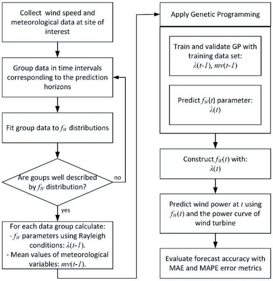
Figure 1.
The overarching methodology.
2.1. Wind Speed Probability Distribution and Wind Power
It is well known that wind speed is not easy to predict due to its not steady behavior. Therefore, a widely used approach to characterize the wind resource is its wind speed probability distribution functions (PDF). For many sites, the Weibull PDF provides a good fit to the annual frequency wind speeds of many sites. The Weibull PDF is given by [35]
where and are the shape and scale parameters of the distribution, respectively [36], and is the wind speed. As the name indicates, the shape parameter dictates the shape of the distribution. On the other hand, the scale parameter is in charge of the distribution width. Figure 2 shows the Weibull PDF for different values of the parameters. The blue lines correspond to the special case , known as Raleigh distributions, and different scale parameters (dotted line), (solid line) and (dash-dotted line). Different values for the shape factor , known as exponential distributions, and are shown in the red and yellow solid lines, respectively, for the same scale factor . Even though many sites can be well characterized by this distribution, there are some others with different behavior that can be characterized by bimodal probability distributions [37] or different distributions.
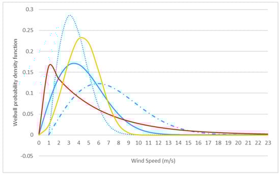
Figure 2.
Weibull probability distribution function for different values of the shape and scale parameters. The blue lines correspond to and for the dotted, solid and dash-dotted lines, respectively. The red and yellow solid lines correspond to , respectively, and .
Because of the wind variability, the power output of a wind turbine is highly variable and reliant on the weather conditions. In this regard, the power curve of a wind turbine describes how its power output varies with steady wind speed. This curve specifies: (a) the cut-in speed, at which the turbine first starts to rotate and generate power; (b) the cut-out speed, at which the turbine stops working for security reasons; and (c) the rated power output. Figure 3 shows the power curve of a small-scale wind turbine that is used in the case study later in this work. The power curve of a large-scale wind turbine exhibits the same characteristics but the produced power after the rated speed remains constant at the nominal value until the cut-off speed. For a Weibull distribution, it can be shown that the portion of time that power is produced in the interval and corresponds to the percentage of time that the wind speed lays in the range of velocities and , and it is given by [38,39]
where is the mean wind speed of the Weibull probability distribution and is given in terms of the scale and shape Weibull parameters by
and the Gamma function is defined as
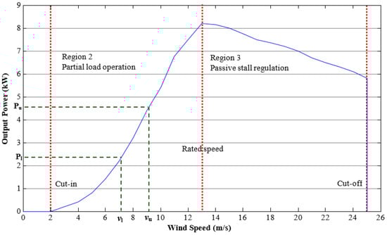
Figure 3.
Power curve of a small-scale small wind turbine.
2.2. Data Grouping, Prediction Horizons and Associated Parameters
There are several methods to estimate the Weibull parameters. Currently, research is going on to find the most reliable method to determine the Weibull shape parameter and the scale parameter [40,41,42] there are several methods, among the main ones are the graphical method (GM), the method of moments (MOM), the standard deviation method (STDM), the maximum likelihood method (MLM) and the equivalent energy method (EEM) [43].
An important point is the time interval of the data grouping. Weibull distributions are usually done for yearly or monthly data. However, seasonality is a characteristic of a time series in which the data experiences regular changes every year. In this work, it is important to find the shortest suitable time interval to describe the wind speed probability distribution by a Weibull distribution. This time interval depends on the wind resource behavior at the site. If, for instance, the location exhibits a wind resource with small variations in the wind speed, it is possible to group the data in smaller time intervals, such that the wind speed probability distributions at these time intervals can be accurately fitted by a Weibull distribution. On the other hand, if the location exhibits a wind resource with high variations in the wind speed, it is then necessary to group the data into a larger interval of time to accurately fit its wind speed distribution to a Weibull one.
As mentioned, the aim is to obtain good fits for the wind speed group data. First, we consider that the wind speed probability distribution is well characterized by a Rayleigh distribution. The Rayleigh probability distribution is a special case of the Weibull probability distribution in which the shape parameter is set to 2; therefore, we assume that the wind resource is well described by a Rayleigh distribution, implying . Next, to obtain the scale parameter , we use the GM to propose an initial value and then we optimize it using the EEM. The optimization process consists of setting the average wind power calculated from the Weibull distribution data, in the chosen time interval, as the objective function. Then, we optimize the value of by demanding that the objective function equals the average wind power per m2 calculated from the real data in the chosen time interval. Additionally, we compute the mean wind speed of the Weibull probability distribution . The mean wind speed of the fitted Weibull distribution is compared to the average wind speed calculated from the wind speed time series , as an indicator of whether the fit is good.
There are several methods for the goodness of fit for the Weibull distribution reported in the literature [44]. Probability plots provide a visual assessment of the model fit. The correlation coefficient measures how well the linear regression model fits the data. The maximum likelihood estimation method evaluates the parameters of the distribution model and assesses the fit of the distribution to the dataset. The Kolmogorov–Smirnov test is a non-parametric test of the equality of continuous distributions, which is used to compare a sample with a reference distribution. The Chi-Squared test is a statistical hypothesis test that uses a chi-squared distribution as a sampling distribution when the null hypothesis is true.
Once the fit is obtained for each group of n days, the mean solar radiation, ambient temperature, relative humidity and atmospheric pressure are calculated to climatologically characterize this period. In the next section, the forecast of the Weibull scale parameter is done by using GP.
2.3. Genetic Programming to Predict Weibull Distributions
The artificial evolution process is the foundation of GP, a machine learning and evolution-based search technique, which is a subclass of genetic algorithms [26]. In particular, individuals in a GP population are computer programs (or functions) not fixed in length or size. All solutions are considered but the search space is limited by defining the maximum depth height of the parse tree of the program and the maximum solution. When genetic operators are applied to the population of computer programs, the offspring structure, including size, shape and contents, may be different from their parents. Each hierarchical genotype is formed by functions that can be composed recursively of a set of functions , and a set of terminals . The function set can be any arithmetic, Boolean, mathematical, or more complex functions or routines. The terminal set consists of variables, constant values or functions, without input arguments.
Thus, GP can be applied to determine the structure, and the parameters, of nonlinear autoregressive models. In this particular case, we consider that the value of the scale parameter at a future time is given as a function of the parameters characterizing the period as follows
where refers to solar radiation, is the ambient temperature, is the atmospheric pressure, is the relative humidity, is the produced wind power, is the average wind speed from the data and is the mean speed from the Weibull distribution. Thus, the Weibull scale parameter is estimated at time by evaluating the function with their respective parameters at time . In this work, the function set contains only arithmetic operations , and the terminal set is composed of the independent variables I, T, P, PW, , and , all at the time . In addition, the generation of random numbers function is included in the terminal set to consider numerical values. Figure 4 shows an example of genotype and encoding used to forecast the Weibull scale parameter. In that specific case, the scale parameter is a function of the solar radiation, the ambient temperature and the atmospheric pressure.
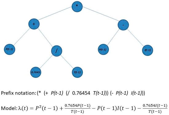
Figure 4.
Example of genotype and its encoding, prefix notation and mathematical model used in the GP.
Each individual is randomly created as a tree where internal nodes are functions and terminal nodes are arguments of the functions. The fitness function is generally defined as an error metric between the output produced by each individual and a reference corresponding, in this case, to the measure values. Thus, the fitness function can be any of the functions described in Section 2.5.
A new population is generated by selecting the fitter individuals through a selection method, which can be a proportional selection method such as roulette wheel, stochastic universal or tournament selection [45]. In this work, tournament selection is applied and consists of randomly selecting a competitor for each individual and performing a tournament. The best individual is the winner of the tournament and is considered for crossover and mutation.
Crossover is considered the main genetic operator exploiting the fittest individuals by exchanging randomly selected subtrees in both parents. Since the crossing point is different in the two parents, and individuals are different in structure and contents, the offspring will be different from their parents in structure but they will inherit characteristics from them [25]. A pair of structures is first selected from the current population. Next, in each parent, a node rooted is randomly chosen. Then, these nodes turn into the roots for the next sub-structures. Then, new structures of different sizes are created by the exchange of the previous sub-structures. This process is illustrated in Figure 5.
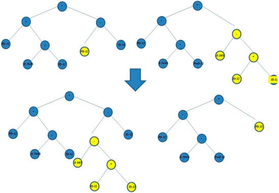
Figure 5.
Crossover process in the GP to forecast the scale parameter.
A secondary genetic operator corresponds to mutation. This operator explores the search space by introducing new information into the population. It randomly chooses a node, either a terminal or internal point, and substitutes its associated sub-structure with a randomly generated subtree up to a maximum size. This process is shown in Figure 6.
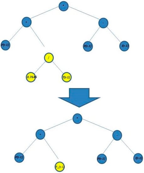
Figure 6.
Mutation process in the GP to forecast the scale parameter.
The steps for the GP algorithm to generate mathematical models of Weibull distributions are summarized in Table 1 and the parameters to solve the case study used in this work are specified in the next section.

Table 1.
Algorithm for GP to forecast of the scale parameter.
2.4. Estimating Wind Power at Long-Term
Given the PDF of the wind resource, the produced average power in the interval of time can be computed with the equation [46,47]
where corresponds to the power curve of the wind turbine and is the probability distribution function of the wind speed, which in this case corresponds to the Weibull distribution.
In this work, given the low-speed wind data, we consider a small-scale wind turbine whose power curve is shown in Figure 3. However, it is worth mentioning that the same methodology applies to a large-scale wind power curve. We concentrate on the wind speed interval . In this speed interval, the power curve can be approximated by the following equation:
where the coefficient of determination of the fit is high, , indicating that goodness of the fit.
2.5. Forecasting Error
In the following, different metrics are used to evaluate the forecasting accuracy [48]. First, we compute the forecast or residual error () defined as the difference between the measured and the forecast value for the corresponding period
where is the forecast error of the variable at period , is the measured value of the variable at period and is the forecast variable at period . Since the forecast error is on the same scale as the data, the accuracy measures depend on the scale of the variable. To make a comparison between series on different scales we also compute the Mean Absolute Error (MAE) given by
Finally, we also calculate the percentage error Mean Absolute Percentage Error (MAPE), which is also scale-independent, given by
to compare forecast performance between different datasets.
3. Experiments and Results
The long-term power estimation methodology presented in the previous sections is general enough to be applied to any site, with any arbitrary wind distribution and with wind turbines of any size that can be driven with the available wind resource. In this regard, the wind resource at many locations in Mexico has already been studied for the deployment of medium and large wind turbines [49]. In addition, Sanchez et al. [50] proposed a statistical analysis based on wind velocity vectors to model the wind resource with Markov chains, and tested their model in Baja California and Oaxaca. A wind speed analysis in La Ventosa is done in [37,51]. The wind power potential of Baja California is studied in [52] and the analysis and forecasting of the wind velocity in Chetumal is performed in [53].
Nowadays, it is becoming of major relevance the deployment of small-scale wind turbines to provide cleaner and cheaper energy for on-grid and off-grid applications such as businesses, small industries and factories, farms and ranches, urban and suburban living communities, rural residential electrification, communication stations, water treatment, and pumping, etc. [54]. To decide whether to deploy small-scale wind turbines, a technical assessment must be carried out as a first phase [55]. The potential to supply part, most or all required energy with the available wind resource at a given site must be clearly stated, considering that the energy produced by a small-scale wind turbine can be estimated from the turbine power curve and the wind speed distribution at the site [56]. In [57], we introduced a Bayesian decision system based on probabilistic reasoning to assess the suitability of small-scale wind turbines taking into consideration the availability of wind resources at various sites and the energy pricing structure in Mexico.
In this section, we study the wind resource at a specific location in Mexico to demonstrate the feasibility of the proposed approach long-term estimation methodology. In particular, we consider data from the meteorological station located in Enrique Estrada in the state of Zacatecas, Mexico, with a geographical location at latitude N: 22° 59´36´´ and longitude W: 102° 53´02´´, and at an altitude of 2319 m above sea level. The terrain is complex, with mountains to the west and flatlands to the north, east and south. The tower is 30 m high and the recorded measurements are wind speed, ambient temperature, solar radiation, relative humidity and atmospheric pressure, among others. The data are monitored every 2 s to calculate and record mean values every 10 min.
We consider data from 2010 and 2011. Figure 7a,b shows the wind speed distribution for all the dataset corresponding to the site under study at 30 m height. The wind speed PDFs follow Weibull distributions and therefore the proposed methodology can be applied.
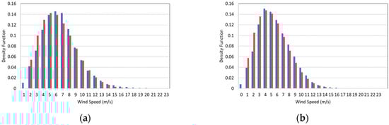
Figure 7.
Normalized histogram of wind speeds, in blue, and fitted Weibull distribution, in red, for: (a) 2010; and (b) 2011. The Weibull parameters are and and and , for 2010 and 2011, respectively.
The first thing to note is that the Rayleigh assumption, , provides a good fit to the data using GM, as shown in Figure 7a,b. As mentioned in Section 2.2, we calculate the optimal value of by using the EEM, i.e. requiring that the objective function, defined as the mean wind power from the distribution, is equal to the average wind power from data, shown in the fourth column in Table 2. Additionally, Table 2 shows the average wind speed calculated from the wind speed time series , and the mean wind speed of the Weibull probability distribution . Note that the average and mean wind speeds per year are very close. This indicates that the fit to the wind speed distribution is good.
Table 2.
Characteristics of the wind resource per year: average power , average wind speed from data and mean wind speed from Weibull distribution .
3.1. Data Grouping, Prediction Horizons and Associated Parameters
3.1.1. Seasonality
For forecasting, it is important to analyze the time series to identify if there are datasets that experiences regular changes every year. In particular, the wind varies according to the season of the year. To study whether the wind resource at the site follows a seasonality behavior, we fit a Weibull distribution at each period corresponding to each season and calculate by assuming the Rayleigh criteria . We consider that each season lasts three months and the dates are defined by the equinoxes and solstices. Table 3 shows the scale parameter, the average wind power, the average wind speed and the mean wind speed. As expected, the wind speed is smaller in the summer–fall period than during winter–spring, and similarly for the wind power. In addition, the scale parameter is smaller during summer–fall than during winter–spring. Therefore, for this study, henceforth we consider the wind resource in two different periods: summer–fall (SF) and winter–spring (WS).
Table 3.
Characteristics of the wind resource per season: scale parameter , average power , average wind speed from data and mean wind speed from Weibull distribution .
3.1.2. Grouping and Prediction Horizons
The horizon of the prediction is given by the time interval of the data group. Given that we only count on a two-year dataset, we consider groups of data up to 30 days to have enough data for evolutionary programming. However, as we are dealing with distributions, the advantage of this approach is that the bigger the dataset is, the longer the prediction horizons can be. Thus, one can deal with larger time intervals if there were years of data.
30 Days Ahead
Considering the data from 2010 and 2011, we have 12 groups of 30 days in each of the periods WS and SF. We fit Weibull distributions to the wind speed histograms obtained with wind speed data every 30 days according to the methodology described above. Figure 8 shows six groups of samples of normalized histograms of the wind speeds, in blue, and fitted Weibull distribution functions, in orange, for group periods of 30 days each during the WS season.
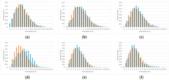
Figure 8.
Six groups of samples of normalized histograms of wind speed, in blue, and fitted Weibull distribution, in orange, for group periods of 30 days each during WS season. Each graph corresponds to the following period (a) 01/01/2010–01/30/2010; (b) 01/31/2010–03/01/2010; (c) 03/02/2010–03/31/2010; (d) 04/01/2010–04/30/2010; (e) 05/01/2010–05/30/2010; (f) 12/21/2010–01/19/2011.
25 Days Ahead
Considering the data from 2010 and 2011, we have 12 groups of 25 days in each of the periods WS and SF. Figure 9 shows six groups of samples of normalized histograms of the wind speeds, in blue, and fitted Weibull distribution functions, in orange, in periods of 25 days each during the WS season for 2010.
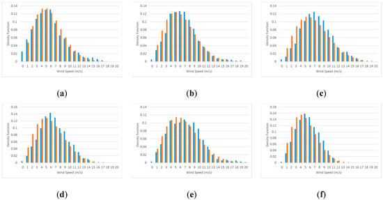
Figure 9.
Six groups of samples of normalized histograms of wind speeds, in blue, and fitted Weibull distribution, in orange, for group periods of 25 days each during WS season. Each graph corresponds to the following period (a) 01/01/2010–01/25/2010; (b) 01/26/2010–02/19/2010; (c) 02/20/2010–03/16/2010; (d) 03/17/2010–04/10/2010; (e) 04/11/2010–05/05/2010; (f) 05/06/2010 – 05/30/2010.
20 Days Ahead
Considering the data from 2010 and 2011, we have 16 groups of 20 days in each of the periods WS and SF. Figure 10 shows six groups of samples of normalized histograms of the wind speeds, in blue, and fitted Weibull distribution functions, in orange, in periods of 20 days each during the WS season for 2010.
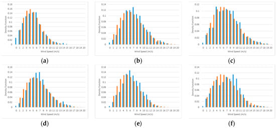
Figure 10.
Six groups of samples of normalized histograms of wind speeds, in blue, and fitted Weibull distribution, in orange, for group periods of 20 days each during WS season. Each graph corresponds to the following period (a) 01/01/2010–01/20/2010; (b) 01/21/2010–02/09/2010; (c) 02/10/2010–03/01/2010; (d) 03/02/2010–03/21/2010; (e) 03/22/2010–04/10/2010; (f) 04/11/2010–04/30/2010.
15 Days Ahead
Considering the data from 2010 and 2011, we have 24 groups of 15 days in each of the periods WS and SF. Figure 11 shows six groups of samples of normalized histograms of the wind speeds, in blue, and fitted Weibull distribution functions, in orange, for group periods of 15 days each during the WS season for 2010.
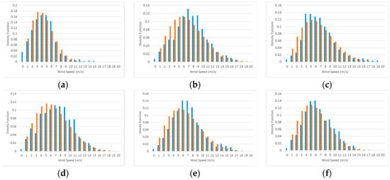
Figure 11.
Six groups of samples of normalized histograms of wind speeds, in blue, and fitted Weibull distribution, in orange, for group periods of 15 days each during WS season. Each graph corresponds to the following period (a) 01/01/2010–01/15/2010; (b) 01/16/2010–01/30/2010; (c) 01/31/2010–02/14/2010; (d) 02/15/2010–03/01/2010; (e) 03/02/2010–03/16/2010; (f) 03/17/2010–03/31/2010.
10 Days Ahead
Considering the data from 2010 and 2011, we have 36 groups of 10 days in each of the periods WS and SF. Figure 12 shows six groups of samples of normalized histograms of the wind speeds, in blue, and fitted Weibull distribution functions, in orange, for group periods of 10 days each during the WS season for 2010.
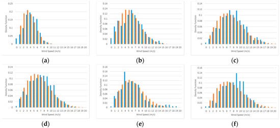
Figure 12.
Six groups of samples of normalized histograms of wind speeds, in blue, and fitted Weibull distribution, in orange, for group periods of 10 days each during WS season. Each graph corresponds to the following period (a) 01/01/2010–01/10/2010; (b) 01/11/2010–01/20/2010; (c) 01/21/2010–01/30/2010; (d) 01/31/2010–02/09/2010; (e) 02/10/2010–02/19/2010; (f) 02/20/2010–03/01/2010.
3.1.3. Parameters
Each group of days is characterized by representative parameters of the weather conditions in that period. First, the scale and shape parameter Weibull parameters, as well as the average and mean wind speeds, categorize the wind resource. On the other hand, solar radiation, ambient temperature, relative humidity and atmospheric pressure are treated as normal distributions and, thus, their mean values are computed and considered. Table 4 shows the characteristic parameters for a sample of group periods of 10 days each during the WS season. The whole set of data is included in Supplementary Materials. The average of the wind power and wind speed, as well as the mean wind speed calculated from the distribution, are shown as well.
Table 4.
Characteristic parameters for group periods of 10 days each during the WS season.
This dataset contains the information to characterize the conditions for each n-day group at a given season.
3.2. Predicting Weibull Distributions
The GP code was developed in MATLAB, following the algorithm described in Table 1. Table 5 shows the specifications of the GP process to forecast the scale parameter of wind speed Weibull distributions.
Table 5.
Specifications of the GP process to forecast the scale parameter of wind speed Weibull distributions.
Using GP, the scale parameter parameters of the Weibull distributions are predicted at different time horizons: 30, 25, 20, 15 and 10 days ahead. Figure 13 shows the predicted scale parameters at different horizons. The blue and the gray dashed lines correspond to the values of the measured and predicted values of the scale parameter in the WS season. The yellow and gray dashed lines correspond to the values of the measured and predicted values of the scale parameter in the SF season. The horizons of the predictions are as follows: (a) 30 days ahead; (b) 25 days ahead; (c) 20 days ahead; (d) 15 days ahead; and (e) 10 days ahead.
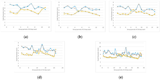
Figure 13.
Predicted scale parameters at different horizons. The blue and the gray dashed lines correspond to the values of the measured and predicted values of the scale parameter in the WS season. The yellow and the gray dashed lines correspond to the values of the measured and predicted values of the scale parameter in the SF season. The horizons of the prediction are as follows: (a) 30 days ahead; (b) 25 days ahead; (c) 20 days ahead; (d) 15 days ahead; and (e) 10 days ahead.
Note that the scale parameter is larger in the WS season than in the SF season, meaning that the wind speed is higher in the WS season. Additionally, the predicted values are very close to the measured values. In particular, in Figure 13, we see that the prediction is more accurate for larger prediction horizons than for a short one. With the forecasted scale parameter, the forecasted wind speed distribution is completely defined and the estimation of the wind power at different periods is calculated in the next section.
3.3. Estimating Wind Power
The forecasted wind speed Weibull distribution is completely defined with the forecasted scale parameter and the Rayleigh shape parameter . This dataset contains the information that characterizes the wind speed conditions on an n-day group at a given season. In addition, considering that the wind speed at the site of interest has annual averages close to , there is enough power to drive a small-scale wind turbine generator, as stated in [11], with a power curve such as the one shown in Figure 3. Thus, the predicted wind power at different intervals of time is computed using Equations (6) and (7). Figure 14 shows the estimated and measured wind power for horizons of: (a) 20 days ahead; (b) 25 days ahead; (c) 20 days ahead; (d) 15 days ahead; and (e) 10 days ahead. The blue and yellow lines correspond to the measured wind power in the WS and SF seasons, respectively, and the grey dashed lines correspond to the estimated wind power. Note that, as expected from the predicted and measured scale parameters, the produced wind power in the WS season is higher than the produced in the SF season. Nevertheless, although there is less power production during the SF season, the behavior is steadier in that season. The first thing to note is that the estimated wind power is smaller than the measured one. Moreover, the estimated wind power in the SF season is closer to the measured value than in the WS season.
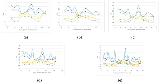
Figure 14.
Estimated and measured wind power for horizons of: (a) 30 days ahead; (b) 25 days ahead; (c) 20 days ahead; (d) 15 days ahead; and (e) 10 days ahead. The blue and yellow lines correspond to the measured wind power in the WS and SF seasons, respectively, and the grey dashed lines correspond to the estimated wind power.
To quantify the forecasting accuracy, we compute the forecasting errors in the next section.
3.4. Forecasting Errors
Figure 15 shows the forecast error , as defined in Equation (8), for the estimated wind power for horizons of: (a) 30 days ahead; (b) 25 days ahead; (c) 20 days ahead; (d) 15 days ahead; and (e) 10 days ahead. The blue and yellow lines correspond to the WS and SF seasons, respectively. In Figure 15a–e, as the interval of time decreases, the forecasting error increases. This means that the estimation of wind power is more accurate at larger intervals of time, i.e. 30 days ahead, than at smaller intervals of time, i.e. 10 days ahead. Additionally, the forecasting error is larger in the WS season than in the SF season. This is because wind power behavior is steadier in the SF season than in the WS season resulting in better forecasting accuracy during the SF season.
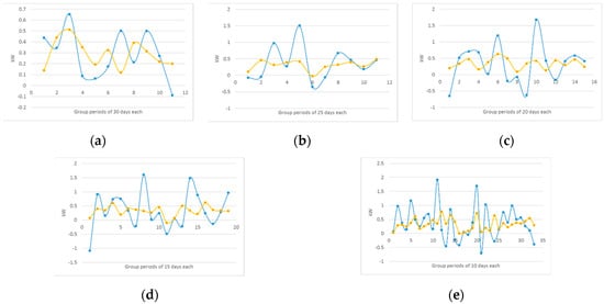
Figure 15.
Forecast error for the estimated wind power for horizons of: (a) 30 days ahead; (b) 25 days ahead; (c) 20 days ahead; (d) 15 days ahead; and (e) 10 days ahead. The blue and yellow lines correspond to the WS and SF seasons, respectively.
Table 6 shows the MAE and MAPE errors for the estimated wind power at future times, using Equations (9) and (10), for the WS and SF seasons. As expected from the discussion concerning Figure 14 and Figure 15, the errors are smaller in the SF season than in the WS season, confirming that the prediction is better in the SF season. Additionally, as mentioned above, the proposed approach to estimate the produced wind power provides a better accuracy as the interval of time is larger. Thus, a 30-day-ahead estimation results better than a 10-day-ahead estimation, confirming that the presented methodology is a promising candidate for long-term estimation of wind power.
Table 6.
MAE and MAPE values for the estimated values of wind power at different future times.
4. Discussion
In general, long-term forecasting is a difficult task since, for most of the methodologies, the forecasting error becomes larger as the prediction horizon increases. However, as shown by the results in this work, the proposed forecasting methodology provides better results as the prediction horizon becomes larger. This trend relays on the fact that, even though the prediction of the scale parameter could be better for smaller horizons, the fitting of the wind speed distribution to a Weibull distribution is better as more data is provided, or equivalently as a larger interval of time is considered. Hence, the proposed approach is a promising methodology for long-term wind power forecasting.
Likewise, it is important to recall that the randomness and intermittency of the wind resource is the major challenge for the integration of wind power into electric power systems [58]. As such, wind farms with large-scale wind turbines are typically connected to the high-voltage transmission networks, while farms with small-scale wind turbines are ordinarily connected to the distribution network, mainly as distributed energy sources [59]. In both cases, accurate prediction of wind power generation for horizons up to 30 days ahead is a crucial ingredient for effective dispatch planning, system planning, financial investments, operation management, optimal operation, maintenance cost reduction and feasibility analysis of the wind farm [2,3]. Up to these days, most of the studies on long-term wind power forecasts have been carried out for large-scale wind turbines that provide the largest contribution of bulk renewable energy. It is only a matter of time that long-term wind power prediction for small-scale wind turbines will become a must, as programs to achieve 100% energy supply from renewables become commonplace all around the globe to mitigate climate change and eliminate dependency on oil and its derivatives [60]. Therefore, the case study presented in this work, with the chosen small-scale wind turbine, provides insights in this direction.
Similarly, it is interesting to compare the obtained results of our novel approach of probabilistic forecasting for long-term wind power with results from different studies, even if most of the published work has been done using deterministic forecasting. In [61], different models for wind power forecasting, and a case study, are introduced. In particular, the authors performed long-term forecasting using the wind speed and other meteorological variables with four methods involving ARIMA, neural networks and hybrid combinations of them. They calculated the forecasting errors, finding promising results for 10 and 20 days ahead forecasting by using three of their methods. However, it is important to highlight that a small MAPE in their predicted wind speed does not imply a small MAPE in the predicted wind power since the wind power is proportional to the wind speed cubed. In [62], an adaptive wavelet neural network is used for long term wind power forecasting. Their predictions achieve good accuracy as shown in the calculated MAPE but they forecast up to 72 h. In [63], a locally recurrent neural network is used to predict wind speed and power up to a few days showing good results as shown from their reported small values of MAE.
The following main advantages of our probabilistic approach are recalled: (a) the information about the wind resource is not lost, in contrast with the deterministic approaches that use average values of wind speed [64]; (b) the prediction horizon is flexible as far as the dataset and the nature of the wind resource nature allow it; (c) the introduced methodology can be used for small and large scale wind turbine generators; (d) the proposed methodology does not require a large amount of data since GP is a search technique from machine learning that evolves a function to minimize the fitness function, which in this case corresponds to the prediction errors, in contrast with other techniques from artificial intelligence, such as neural networks, that requires a training and validation process [65]; and (e) there are few published works in long-term wind power forecasting (most of them are up to a few days) and small-scale wind power, therefore this work boosts research in these directions.
There are many ways to extend this work to overcome its limitations. First, one can relax the Rayleigh criteria and predict the scale and shape parameter of the distributions, since there are sites where fits better the characterization of the wind resource [66]. Moreover, even though there are several sites with wind resources well-characterized by Weibull distributions [67,68,69,70,71,72,73,74,75,76], there are sites with wind resources not well-described by Weibull distributions. For instance, in La Ventosa, Mexico, the wind speed distribution follows a bimodal Weibull distribution [51]. In addition, on some Greek islands located in the Eastern Mediterranean, the wind resource is better characterized by two components, each of them with two-parameter Weibull PDF known as class 2 [77]. Similarly, Carta et al. presented a review of wind speed probability distributions on the Canary Islands [34], finding that the Weibull distribution is not suitable for all wind regimes. Moreover, a review of recent progress in wind speed distribution selection finds that Weibull distribution is the most frequently adequate distribution but there are others such as Wakeby and Kappa that better fit some sites [78]. Finally, Drobinski et al. remarked that the Weibull distribution does not describe well the high wind potential and proposed Rayleigh–Rice super-statistical distributions for locations where the wind is not isotropic [79]. Thus, this work could be extended to the more general Kernel probability distribution to be applied in a bigger set of sites. In addition, it would be interesting to consider a larger database to provide longer-term forecasting. However, one has to be careful about that since seasonality plays an important role in data grouping and prediction horizons. Finally, even though the achieved results are very promising with feasible forecasting error after comparing with measured data, it would be interesting to perform similar probabilistic forecasting with other techniques, such as neural networks, or multi regression, to compare the performance of them.
5. Conclusions
In this paper, we introduce a novel probabilistic forecasting method for long-term wind power estimation using wind speed statistics, genetic programming, and wind turbine properties. The methodology mainly consists of curve fitting the wind speed data, forecasting the wind speed probability distribution function at a future time, and estimating the produced wind power. A case study of a site in Mexico with an annual wind speed of 5.1 m/s and a wind resource well-described by a Weibull probability distribution, as well as small-scale wind turbine technology, are employed to show the feasibility of the proposed methodology obtaining very good results as can be seen in the estimation accuracy graded with MAE and MAPE metrics.
The wind speed variability and intermittency are captured by Weibull distributions. Time intervals of 30, 25, 20, 15 and 10 days of 10-min average data are used to fit the Weibull distributions. These intervals correspond to the forecasted horizons of the same days ahead length. However, a different interval of any number of days can be used as long as the available data and the seasonality of the wind resource allow a good fitting to the probabilistic density functions. However, in an interval (prediction horizon) smaller than 10 days, it is difficult to treat wind speed data statistically. The larger is the time horizon, the better is the statistical treatment of the data, and the better is the forecasted result. However, the length of the interval is limited by the seasonality of the wind resource at the site of interest. For the presented case study, the best forecast is obtained with time intervals, and prediction horizons, of 30 days ahead. It is important to note that the same procedure can be applied to the case where the wind resource is not appropriately described by Weibull probability distributions by using better-suited distributions and predicting their characteristic parameters.
The prediction of the wind speed probability distribution function is carried out using genetic programming, which is a heuristic technique that evolves the mathematical expression of the probability distribution using genetic operators to find the expression that minimizes the distribution fitness function in the prediction horizon. In this paper, the genetic programming forecasts the scale parameter λ of the wind speed Weibull distribution. For the presented case study, the fittest probability distribution functions are those for 30 days intervals, and for the summer–fall seasonality, given the nature of the wind resource at the site.
Finally, the estimated produced wind power at a future time is calculated by integrating the power curve of the wind turbine with the predicted probability distribution function.
Supplementary Materials
The meteorological database is available online at http://doi.org/10.5281/zenodo.3691886. The data will be published once the paper has been accepted for publication.
Author Contributions
Conceptualization, M.B. and O.A.J.; methodology, M.B., K.R.-V., R.G.-R., and O.A.J.; software, M.B., K.R.-V., R.G.-R., J.d.l.C.-S., and J.A.-E.; validation, M.B. and R.G.-R.; formal analysis, M.B., K.R.-V., R.G.-R., and O.A.J.; investigation, M.B., R.G.-R., and J.C.S.; resources, O.A.J.; data curation, M.B., R.G.-R., J.C.S., and J.A.-E.; writing—original draft preparation, M.B.; writing—review and editing, M.B., K.R.-V., R.G.-R., J.C.S., and J.A.-E.; visualization, M.B., and O.A.J.; supervision, M.B.; and project administration, M.B. All authors have read and agreed to the published version of the manuscript.
Funding
This research received no external funding.
Acknowledgments
We acknowledge Daniel Reyes Guillén for his support in the presentation of results.
Conflicts of Interest
The authors declare no conflict of interest.
Nomenclature
| Wind speed | ||
| − | Weibull probability density function | |
| − | Probability density function | |
| Scale parameter of the Weibull probability density function | ||
| − | Shape parameter of the Weibull probability density function | |
| − | Percentage of time (of the total time used to construct the Weibull PDF) where an amount of wind power is produced. | |
| Lower wind speed in a time interval | ||
| Upper wind speed in a time interval | ||
| Mean wind speed from distribution | ||
| Average mean wind speed from data | ||
| − | Gamma function | |
| Solar radiation | ||
| Ambient temperature | ||
| Atmospheric pressure | ||
| Relative humidity | ||
| Produced power from wind turbine | ||
| Produced power from a wind turbine in an interval of time | ||
| Power curve of the wind turbine as a function of the wind speed | ||
| − | Set of functions used by the GP algorithm | |
| − | n function used by the GP algorithm | |
| − | Set of terminals used by the GP algorithm | |
| − | n terminal used by the GP algorithm | |
| − | Fitness function used by the GP algorithm | |
| − | Generation of GP | |
| − | Population at generation | |
| − | Individual of the population | |
| − | Coefficient of determination | |
| Units of forecasted variable | Forecast or residual error of a variable at a period | |
| Units of forecasted variable | Measured value of wind speed at a time period | |
| Units of forecasted variable | Forecasted value of wind speed at a time period | |
| − | Sample number of measured and forecasted values of variable | |
| Units of forecasted variable | Mean Absolute Error | |
| % | Mean Absolute Percentage Error |
References
- Guo, P.; Huang, X.; Wang, X. A review of wind power forecasting models. Energy Procedia 2011, 12, 770–778. [Google Scholar]
- Song, Y.; Liu, F.; Hou, R.; Wang, J. Analysis and application of forecasting models in wind power integration: A review of multi-step-ahead wind speed forecasting models. Renew. Sustain. Energy Rev. 2016, 60, 960–981. [Google Scholar]
- Grundmeyer, M.; Gervert, M.; Lerner, J. The importance of wind forecasting. Renew. Energy Focus 2009, 10, 64–66. [Google Scholar]
- Ramirez, P.; Carta, J.A. The use of wind probability distributions derived from the maximum entropy principle in the analysis of wind energy. a case study. Energy Convers. Manag. 2005, 47, 2564–2577. [Google Scholar] [CrossRef]
- Weibull, W. A statistical distribution function of wide applicability. J. Appl. Mech. Trans. ASME 1951, 18, 293–297. [Google Scholar]
- Sigl, A.B.; Corortis, R.B.; Klein, J. Probability models for wind velocity magnitude and persistence. Sol. Energy 1978, 20, 483–493. [Google Scholar]
- Hennessey, J.P., Jr. A comparison of the Weibull and Rayleigh distributions for estimating wind power potential. Wind Eng. 1978, 2, 156–164. [Google Scholar]
- Yalcin, A.; Justus, C.G.; Hargreaves, W.R. Nationwide assessment of potential output from wind-powered generators. J. Appl. Meteorol. 1976, 15, 673–678. [Google Scholar]
- Bhattacharya, P. A study on Weibull distribution for estimating the parameters. J. Appl. Quant. Methods 2010, 5, 234–241. [Google Scholar] [CrossRef]
- Rainer, M.; Giebel, S.M.; Aydin, N.S. Simulation and prediction of wind speeds: A neural network for Weibull. JIRSS 2013, 12, 293–319. [Google Scholar]
- Alam, M.M.; Ameer Uddin, S.M.; Mondal, S.K.; Azad, A.K.; Rasul, M.G. Analysis of wind energy conversion system using Weibull distribution. Proceedia Eng. 2014, 90, 725–732. [Google Scholar]
- Arik, I.; Yenilmez, I.; Mert Kantar, Y.; Usta, I. Analysis of the modified Weibull distribution for estimation of wind speed distribution. Proc. Int. Conf. Eng. MIS 2015, 49. [Google Scholar] [CrossRef]
- Islam, R.; Azad, A.K.; Rasul, M.G.; Shishir, I.R. Analysis of wind energy prospect for power generation by three Weibull distribution methods. Energy Proceedia 2015, 75, 722–727. [Google Scholar]
- Vermorel, J. Probabilistic Forecasting. 2015. Available online: www.lokad.com/probabilistic-forecasting-definition (accessed on 23 February 2020).
- Little, M.A.; McSharry, P.E.; Taylor, J.W. Generalized linear models for site-specific density forecasting of UK daily rainfall. Mon. Weather Rev. 2009, 37, 1029–1045. [Google Scholar] [CrossRef]
- Strumbelj, E. On determining probability forecasts from betting odds. Int. J. Forecast. 2014, 30, 934–943. [Google Scholar] [CrossRef]
- Garrat, A.; Lee, K.; Pesaran, M.P.; Shin, Y. Forecast Uncertainties in Macroeconometric Modelling: An Application to the UK Economy. 2000. Available online: www.le.ac.uk/economics/research/RePEc/lec/leecon/econ00-4.pdf (accessed on 23 February 2020).
- Alders, M.; Keilman, N.; Cruijsen, H. Assumptions for long-term stochastic population forecasts in 18 European countries. Eur. J. Popul. 2007, 23, 33–69. [Google Scholar] [CrossRef]
- Hong, T.; Pinson, P.; Fan, S.; Zareipour, H.; Troccoli, A.; Hyndman, R.J. Probabilistic energy forecasting: Global Energy Forecasting Competition 2014 and beyond. Int. J. Forecast. 2016, 32, 896–913. [Google Scholar] [CrossRef]
- Zhou, Z. Application of probabilistic wind power forecasting in electricity markets. Wind Energy 2013, 16, 321–338. [Google Scholar] [CrossRef]
- Wan, C.; Lin, J.; Wang, J.; Song, Y.; Dong, Z.Y. Direct Quantile Regression for Nonparametric Probabilistic Forecasting of Wind Power Generation. IEEE Trans. Power Syst. 2016, 32, 2767–2778. [Google Scholar] [CrossRef]
- Xydas, E.; Qadrdan, M.; Marmaras, C.; Cipcigan, L.; Jenkins, N.; Ameli, H. Probabilistic wind power forecasting and its application in the scheduling of gas-fired generators. Appl. Energy 2017, 192, 382–394. [Google Scholar] [CrossRef]
- Bäck, T. Evolutionary Algorithms in Theory and Practice; Oxford University Press: New York, USA, 1996. [Google Scholar]
- Koza, J.R. Hierarchical Genetic Algorithms Operating on Populations of Computer Programs. In Proceedings of the Eleventh International Joint Conference on Artificial Intelligence, Detroit, MI, USA, 20–25 August 1989; Morgan Kaufmann: MA, USA, 1989; Volume 1, pp. 768–774. [Google Scholar]
- Koza, J.R. Genetic Programming: On the Programming of Computers by Means of Natural Selection; MIT Press: Cambridge, MA, USA, 1992. [Google Scholar]
- Holland, J.H. Adaptation in Natural and Artificial Systems; The University of Michigan Press: Cambridge, MA, USA, 1975. [Google Scholar]
- Koza, J.R. Genetic Programming as a means for programming computers by natural selection. Stat. Comput. 1994, 4, 87–112. [Google Scholar] [CrossRef]
- Graff, M.; Escalante, H.J.; Ornelas-Tellez, F.; Tellez, E.S. Time series forecasting with genetic programming. Nat. Comput. 2017, 16, 165–174. [Google Scholar] [CrossRef]
- Danandeh, M.A.; Bagheri, F.; Resatoglu, R. A Genetic Programming Approach to Forecast Daily Electricity Demand. In 13th International Conference on Theory and Application of Fuzzy Systems and Soft Computing—ICAFS-2018. Advances in Intelligent Systems and Computing; Springer: Cham, Switzerland, 2018; p. 896. [Google Scholar]
- Karabulut, K.; Alkan, A.; Yilmaz, A.S. Long Term Energy Consumption Forecasting Using Genetic Programming. Math. Comput. Appl. 2008, 13, 71–80. [Google Scholar] [CrossRef]
- Lee, D.G.; Lee, B.W.; Chang, S.H. Genetic programming model for long-term forecasting of electric power demand. Electron Power Syst. Res. 1997, 40, 17–22. [Google Scholar] [CrossRef]
- Graff, M.; Peña, R.; Medina, A. Wind Speed Forecasting using Genetic Programming. IEEE Congr. Evol. Comput. 2013, 408–415. [Google Scholar] [CrossRef]
- Martínez-Arellano, G.; Nolle, L. Genetic Programming for Wind Power Forecasting and Ramp Detection. In Research and Development in Intelligent Systems XXX; Springer: Heidelberg, Germany, 2013. [Google Scholar]
- Carta, J.A.; Ramírez, P.; Velázquez, S. A review of wind speed probability distributions used in wind energy analysis case studies in the Canary Islands. Renew. Sustain. Energy Rev. 2009, 13, 933–955. [Google Scholar] [CrossRef]
- Rinne, H. The Weibull Distribution, A Handbook; CRC Press: Boca Raton, FL, USA, 2009. [Google Scholar]
- Unnikrishna, P.S.; Papoulis, A.P. Probability, Random Variables, and Stochastic Processes; McGraw-Hill: Boston, MA, USA, 2002. [Google Scholar]
- Jaramillo, O.A.; Borja, M.A. Bimodal versus Weibull wind speed distributions: An analysis of wind energy potential in la venta, Mexico. Wind Eng. 2004, 28, 225–234. [Google Scholar] [CrossRef]
- Mathew, S. Wind Energy: Fundamentals, Resource Analysis and Economics; Springer: Berlin/Heidelberg, Germany, 2006. [Google Scholar]
- Johnson, G.L. Wind Energy Systems; Kansas State University: Manhattan, KS, USA, 2006. [Google Scholar]
- Celik, A. Weibull representative compressed wind speed data for energy and performance calculations of wind energy systems. Energy Convers. Manag. 2003, 44, 3057–3072. [Google Scholar] [CrossRef]
- Ulgen, K.; Hepbasli, A. Determination of Weibull parameters for wind energy analysis of Izmir, Turkey. Int. J. Energy Res. 2002, 26, 495–506. [Google Scholar] [CrossRef]
- Langlois, R. Estimation of Weibull parameters. J. Mater. Sci. Lett. 1991, 10, 1049–1051. [Google Scholar] [CrossRef]
- Azad, A.K.; Rasul, M.G.; Yusaf, T. Statistical Diagnosis of the Best Weibull Methods for Wind Power Assessment for Agricultural Applications. Energies 2014, 7, 3056–3085. [Google Scholar] [CrossRef]
- Kececioglu, D. Reliability and Life Testing Handbook; Prentice Hill, Inc.: Upper Saddle River, NJ, USA, 1993; Volume I. [Google Scholar]
- Baker, J.E. Reducing Bias and Inefficiency in the Selection Algorithm. In Proceedings of the 2nd International Conference on Genetic Algorithms, NJ, USA, 1987; Grefenstette, Ed.; 1987; pp. 14–21. [Google Scholar]
- Rau, V.G.; Jangamshetti, S.H. Normalized power curves as a tool for identification of optimum wind turbine generator parameters. IEEE Trans. Energy Convers. 2001, 16, 283–288. [Google Scholar] [CrossRef]
- El-Sharkawi, M.A. Wind Energy, an Introduction; CRC Press: Boca Raton, FL, USA, 2015. [Google Scholar]
- Armstrong, J.S.; Collopy, F. Error measures for generalizing about forecasting methods: Empirical comparisons. Int. J. Forecast. 1992, 1, 69–80. [Google Scholar] [CrossRef]
- Hernandez-Escobedo, Q.; Manzano-Agugliaro, R.; Zapata-Sierra, A. The wind power of Mexico. Renew. Sustain. Energy Rev. 2010, 14, 2830–2840. [Google Scholar] [CrossRef]
- Robles, M.; Sanchez-Perez, P.A.; Jaramillo, O.A. Real time Markov chains: Wind states in anemometric data. Renew. Sustain. Energy 2016, 8, 024403. [Google Scholar]
- Borja, M.A.; Jaramillo, O.A. Wind speed analysis in La Ventosa, Mexico: A bimodal probability distribution case. Renew. Energy 2004, 29, 1613–1630. [Google Scholar]
- Saldana, R.; Jaramillo, O.A.; Miranda, U. Wind power potential of Baja California Sur, Mexico. Renew. Energy 2004, 29, 2087–2100. [Google Scholar]
- Jaramillo, O.A.; Cadenas, E.; Rivera, W. Analysis and forecasting of wind velocity in Chetumal, Quintana Roo, using the exponential smoothing method. Renew. Energy 2010, 35, 925–930. [Google Scholar]
- Tzen, E. Small wind turbines for on grid and off grid applications. IOP Conf. Ser. Earth Environ. Sci. 2020. [Google Scholar] [CrossRef]
- Olsen, T.L.; Preus, R. Small Wind Site Assessment Guidelines; NREL/TP-5000-63696: September 2015. Available online: https://www.nrel.gov/docs/fy15osti/63696.pdf (accessed on 23 February 2020).
- Ozgener, O. A small wind turbine system (SWTS) application and its performance analysis. Energy Conversion and Management. 2006, 47, 1326–1337. [Google Scholar] [CrossRef]
- Borunda, M.; De La Cruz, J.; Garduno-Ramirez, R.; Nicholson, A. Technical assessment of small-scale wind power for residential use in Mexico: A Bayesian intelligence approach. PLoS ONE 2020, 15, e0230122. [Google Scholar] [CrossRef]
- Jain, P.; Wijayatunga, P. Grid Integration of Wind Power: Best Practices for Emerging Wind Markets; Asian Development Bank: Mandaluyong, Philippines, 2016; Volume 43, pp. 2–36. [Google Scholar]
- Danish Energy Agency. Energy Policy Toolkit on System Integration of Wind Power; Experiences from Denmark; Danish Energy Agency: København, Denmark, 2015; ISBN 978-87-93071-93-3. [Google Scholar]
- Idriss, A.I.; Ahmed, R.A.; Omar, A.I.; Said, R.K.; Akinci, T.C. Wind energy potential and micro-turbine performance analysis in Djibouti-city, Djibouti. Eng. Sci. Technol. Int. J. 2019, 23, 65–70. [Google Scholar] [CrossRef]
- Barbosa de Alencar, D.; Mattos Affonso, C.; Limao de Oliveira, R.C.; Moya Rodríguez, J.L.; Cabral Leite, J.; Reston Filho, J.C. Different Models for Forecasting Wind Power Generation: Case Study. Energies 2017, 10, 1976. [Google Scholar] [CrossRef]
- Kanna, B.; Singh, S.N. Long term wind power forecast using adaptive wavelet neural network. In Proceedings of the 2016 IEEE Uttar Pradesh Section International Conference on Electrical, Computer and Electronics Engineering (UPCON), Varanasi, India, 9–11 December 2016. [Google Scholar]
- Barbounis, T.G.; Theocharis, J.B. Locally recurrent neural networks for long-term wind speed and power prediction. Neurocomputing 2006, 69, 466–496. [Google Scholar] [CrossRef]
- Wang, Y.; Hu, Q.; Meng, D.; Zhu, P. Deterministic and probabilistic wind power forecasting using a variational Bayesian-based adaptive robust multi-kernel regression model. Appl. Energy 2017, 208, 1097–1112. [Google Scholar] [CrossRef]
- Willis, M.J.; Hiden, H.H.; Marenbach, P.; McKay, B.; Montague, G.A. Genetic Programming: An introduction and survey of applications. In Proceedings of the Second International Conference on Genetic Algoriths in Engineering Systems: Innovations and Applications, Glasgow, UK, 2–4 September 1997. [Google Scholar] [CrossRef]
- Dhunny, A.A.; Lollchund, M.R.; Rughooputh, S.D.D.V. Evaluation of a wind farm project for a smart city in the South-East Coastal Zone of Mauritius. J. Energy S. Afr. 2016, 1, 39–50. [Google Scholar] [CrossRef][Green Version]
- Tuller. S.; Brett, A. The characteristics of wind velocity that favor the fitting of a Weibull distribution in wind speed analysis. J. Appl. Meteorol. 1984, 23, 124–134. [Google Scholar] [CrossRef]
- Akdag, S.A.; Dinler, A. A new method to estimate Weibull parameters for wind energy applications. Energy Convers. Manag. 2009, 50, 1761–1766. [Google Scholar] [CrossRef]
- Stevens, M.; Smulders, P. The estimation of the parameters of the Weibull wind speed distribution for wind energy utilization purposes. Wind Eng. 1979, 3, 132–145. [Google Scholar]
- Seguro, J.V.; Lambert, T.W. Modern estimation of the parameters of the Weibull wind speed distribution for wind energy analysis. J. Wind Eng. Ind. Aerodyn. 2000, 85, 75–84. [Google Scholar] [CrossRef]
- Bilir, L.; Devrim, Y.; Albostan, A. Seasonal and yearly wind speed distribution and wind power density analysis based on Weibull distribution function. Int. J. Hydrog. Energy 2015, 40, 15301–15310. [Google Scholar] [CrossRef]
- Perea-Moreno, A.-J.; Alcalá, G.; Hernandez-Escobedo, Q. Seasonal wind energy characterization in the Gulf of Mexico. Energies 2020, 13, 93. [Google Scholar] [CrossRef]
- Carrillo, C.; Cidrás, J.; Díaz-Dorado, E. Obando-Montaño, A.F. An approach to determine the Weibull parameters for wind energy analysis: The case of Galicia (Spain). Energies 2014, 7, 2676–2700. [Google Scholar] [CrossRef]
- Fyrippis, I.; Axaopoulos, P.J.; Panayiotou, G. Wind energy potential assessment in Naxos Island, Greece. Appl. Energy 2010, 87, 577–586. [Google Scholar] [CrossRef]
- Darwish, A.S.K.; Sayigh, A.A.M. Wind energy potential in Iraq. Sol. Wind Technol. 1988, 5, 215–222. [Google Scholar] [CrossRef]
- Katsoulis, B.D.; Metaxas, D.A. The wind energy potential of western Greece. Sol. Energy 1992, 46, 463–476. [Google Scholar] [CrossRef]
- Akdag, S.A.; Bagiorgas, H.S.; Mihalakakou, G. Use of two-component Weibull mixtures in the analysis of wind speed in the Eastern Mediterranean. Appl. Energy 2010, 87, 2566–2573. [Google Scholar]
- Jung, C.; Schindler, D. Wind speed distribution selection—A review of recent development and progress. Renew. Sustain. Energy Rev. 2019, 114, 109290. [Google Scholar] [CrossRef]
- Drobinski, P.; Coulais, C. Is the Weibull distribution really suited for wind statistics modeling and wind power evaluation? arXiv 2012, arXiv:1211.333853v1. [Google Scholar]


© 2020 by the authors. Licensee MDPI, Basel, Switzerland. This article is an open access article distributed under the terms and conditions of the Creative Commons Attribution (CC BY) license (http://creativecommons.org/licenses/by/4.0/).