Abstract
Electricity consumption forecasting is a vital task for smart grid building regarding the supply and demand of electric power. Many pieces of research focused on the factors of weather, holidays, and temperatures for electricity forecasting that requires to collect those data by using kinds of sensors, which raises the cost of time and resources. Besides, most of the existing methods only focused on one or two types of forecasts, which cannot satisfy the actual needs of decision-making. This paper proposes a novel hybrid deep model for multiple forecasts by combining Convolutional Neural Networks (CNN) and Long-Short Term Memory (LSTM) algorithm without additional sensor data, and also considers the corresponding statistics. Different from the conventional stacked CNN–LSTM, in the proposed hybrid model, CNN and LSTM extracted features in parallel, which can obtain more robust features with less loss of original information. Chiefly, CNN extracts multi-scale robust features by various filters at three levels and wide convolution technology. LSTM extracts the features which think about the impact of different time-steps. The features extracted by CNN and LSTM are combined with six statistical components as comprehensive features. Therefore, comprehensive features are the fusion of multi-scale, multi-domain (time and statistic domain) and robust due to the utilization of wide convolution technology. We validate the effectiveness of the proposed method on three natural subsets associated with electricity consumption. The comparative study shows the state-of-the-art performance of the proposed hybrid deep model with good robustness for very short-term, short-term, medium-term, and long-term electricity consumption forecasting.
1. Introduction
Accurate, reliable, and timely electricity consumption information is the key to ensure a stable and efficient electricity supply. However, the electricity consumption in daily life usually fluctuates with time, region, season, temperature, and society. Even in the same city, electricity consumption in different areas may vary. Typically, the power company arranges fixed personnel to provide the electricity supply of the fixed place. Once there is a surge of local electricity consumption, the electricity supply of the area will be affected, thus affecting the healthy life. Forecasting actual future electricity consumption can make corresponding adjustments in time to avoid this situation. There are three types of forecasts according to the forecasting duration: short-term forecast (STF), medium-term forecasting (MTF), and long-term forecasting (LTF). Generally, STF focuses on the time range from 24 h to one week; MTF focuses on the time range from one week to one month, and LTF focuses on the time range longer than the other two types [1,2].
Different types of electric power forecasting have different purposes: The short-term electricity consumption forecasting supports the personnel and equipment arrangement of the next day. The medium-term electricity consumption forecasting gives decision support for the human resource allocation of the power company. The long-term electricity consumption forecasting is a significant decision basis from the macro perspective. To deal with an emergency such as line damage, natural disasters, and so on, very short-term (VST) power consumption forecasting is also essential. We defined very short-term electricity forecasting in this paper is hourly.
Different methods have been carried out for power forecasting, which mainly contains three categories: regression-based, time series-based, and machine learning-based methods [3]. The regression-based method can be divided into two sub-classes: Normal regression such as simple linear regression, lasso regression, ridge regression, and autoregression methods such as vector auto-regression (AR) and vector moving average (MA). Especially, Tang et al. applied a LASSO-based approach to forecast the current solar power generation by using the past 30 days of data and achieve better results than the support vector machine-based method [4]. Yu et al. applied an improved AR-based method for short-term hourly load forecasting, which was tested on two kinds of real-time hourly data sets [5]. Ordinary regression only considers the relationship of current variables and needs additional related data. However, the dependent variables are affected by the relevant variables of the current and past periods. The autoregressive model takes into account the impact of the current and past points, but it requires data that must be stationary. To overcome the disadvantages that occurred in the regression-based method, a time series-based method is presented for energy consumption forecasting. Autoregressive integrated moving average model (ARIMA) is one of the most excellent time series-based models. It not only considers the impact of the current and past periods but also can be used for non-stationary data. The ARIMA model can be symbolized as , where is the parameter of lag order autocorrelation, is the parameter of lag order partial autocorrelation, and is the parameter for generating stationary time series. Usually, ranges from 1 to 2; , range from 8 to 10 [3,6]. ARIMA has been employed for short-term power forecasting in [7,8]. Mitkov et al. [9] proved that ARIMA could be used for MTF and LTF for electricity forecasting.
The above regression-based and time series-based methods consider the relationship between the past and the current time is linear. However, most of the hidden relationships are nonlinear. The machine learning-based method can overcome this issue by using different nonlinear kernels such as support machine vectors (SVMs). Although some studies have successfully used SVM to predict energy consumption, there will be overfitting when data is broad [3,10]. Fortunately, the deep learning-based method can handle the overfitting problem very well with a good forecasting result. Recently, the convolutional neural network (CNN) [11], one of the mighty deep learning methods, has been widely applied for power forecasting due to its excellent feature extraction capacity. Li et al. [12] reshapes the data into two dimensions as an image and then applies CNN for short-term electrical load forecasting. A novel multi-scale CNN considering time-cognition was presented in [13] for multi-step short-term load forecasting. Suresh et al. developed a new sliding window algorithm to generate data to forecast solar PV using multi-head CNN in making STF and MTF [14]. Kim et al. applied CNN for VST photovoltaic power generation forecasting and compared it with the long short-term memory (LSTM) method, proving that the CNN-based method is better than LSTM for VSTF [15]. Another deep learning-based method LSTM was used for LTF and STF problems as it has long-term memory [16]. Ma et al. [17,18,19,20] employed LSTM for STF in the area of power. For LTF problems, Agrawal et al. presented a novel model by combining LSTM and recurrent neural network (RNN) to predict future five-year electricity loads [21]. An enhanced deep model was proposed in Han’s work [22] for STF and MTF of electric load. The attention mechanism was combined into LSTM for short-term photovoltaic power forecasting in Zhou’s work [23]. In order to overcome the shortcomings of a single model, some hybrid models are proposed for power forecasting, such asWang et al. [24] proposed ARIMA–LSTM for daily water level forecasting. It used LSTM to forecast the residuals through results and then utilized ARIMA to train the model with residuals. However, it is complex to build so many ARIMA models to get the residuals when the data size is massive. Another hybrid model, CNN–LSTM, is proposed in Kim’s work [25] for minutely, hourly, daily, and weekly electricity energy consumption forecasting using multi-variables as input. Hu et al. [26] also applied CNN–LSTM for daily urban water demand forecasting using related meteorological data. However, collecting such correlated variables is hard and time-consuming in reality. Although Yan et al. proposed a hybrid of CNN–LSTM to predict power consumption by using raw time series, it only focused on VSTF (minutely) [27]. Moreover, Yan et al. [28] proposed a hybrid LSTM model, in which wavelet transform (WT) is applied to preprocess the raw univariate time series firstly. Later, stationary parts of transformation are selected for VSTF (minutely). However, there is a problem that occurred in Yan’s work [28] is that we still need to select the stationary part by hand.
The limitations of current research for energy consumption forecasting are summarized as follows. On the one hand, most above methods only focused on one or two types of forecasts among VSTF, STF, MTF, and LTF. However, we need to master various types of future power consumption information to improve power supply efficiency and realize the smart grid. On the other hand, most existing methods refer to multi-variable regression, which requires collecting multiple related data. Motivated by this, we present a highly accurate deep model for various types of electricity forecasts by only using self-history data. We call this deep model multi-channels and scales CNN–LSTM (MCSCNN–LSTM). The proposed MCSCNN–LSTM employs dual channels as input to extract rich, robust feature representations from different domains of raw data. One channel is the raw sample, and the other is the information of statistics corresponding to the raw sample. We adopted the parallel structure of CNN–LSTM, which is different from conventional CNN–LSTM. At first, the CNN part in this structure extracts multi-scale and global features from the first channel using multi-scale and wide convolution technology. Then, the LSTM part guarantees to extract features that have a long-time dependency from the raw data. At last, combined with CNN, LSTM extracted features with statistics channels as comprehensive features to forecast the electricity consumption.
The biggest challenge is that the power consumption time series only has fewer time points rather than vibration signal, image, and video. It requires us to use CNN seriously due to the obtained data being relatively low dimensional. The strategy of this paper is to use a few pooling layers to reduce the loss of valuable information.
The main contributions of this paper are summarized as follows:
- To the best of our understanding, a few types of research focused on using one model for VSTF, STF, MTF, and LTF. This paper addresses this issue with MCSCNN–LSTM.
- The hybrid deep model MCSCNN–LSTM was designed, trained, and validated. The MCSCNN–LSTM obtains the highest performance compared to the current state-of-the-art methods.
- The proposed method can accurately forecast electricity consumption by inputting the self-history data without any additional data and any handcrafted feature selection operation. Therefore, it reduces the cost of data collection while simultaneously keeping high accuracy.
- The feature extraction capacity of each part has been analyzed.
- The excellent transfer learning and multi-step forecasting capacities of the proposed MCSCNN–LSTM have been proven.
The rest of the paper is arranged as follows. Section 2 formalizes our problem and gives the data generation method. Section 3 introduces the theoretical background of the proposed approach consisting of CNN, LSTM, and statistical components knowledge. Section 4 gives the proposed architecture for electricity forecasting. Each type of forecasting mission is defined in this section also. In Section 5, comparative experimental studies on three datasets are carried out. In Section 6, we discuss the proposed deep model. Section 7 presents the conclusions and feature work.
2. Problem Formulations
Our purpose is to forecast future power consumption using self-historical data. The self-historical data of power consumption could be expressed as a time series as follows:
where contains data points. Different types of forecasts have different elements in . We defined four types of forecasts as shown in Table 1 and described follows.

Table 1.
Defined four types of forecasts.
- VSTF: Hourly forecasting, power consumption data of previous hours are employed for next-hour power consumption forecasting.
- STF: Daily forecasting, applying power consumption data of previous days to get the next day’s power consumption.
- MTF: Weekly forecasting, using power consumption data of previous weeks to forecast power consumption of the next week.
- LTF: Monthly forecasting, the power consumption data of previous months are employed to get the next one month.
The time series needs to reconstruct as Equation (2) to satisfy the input of the proposed deep model. The input matrix includes samples; the length of sample is . Different types of forecasts have different , which corresponds to , , , and . The corresponding output is defined as Equation (3). Every output is the electricity consumption of the next duration.
3. Methods
3.1. CNN
CNN is a typical feedforward neural network. It virtually constructs various filters that can extract the characteristics of input data. Through these filters, the input data is convoluted and pooled, and the topology features hidden in the data are extracted step by step. With the deep entry of the network layer, the extracted features are abstracted. Therefore, the extracted features have translation, scaling, and rotation invariance. The sparse connection in CNN reduces the number of training parameters and speeds up the convergence; weight sharing effectively avoids algorithm overfitting; and downsampling makes full use of the features of the data and reduces the data dimension, optimizing the network structure [29,30]. CNN can deal with one-dimensional (1-D) signals and sequences, two-dimensional (2-D) images, and three-dimensional (3-D) videos. We apply CNN to extract features from 1-D sequences in this paper.
The essential components of CNN are convolutional operation and pooling operation. Through convolution operation, high-level local region feature representations are extracted with different filter kernels. The convolution process is described as follows:
where are the j feature maps of layer through convolution operation between ’s output and filters , is bias of each feature map; is in the range of input values . After convolution operation, is processed with an activation function. The comprehensive result is the input of the next layer. Rectified Linear Unit (ReLU) was widely applied to accelerate and converge the CNN, which enabled a nonlinear expression of input signals to enhance the representation ability. Which is formalized as follows:
Another key component of CNN is the pooling operation, which is employed to reduce the dimension of input data and ensure scale invariance. Thus, obtained features are more stable, especially when data is acquired from a noisy environment. There are three types of pooling operations: maximum, minimum, and average pooling operation. We give an example of utilizing maximum pooling, which is expressed as follows:
where is the output of maximum value among layer obtained feature maps , is output neurons at layer in the network, is the width of pooling size. Further details of CNNs can be found in LeCun’s paper [11].
3.2. LSTM
The traditional feedforward neural networks only accept information from input nodes. They do not “remember” input to different time series [31]. Thus, it cannot extract the hidden features which have a long-time dependency from raw data. LSTM is proposed for overcoming this shortcoming as its long-term memory character [16]. It is a kind of special recurrent neural network (RNN). It implements memory function through gate structure in one cell as shown in Figure 1. The key point of the LSTM cell is the upper horizontal line, and it works like a conveyor belt; the information will not change during the transmission. It deletes old information or adds new information through three gate structures: forgot gate, input gate, and out gate. The output value of three gates and updated information are expressed using , , , as shown in the following formulas:
where represents the memory cell which integrates the old useful information and adds some new information . represents the weight and bias vectors of the abovementioned gates. is activation function , is the LSTM value of the previous time step, and is input data.
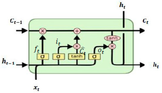
Figure 1.
The structure of Long-Short-Term Memory (LSTM) cells.
3.3. Statistical Components
Statistics is a variable used to analyze and test data in statistical theory. It is the macro performance of data in the statistical domain. This paper creatively applied statistical components as one of the dual channels in the deep model to extract more features. The input matrix of raw time series we already defined as Equation (2). Each raw sample corresponds to six tuples named stics, which contains , , , standard deviation (), skewness (), and kurtosis (), which are defined as Equations (13)–(18).
4. Proposed Deep Model
We propose a deep model that has dual-channel inputs. One is raw data, and the other contains the six tuples of statistical components as we defined above. The overall architecture of the proposed deep model for electricity consumption forecasting can be seen from Figure 2 and a detailed configuration of the proposed deep model is shown in Table 2.
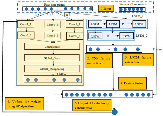
Figure 2.
The architecture of the proposed multi-channels and scales convolutional neural networks (MCSCNN)–LSTM at three levels.
Table 2.
Detailed configuration information of the proposed deep model.
Modifying the hyperparameters such as number and size of filter can improve the performance of the model. We defined the configuration information of MCSCNN–LSTM empirically. Here, we defined as 24. The filter numbers of CNN decrease from 16 to 10 due to the shallow CNN layer being in charge of the detailed local feature extraction; the deeper CNN layer functions to capture abstract global feature representations. At the same time, LSTM is relatively time-consuming, so we defined proper output nodes in two LSTM layers as 20 and 10, respectively. From Figure 2, we can see six parts in our MCSCNN–LSTM: Input, CNN feature extraction, LSTM feature extraction, feature fusion, output, and weights updating. Every part is explained in detail as follows.
4.1. Input
The proposed deep model has double-channel inputs: raw sample from the input matrix and six statistic components , which can be written as:
Moreover, we transform the raw sample into one tensor with the shape of (24, 1), and six tuples stics into tensor with the shape of (6, 1) to satisfy the input requirements of the deep model. The reshaped tensor is defined in (20).
4.2. CNN Feature Extraction
Different from other CNNs, we adopted only one pooling layer to reduce the dimension of extracted features due to the data we used with lees dimensions, which is motivated by [31]. Firstly, CNN models the multi-scale local features from raw sample tensor at three-scale convolution operations—Conv1_1, Conv1_2, and Conv1_3—using different size kernels with shapes of , , . The convoluted results are activated by “ReLU”, as defined in Equation (5). In order to obtain more robust features, we applied one more convolutional layer to extract the abstract feature representations again; they are Conv2_1, Conv2_2, and Conv2_3. At last, extracted multi-local features are processed by one wide convolution layer “Global_Conv” to obtain global representations. CNN extracted features are expressed as Equation (21) and then are flattened for the next step, where is the process of this sub-section.
4.3. LSTM Feature Extraction
Although CNN extracted rich feature representations, we doubt whether CNN can extract some critical hidden features having a long-time dependency. Based on this point, we employed LSTM to extract those features. Two-stacked LSTM layers are employed in this deep model, and every LSTM layer contains some LSTM cells as shown in Figure 1. The features LSTM extracted are expressed as Equation (22). is the process of this sub-section.
4.4. Feature Fusion
Conventional CNN–LSTM is a stacked structure, in which CNN extracted features are processed by LSTM again. Different from conventional CNN–LSTM, this paper adopted a parallel pattern of CNN–LSTM to extract the features and then merged the features they extracted with flattening statistics components. Therefore, we obtained fusion features that are multi-scale and multi-domain (time and statistic domains), which are expressed as:
4.5. Output
After obtaining the rich, robust feature representations, the output is given by using one full connection layer between the output nodes and the fusion features, which can be defined as:
where is the weight matrix and is the bias. This paper mainly focuses on power consumption forecasting of one duration unit (hourly, daily, weekly, and monthly). It is easy to extend the forecast of multi-duration units by setting the nodes of output; we will discuss this later.
4.6. Updating the Networks
Backpropagation [32] algorithm was employed for updating the weights of the hidden layer according to the loss function, and “Adam” [33] was selected as the optimizer for finding the convergence path. The loss function we applied in this deep model is Mean Squared Error (MSE) as shown in Equation (25), where is ground truth electricity consumption and is forecasting electricity consumption using the proposed hybrid deep model.
Electricity forecasting using the proposed model is formalized as Equation (26), where is our model, and is new history electricity consumption data points.
5. Experiment Verification
In order to verify the effectiveness of the proposed deep model, we designed the following experiments using three datasets. The experiments are based on the operating system of Ubuntu 16.04.3, 64 bits with 23.4 GB RAM, and Intel (R) i7-700 CPU of processing speed 3.6 GHz. We used Keras to implement our proposed deep model.
5.1. Dataset Introduction
The data we adopted for validating the priority of the proposed method is from Pennsylvania-New Jersey-Maryland (PJM), which is a regional transmission organization in the USA. It is a part of the Eastern Interconnection grid operating an electric transmission system serving all or parts of some states. Different companies supply different regions. This paper applies three data sets from three companies: American Electric Power (AEP), Commonwealth Edison (COMED), and Dayton Power and Light Company (DAYTON). The raw data set of those is hourly consumption in megawatts (MW), and detailed information is described in Table 3. The data is available on the website of kaggle.com/robikscube/hourly-energy-consumption.
Table 3.
Induction of data sets.
The original data is utilized to validate the effectiveness of VSTF. For the other forecasting tasks, we use an overlapping sample algorithm to generate corresponding samples for each forecast, as shown in Algorithm 1. The stride of the algorithm we defined is one. Notably, we adopted the sample rate of 24 h, 168 h, and 720 h to generate each type of sample for STF, MTF, and LTF. One electricity consumption at different durations is given in Figure 3, in which different types fluctuate differently, respectively, VSTF and STF, which fluctuate frequently.
| Algorithm 1: Overlapping sample algorithm |
| Input: Hourly electricity consumption historical time series Output: Daily, weekly, and monthly electricity consumption historical time series samples and labels. Define the length of samples as 24. Step 1: Integrating the original data for different forecasts #adopt the sample rate of 24 h for STF #adopt the sample rate of 168 h for MTF #adopt the sample rate of 720 h for LTF Step 2: Generating the feature and label of each sample corresponding to the (2) and (3) For in range (): # different forecasts have different contents End for Return , , , , , |
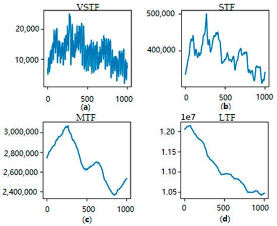
Figure 3.
The electricity consumption at different durations. (a) Hourly electricity consumption for VSTF. (b) Daily electricity consumption for STF. (c) Weekly electricity consumption for MTF. (d) Monthly electricity consumption for LTF.
A description of each data for different forecasts is shown in Table 4. The first 80% of samples are utilized for training the model; the last 20% of samples are utilized to validate. Before starting the experiment, we adopted Equation (27) to normalize each data to work out the impact of different sizes of units, where is the normalized data point of time series and is the raw data sample.
Table 4.
The description of each data set for different forecasts.
5.2. Evaluation Metrics
In order to fairly evaluate the effectiveness of the proposed MCSCNN–LSTM deep model, we adopted multiple evaluation metrics consisting of the root mean square error (RMSE), mean absolute error (MAE), and mean absolute percentage error (MAPE), as shown in Equations (28)–(30), where is the number of testing samples, the is the forecasted value, and is the ground truth. RMSE evaluates the model by the standard deviation of the residuals between real values and forecasted values; MAE is the average vertical distance between ground truth values and forecasted values and is more robust to the larger errors than RMSE. However, when massive data are utilized for training and evaluating the model, the RMSE and MAE increase significantly and quickly. Therefore, MAPE is needed, which is the ratio between residuals and actual values.
5.3. Performance Comparison with Other Excellent Methods
We compared our proposed method to other excellent deep learning-based methods: DNN- [34], NPCNN- [35], LSTM- [20], and CNN–LSTM-based [25] methods. The structure and configuration information of the above comparative methods are given in Table 5. Because the abovementioned methods employed other additional sensor data, we adopted the structure of them only. Conv1D is a convolutional layer with 1-D; Max1D is a max-pooling layer with 1D. We run 10 times of each deep learning-based method to overcome the impact of randomness, and every time runs at 50 epochs. Furthermore, we found the above NPCNN- [35], LSTM- [20], and CNN–LSTM-based [25] methods did not learn at some iterations. It means the loss does not decrease with the increase of training epochs. Instead, they keep one constant value from the first epoch. In summary, NPCNN, LSTM, and CNN–LSTM highly rely on initial processing. The results of this phenomenon are listed in Table 6, which gives the times of the above cases during 10-time training processes for each forecast. Notably, the term “None” means it always learns from raw data and is not sensitive to the random initial settings. For electricity consumption, we must avoid unpredicted and unexpected factors. However, NPCNN- [35], LSTM- [20], and CNN–LSTM-based [25] methods highly rely on initialization. The findings show only DNN [34], and the proposed method always learns so that they are considered as stable.
Table 5.
The structure and configuration information of comparative methods.
Table 6.
The non-training times of each deep learning-based method among 10 times.
We compared the proposed method to the stable DNN [34] with averaged metrics of 10 times, and also compared averaged metrics of the proposed approach to the best results of three unstable methods: NPCNN [35], LSTM [20], and CNN–LSTM [25] in 10 times, as shown in Table 7 with RMSE, Table 8 with MAE, and Table 9 with MAPE. The findings reveal that our proposed method has absolute priority for different durations electricity forecasting at all evaluation metrics compared to DNN. Even when compared to the best results of the other three methods, the proposed MCSCNN–LSTM keeps the highest performance of all metrics for all data sets except for VSTF on the data set DAYTON with evaluation metric MAPE, and RMSE on data set AEP for STF. LSTM [20] performs a little better. In summary, the proposed MSCSNN–LSTM could forecast the electricity consumption of different durations accurately and stably.
Table 7.
The comparison results with RMSE.
Table 8.
The comparison results with MAE.
Table 9.
The comparison results with MAPE.
The averaged improvements of MAPE on different data as shown in Figure 4. The results show that it improves a lot at all durations forecasts. Especially for STF, MTF, and LTF, which was beyond 50% compared to all the above methods. We select stable DNN as listed in Table 7 to compare the predicted results, as shown in Figure 5. The findings show both the proposed method and DNN [34] can predict the global trend of electricity consumption at VSTF, STF, and LTF. However, DNN cannot predict long-term electricity consumption. Moreover, the proposed method outperforms DNN; it can predict more detailed irregular trends for VSTF, STF, and LTF, respectively. We can see details from the marked deep-red box in VSTF and STF of Figure 5.
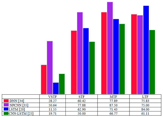
Figure 4.
The averaged MAPE improvement results for each duration forecast compared to other excellent deep learning-based methods on three data sets. Each data set contributes the same to the final outputs.
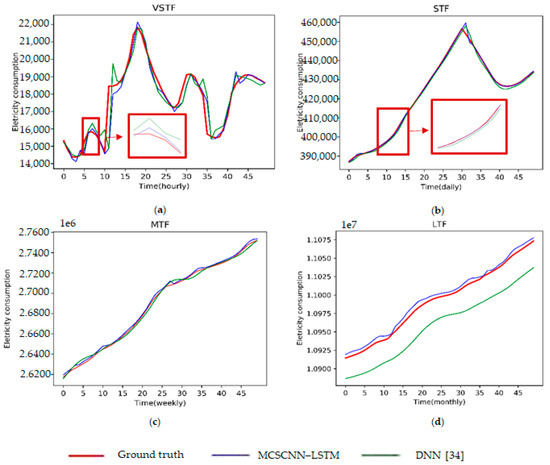
Figure 5.
The comparative forecasting results using two different deep learning-based methods. The x-axis is the time stamp at different duration; the y-axis is electricity consumption. (a) VSTF (hourly) forecasting results. (b) STF (daily) forecasting results. (c) MTF (weekly) forecasting results. (d) LTF (monthly) forecasting results.
5.4. Feature Extraction Capacity of MCSCNN–LSTM
To better understand the feature extraction capacity of the proposed MCSCNN–LSTM, firstly, we compared it to some single models in MCSCNN–LSTM using the metric of MAPE: Multi-Scale CNN (MSCNN), Multi-Channel and Multi-Scale CNN (MCSCNN), and hybrid conventional stacked CNN–LSTM (SCNN–LSTM). The structure of LSTM is the same as [20], which is not stable. All configurations of those models are the same as MCSCNN–LSTM. The results are average of 10 times as shown in Table 10.
Table 10.
The comparison results for validating the feature learning capacity using averaged MAPE.
Comparing the MSCNN with the NPCNN [35], we find that the proposed MSCNN is more stable than general CNN-based methods. The results indicate MSCNN with single input cannot extract satisfactory feature representations for different forecasts of electricity consumption by comparing MSCNN with MCSCNN, especially for STF, MTF, and LTF. By comparing SCNN–LSTM to LSTM, we can see the MCSCNN can extract elegant, robust features to avoid instability and improve performance. We computed the averaged improvement of MAPE on three data sets for different duration forecasts, as shown in Figure 6. MSCNN is selected as the baseline. The findings reveal that the proposed method promotes a lot for all kinds of forecasts. Attentively, the results show only the performance of the MCSCNN on data AEP for VSTF decreased. Furthermore, the level of feature extraction capacity is ranked as proposed: > SCNN–LSTM > MCSCNN > MSCNN.
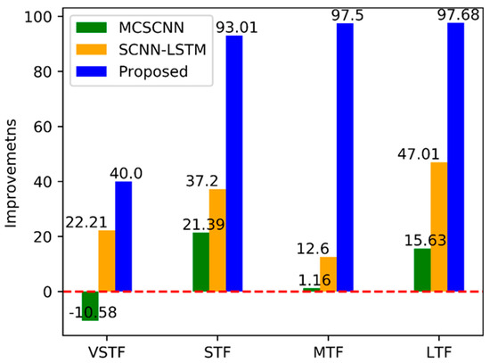
Figure 6.
The averaged improvement of the proposed deep model for each duration forecast based on MSCNN on three data sets.
Secondly, we have analyzed the inside features to confirm the productive feature extraction capacity of the proposed deep model. The visualization results using one VSTF sample shown in Figure 7a,b intimate double-channel inputs: one raw data sample and corresponding statistics components by using the normalized data sample of AEP. Figure 7c is a CNN-learned feature map through the raw data sample. Figure 7d is the feature map of LSTM and we marked it with a red box at the comprehensive feature map Figure 7f, and Figure 7e is a statistic feature map that is marked with the yellow box in Figure 7f. The unmarked part in Figure 7f is a CNN-learned feature map. Figure 7f is a comprehensive feature map. The findings reveal that CNN can learn multi-scale robust global features with less noise because it almost has no changes around 0. The feature map of LSTM ranges from −0.100 to 0.075, and the statistic feature map ranges from 0.00 to 1.75, which indicates statistic components are more useful to extract detailed patterns than LSTM. The comprehensive feature maps combined robust multi-scale global features and detailed features of different domains.
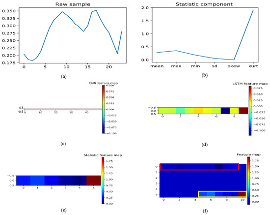
Figure 7.
Feature maps visualization. Each part of the proposed deep model extracted different features. (a) The raw sample channel. (b) The statistic components channel. (c) CNN-learned feature map, which almost has no changes around 0. (d) LSTM-learned feature map, which ranges from –0.10 to 0.075. (e) Statistic components feature map of a reshaped tensor. The raw statistic components channel was reshaped into [1,6], which ranges from 0.00 to 1.75. (f) Reshaped comprehensive feature map. The shape of the obtained feature is 1 by 66, and we reshaped it into 11 by 6 to clearly see and analyze.
5.5. Transfer Learning Capacity Test
We have validated the transfer learning capacity of the proposed method to satisfy the needs in the real-life. For instance, one new company wants to predict electricity consumption, but they do not have enough historical data to train the model. It requires the model with an excellent transfer learning capacity. The following experiments are designed to test the transfer learning capacity of the proposed method, as described in Table 11. We adopted the training part of AEP as the training set to train the model for VSTF, the training part of COMED to train the model for STF, and the training part of DAYTON to train the model for MTF and LTF. The testing part of others is utilized to test.
Table 11.
Experiment design for transfer learning capacity test of the proposed deep model.
The DNN [34] and the proposed MCSCNN–LSTM applied the same data to train and test are considered as comparative experiments to validate the transfer learning capacity. For example, we trained DNN and MCSCNN–LSTM with the training part of COMED, DAYTON, and tested on the testing part of the same data set for VSTF. The results as shown in Figure 8; the x-axis is the testing part of each data set. The results indicate the proposed method has a functional transfer learning capacity, which outperforms DNN [34] for all kinds of forecasts, and a little lower than the proposed method using the same data to train and test the model. We performed a t-test to quantify this difference. The results of the p-value are shown in Table 12. If a p-value is higher than 0.05, it means there is no significant difference. The results show there was no significant difference when we utilized different companies’ data for training the model. Moreover, even though DNN [34] employed the same source data to train and test model, its performance is worse than “transfer”. Notably, there is a significant improvement for the VSTF of electricity consumption compared to DNN. In summary, Figure 8 and Table 12 confirmed that the proposed method has an excellent transfer learning capacity against noisy data.
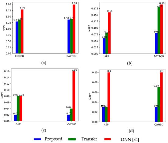
Figure 8.
The average MAPE of different methods to validate the transfer learning capacity of the proposed MCSCNN–LSTM for different forecasts. (a) Transfer learning capacity test for VSTF. (b) Transfer learning capacity test for STF. (c) Transfer learning capacity test for MTF. (d) Transfer learning capacity test for LTF.
Table 12.
The p-value of significance test using t-test.
5.6. Multi-Step Forecasting Capacity Test
Accurate one-step forecasting enables decision-makers to create proper policies and measures of the power supply before one duration. Multi-step forecasting can provide multi-step future consumption information in advance. To validate the multi-step forecasting capacity of the proposed method for multiple forecasts, we designed a five-step forecasting experiment and compared it to [27], which tests the multi-step forecasting capacity of their model for VSTF. The input of the proposed MCSCNN–LSTM for multi-step forecasting in Figure 2 has the same shape with one-step forecasting, we only need to change the output into one vector with five elements regarding the five future consumption data points of each forecast. The comparative results using averaged RMSE, MAE, and MAPE of 10 times are shown in Table 13. AEP is adopted for VSTF and LTF; COMED and DAYTON are adopted for STF and MTF. The results indicate the proposed MCSCNN–LSTM performs very well for STF, MTF, and LTF. Especially, the performance of MTF and LTF has increased tenfold compared to the method of [27] using RMSE, MAE, and MAPE. Only the VSTF is a little worse than [27], but they still are the same level. We also give one sample of five-step forecasting of different forecasts as shown in Figure 9. We can see the proposed MCSCNN–LSTM accurately predicts all types of trends from the raw data and it outperforms [27] CNN–LSTM in terms of handing details. Notably, the proposed method has an absolute advantage in terms of STF, MTF, and LTF.
Table 13.
The multi-step forecasting capacity test results.
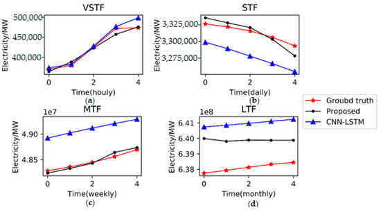
Figure 9.
A comparison of the results of the five-step forecasting using the proposed method and CNN–LSTM [27]. The results indicate the proposed method has an absolute advantage in terms of STF, MTF, and LTF. For VSTF, CNN–LSTM performs a little better than proposed MCSCNN–LSTM. (a) Five-step electricity forecasting results for VSTF. (b) Five-step electricity forecasting results for STF. (c) Five-step electricity forecasting results for MTF. (d) Five-step electricity forecasting results for LTF.
6. Discussion
We have proposed a novel MCSCNN–LSTM that models different domain and multi-scale feature patterns to forecast the electricity consumption at different durations. The difficulty of feature extraction for different durations forecasts using one model, and different duration electricity consumptions have different patterns of the trend as shown in Figure 3, which requires a model with excellent feature extraction capacity with good robustness. Besides, collecting related data such as weather, the temperature is costly and time-consumption. Therefore, we developed MCSCNN–LSTM to extract multi-scale and multi-domain features by only inputting the electricity history data, as shown in Figure 2. We connected CNN and LSTM parallelly with dual inputs, Table 10 and Figure 6 shows it is more effective than conventional stacked CNN–LSTM.
We compared our proposed deep model with other excellent deep models in Table 6, which indicates our proposed model is stable. Furthermore, Table 7, Table 8 and Table 9 and Figure 4 show that we have improved the performance compared to the stable DNN [34] and the best results of NPCNN [35], LSTM [20], and CNN–LSTM [25]. Primarily, it has improved a lot for STF, MTF, and LTF. Figure 5 explained that the proposed method could predict the detailed irregular patterns of electricity consumption.
As can be seen from Table 10, we have analyzed the feature capacity of each part of the proposed MCSCNN–LSTM by comparing the averaged MAPE. In addition, we computed the averaged improvement ratio of the proposed MCSCNN–LSTM by using MCSCNN as the benchmark in Figure 6. It proved that each part of our proposed model has excellent feature extraction capacity. Moreover, we have analyzed the inside feature map of MCSCNN–LSTM as shown in Figure 7, it shows the CNN part of MCSCNN–LSTM can extract multi-scale robust global features, and statistic components are more effective in extracting detailed patterns than LSTM.
As shown in Figure 8, we have designed comparative experiments on three data sets to validate the transfer learning capacity of the proposed MCSCNN–LSTM. The findings from Figure 8 have proven that our proposed deep model has excellent transfer learning skills. In order to quantify the transfer learning capacity, we compared the p-value of the t-test with none-transfer learning methods in Table 12. Moreover, we have confirmed the proposed method could accurately forecast multi-step electricity consumption in advance in Table 13 and Figure 9, the results from Table 13 and Figure 9 indicate our proposed method outperforms CNN–LSTM which was developed in [27].
7. Conclusions
In conclusion, we proposed a novel MCSCNN–LSTM to forecast the electricity consumption at different durations accurately and robustly only by using the self-history data. The comparative analysis has shown that the proposed hybrid deep model MCSCNN–LSTM reaches state-of-the-art performance. The proposed model is compared to other excellent deep learning-based methods to confirm the efficiency and robustness. We run ten times for each model on three data sets to evaluate fairly. The results indicate that our proposed deep model is not sensitive to the initial settings and stable. We compare the forecasted results with other methods to prove that the proposed method can extract more detailed patterns. We also confirmed the necessity of each part in the proposed deep model by comparing the MAPE of each part for electricity forecasting at different durations. We proved that the parallel structure of CNN–LSTM is more potent than conventional stacked CNN–LSTM. We also analyzed the internal feature maps to confirm the feature extraction capacity of each part, and the results show CNN can extract global features; LSTM, and statistic components are in charge of detailed pattern extraction. Some individual experimental cases are designed to validate their excellent transfer learning capacity. We confirmed the proposed MCSCNN–LSTM has excellent multi-step forecasting capacity for STF, MTF, and LTF, respectively. The proposed MCSCNN–LSTM can accurately and stably predict the irregular patterns of electricity consumption at different durations by only using self-history data and have a good transfer learning capacity, which can be easy to extend to other forecasting tasks.
In this paper, we designed the networks empirically. Setting proper hyperparameters can effectively improve forecasting performance. In the feature, we will use deep reinforcement learning to automatically build the model and choose the better hyperparameters of MCSCNN–LSTM for electricity consumption forecasting.
Author Contributions
Designed algorithm, X.S. and C.-S.K.; Performed simulations, X.S.; Preprocessed and analyzed the data X.S. and P.S.; Wrote the paper, X.S.; Provide ideas to improve the performance of algorithm, X.S. and C.-S.K. All authors have read and agreed to the published version of the manuscript.
Funding
This work was supported by the Technology Innovation Program (20004205, The development of smart collaboration manufacturing innovation service platform in textile industry by producer-buyer B2B connection funded By the Ministry of Trade, Industry & Energy (MOTIE, Korea)).
Conflicts of Interest
The authors declare no conflicts of interest.
References
- Ahmad, A.S.; Hassan, M.Y.; Abdullah, M.P.; Rahman, H.A.; Hussin, F.; Abdullah, H.; Saidur, R. A review on applications of ANN and SVM for building electrical energy consumption forecasting. Renew. Sustain. Energy Rev. 2014, 33, 102–109. [Google Scholar] [CrossRef]
- Ayoub, N.; Musharavati, F.; Pokharel, S.; Gabbar, H.A. ANN Model for Energy Demand and Supply Forecasting in a Hybrid Energy Supply System. In Proceedings of the 2018 IEEE International Conference on Smart Energy Grid Engineering (SEGE), Oshawa, ON, Canada, 12–15 August 2018. [Google Scholar]
- Weng, Y.; Wang, X.; Hua, J.; Wang, H.; Kang, M.; Wang, F.Y. Forecasting Horticultural Products Price Using ARIMA Model and Neural Network Based on a Large-Scale Data Set Collected by Web Crawler. IEEE Trans. Comput. Soc. Syst. 2019, 6, 547–553. [Google Scholar] [CrossRef]
- Tang, N.; Mao, S.; Wang, Y.; Nelms, R.M. Solar Power Generation Forecasting With a LASSO-Based Approach. IEEE Internet Things J. 2018, 5, 1090–1099. [Google Scholar] [CrossRef]
- Yu, J.; Lee, H.; Jeong, Y.; Kim, S. Short-term hourly load forecasting using PSO-based AR model. In Proceedings of the 2014 Joint 7th International Conference on Soft Computing and Intelligent Systems (SCIS) and 15th International Symposium on Advanced Intelligent Systems (ISIS), Kitakyushu, Japan, 3–6 December 2014; pp. 1449–1453. [Google Scholar]
- Wu, H.; Wu, H.; Zhu, M.; Chen, W.; Chen, W. A new method of large-scale short-term forecasting of agricultural commodity prices: Illustrated by the case of agricultural markets in Beijing. J. Big Data 2017, 4, 1–22. [Google Scholar] [CrossRef]
- Radziukynas, V.; Klementavicius, A. Short-term wind speed forecasting with ARIMA model. In Proceedings of the 2014 55th International Scientific Conference on Power and Electrical Engineering of Riga Technical University (RTUCON), Riga, Latvia, 14 October 2014; pp. 145–149. [Google Scholar]
- He, H.; Liu, T.; Chen, R.; Xiao, Y.; Yang, J. High frequency short-term demand forecasting model for distribution power grid based on ARIMA. In Proceedings of the 2012 IEEE International Conference on Computer Science and Automation Engineering (CSAE), Zhangjiajie, China, 25–27 May 2012; pp. 293–297. [Google Scholar]
- Mitkov, A.; Noorzad, N.; Gabrovska-Evstatieva, K.; Mihailov, N. Forecasting the energy consumption in Afghanistan with the ARIMA model. In Proceedings of the 2019 16th Conference on Electrical Machines, Drives and Power Systems (ELMA), Varna, Bulgaria, 6–8 June 2019; pp. 1–4. [Google Scholar]
- Jha, G.K.; Sinha, K. Agricultural Price Forecasting Using Neural Network Model: An Innovative Information Delivery System. Agric. Econ. Res. Rev. 2013, 26, 229–239. [Google Scholar] [CrossRef]
- Lecun, Y.; Bengio, Y.; Hinton, G. Deep learning. Nature 2015, 521, 436–444. [Google Scholar] [CrossRef]
- Li, L.; Ota, K.; Dong, M. Everything is image: CNN-based short-term electrical load forecasting for smart grid. In Proceedings of the 2017 14th International Symposium on Pervasive Systems, Algorithms and Networks & 2017 11th International Conference on Frontier of Computer Science and Technology & 2017 Third International Symposium of Creative Computing (ISPAN-FCST-ISCC), Exeter, UK, 21–23 June 2017; pp. 344–351. [Google Scholar]
- Deng, Z.; Wang, B.; Xu, Y.; Xu, T.; Liu, C.; Zhu, Z. Multi-scale convolutional neural network with time-cognition for multi-step short-Term load forecasting. IEEE Access 2019, 7, 88058–88071. [Google Scholar] [CrossRef]
- Suresh, V.; Janik, P.; Rezmer, J.; Leonowicz, Z. Forecasting solar PV output using convolutional neural networks with a sliding window algorithm. Energies 2020, 13, 723. [Google Scholar] [CrossRef]
- Kim, D.; Hwang, S.W.; Kim, J. Very Short-Term Photovoltaic Power Generation Forecasting with Convolutional Neural Networks. In Proceedings of the 9th International Conference on Information and Communication Technology Convergence (ICTC), Jeju, Koera, 17–18 October 2018; pp. 1310–1312. [Google Scholar]
- Hochreiter, S.; Urgen Schmidhuber, J. Long Shortterm Memory. Neural Comput. 1997, 9, 17351780. [Google Scholar] [CrossRef]
- Ma, Y.; Zhang, Q.; Ding, J.; Wang, Q.; Ma, J. Short Term Load Forecasting Based on iForest-LSTM. In Proceedings of the 2019 14th IEEE Conference on Industrial Electronics and Applications (ICIEA), Xi’an, China, 19–21 June 2019; pp. 2278–2282. [Google Scholar]
- Xiuyun, G.; Ying, W.; Yang, G.; Chengzhi, S.; Wen, X.; Yimiao, Y. Short-term Load Forecasting Model ofGRU Network Based on Deep Learning Framework. In Proceedings of the 2018 2nd IEEE Conference on Energy Internet and Energy System Integration (EI2), Beijing, China, 20–22 October 2018; pp. 1–4. [Google Scholar]
- Yu, Y.; Cao, J.; Zhu, J. An LSTM Short-Term Solar Irradiance Forecasting under Complicated Weather Conditions. IEEE Access 2019, 7, 145651–145666. [Google Scholar] [CrossRef]
- Kong, W.; Dong, Z.Y.; Jia, Y.; Hill, D.J.; Xu, Y.; Zhang, Y. Short-Term Residential Load Forecasting Based on LSTM Recurrent Neural Network. IEEE Trans. Smart Grid 2019, 10, 841–851. [Google Scholar] [CrossRef]
- Agrawal, R.K.; Muchahary, F.; Tripathi, M.M. Long term load forecasting with hourly predictions based on long-short-term-memory networks. In Proceedings of the 2018 IEEE Texas Power and Energy Conference (TPEC), College Station, TX, USA, 8–9 February 2018; pp. 1–6. [Google Scholar]
- Han, L.; Peng, Y.; Li, Y.; Yong, B.; Zhou, Q.; Shu, L. Enhanced deep networks for short-term and medium-term load forecasting. IEEE Access 2019, 7, 4045–4055. [Google Scholar] [CrossRef]
- Zhou, H.; Zhang, Y.; Yang, L.; Liu, Q.; Yan, K.; Du, Y. Short-Term photovoltaic power forecasting based on long short term memory neural network and attention mechanism. IEEE Access 2019, 7, 78063–78074. [Google Scholar] [CrossRef]
- Wang, Z.; Lou, Y. Hydrological time series forecast model based on wavelet de-noising and ARIMA-LSTM. In Proceedings of the 2019 IEEE 3rd Information Technology, Networking, Electronic and Automation Control Conference (ITNEC 2019), Chengdu, China, 15–17 March 2019; pp. 1697–1701. [Google Scholar]
- Kim, T.Y.; Cho, S.B. Predicting residential energy consumption using CNN-LSTM neural networks. Energy 2019, 182, 72–81. [Google Scholar] [CrossRef]
- Hu, P.; Tong, J.; Wang, J.; Yang, Y.; Oliveira Turci, L. De A hybrid model based on CNN and Bi-LSTM for urban water demand prediction. In Proceedings of the 2019 IEEE Congress on Evolutionary Computation (CEC), Wellington, New Zealand, 10–13 June 2019; pp. 1088–1094. [Google Scholar]
- Yan, K.; Wang, X.; Du, Y.; Jin, N.; Huang, H.; Zhou, H. Multi-step short-term power consumption forecasting with a hybrid deep learning strategy. Energies 2018, 11, 3089. [Google Scholar] [CrossRef]
- Yan, K.; Li, W.; Ji, Z.; Qi, M.; Du, Y. A Hybrid LSTM Neural Network for Energy Consumption Forecasting of Individual Households. IEEE Access 2019, 7, 157633–157642. [Google Scholar] [CrossRef]
- Peng, H.K.; Marculescu, R. Multi-scale compositionality: Identifying the compositional structures of Social dynamics using deep learning. PLoS ONE 2015, 10, 1–28. [Google Scholar] [CrossRef]
- Chen, Z.; Li, C.; Sanchez, R. Gearbox Fault Identification and Classification with Convolutional Neural Networks. Shock Vib. 2015, 2015, 390134. [Google Scholar] [CrossRef]
- Wang, K.; Qi, X.; Liu, H. A comparison of day-ahead photovoltaic power forecasting models based on deep learning neural network. Appl. Energy 2019, 251, 113315. [Google Scholar] [CrossRef]
- Gupta, J.N.D.; Sexton, R.S. Comparing backpropagation with a genetic algorithm for neural network training. Omega 1999, 27, 679–684. [Google Scholar] [CrossRef]
- Kingma, D.P.; Ba, J.L. Adam: A method for stochastic optimization. In Proceedings of the 3rd International Conference on Learning Representations, ICLR 2015—Conference Track Proceedings, San Diego, CA, USA, 7–9 May 2015; pp. 1–15. [Google Scholar]
- Hu, Q.; Zhang, R.; Zhou, Y. Transfer learning for short-term wind speed prediction with deep neural networks. Renew. Energy 2016, 85, 83–95. [Google Scholar] [CrossRef]
- Liu, S.; Ji, H.; Wang, M.C. Nonpooling Convolutional Neural Network Forecasting for Seasonal Time Series With Trends. IEEE Trans. Neural Netw. Learn. Syst. 2019, 1–10. [Google Scholar] [CrossRef] [PubMed]


© 2020 by the authors. Licensee MDPI, Basel, Switzerland. This article is an open access article distributed under the terms and conditions of the Creative Commons Attribution (CC BY) license (http://creativecommons.org/licenses/by/4.0/).