Article

A Hybrid Time Integration Scheme for the Discontinuous Galerkin Discretizations of Convection-Dominated Problems

School of Aeronautic Science and Engineering, Beihang University, Beijing 100191, China
*
Author to whom correspondence should be addressed.
Energies 2020, 13(8), 1870; https://doi.org/10.3390/en13081870
Submission received: 27 February 2020 / Revised: 29 March 2020 / Accepted: 5 April 2020 / Published: 11 April 2020

Abstract

:
Discontinuous Galerkin (DG) method is a popular high-order accurate method for solving unsteady convection-dominated problems. After spatially discretizing the problem with the DG method, a time integration scheme is necessary for evolving the result. Owing to the stability-based restriction, the time step for an explicit scheme is limited by the smallest element size within the mesh, making the calculation inefficient. In this paper, a hybrid scheme comprising a three-stage, third-order accurate, and strong stability preserving Runge–Kutta (SSP-RK3) scheme and the three-stage, third-order accurate, L-stable, and diagonally implicit Runge–Kutta (LDIRK3) scheme is proposed. By dealing with the coarse and the refined elements with the explicit and implicit schemes, respectively, the time step for the hybrid scheme is free from the limitation of the smallest element size, making the simulation much more efficient. Numerical tests and comparison studies were made to show the performance of the hybrid scheme.

1. Introduction

The convection-dominated problem plays a key role in fluid dynamics, mass and heat transfer, and many other fields. The discontinuous Galerkin (DG) method has become popular for numerically solving convection-dominated problems mainly due to the attractive features of the method. Firstly, a polynomial is used to locally approximate the solution to the governing equation, allowing the method to easily achieve high-order accuracy on unstructured meshes. Secondly, within the framework of the DG method, an element only communicates with its nearest face neighbors. The compact stencil greatly benefits parallel computation. Thirdly, upwinding is introduced in the DG method using numerical flux. The agreement between the numerical method and the convective nature of the governing equation helps to stabilize the calculation.
In 1973, the DG method was first proposed by Reed and Hill in [1]. During the 1980s and the 1990s, the method was fully developed by Cockburn, Shu, Lin, and Hou in a series of papers [2,3,4,5,6]. In those papers, a method-of-lines approach was used for solving the time-dependent conservation laws. That is, the DG method was used to spatially discretize the governing equation; then, a time integration scheme was used to evolve the result in the time domain. This was followed by many other studies. For a comprehensive review of the approach, the reader is referred to [7] (pp. 97–108) and [8] (pp. 171–188). The former discussed cases where the time integration scheme is explicit; the latter concentrated on the cases where the scheme is implicit.
Both the explicit and the implicit schemes have their pros and cons. In realistic applications, the explicit scheme is easy to implement and the computing cost per time step is small. However, the time step length for the explicit scheme is strongly limited by the stability-based Courant–Friedrichs–Lewy (CFL) condition. Although the CFL restriction for the implicit scheme is rather loose, solving nonlinear equations is inevitable for the implicit scheme, making the coding complex and the computing per time step expensive. Therefore, the explicit scheme has prevailed in the research on unsteady problems, whereas the implicit scheme is applied in solving steady problems.
When the mesh for an unsteady problem contains tiny elements, the choice of the time integration scheme was unclear. On one hand, the available time step for an explicit scheme is limited by the smallest element size. Too small an element leads to too many time steps during the calculation. On the other hand, the accuracy with respect to time matters in solving unsteady problems, forbidding the usage of a too big time step. Without a large time step, the implicit scheme is inefficient.
One natural idea to deal with the issue is blending the two schemes. An intuitive research can be found in [9]. For simulating compressible flows, the authors used the additive Runge–Kutta (ARK) scheme [10] to separately deal with the refined and coarse regions of the mesh. In [11], after spatially discretizing the Maxwell’s equations with the DG method, a combination of the explicit leap-frog scheme and the implicit Crank–Nicolson scheme was used to integrate the result. The region-based hybrid scheme was named “locally implicit scheme” by the authors. In [12], a scheme comprising the Verlet scheme and the implicit Crank–Nicolson scheme was chosen to integrate the DG discretization. An error analysis for the hybrid scheme was conducted within the paper. In [13], a locally implicit DG method was used to solve the Maxwell’s equations. The time integration scheme used therein comprised of the implicit Crank–Nicolson scheme and the explicit leap-frog scheme.
In this paper, we develop a new hybrid time integration scheme comprising two high-order schemes for the evolution of the DG discretization. The explicit scheme is the three-stage, third-order accurate, and strong stability preserving Runge–Kutta (SSP-RK3) scheme [14,15] and the implicit one is the three-stage, third-order accurate, L-stable, and diagonally implicit Runge–Kutta (LDIRK3) scheme [16,17,18]. For the purpose of stabilizing the calculation and minimizing the computing consumption, we propose an element grouping strategy corresponding to the hybrid scheme.
The remainder of the paper is organized as follows: In Section 2, we briefly introduce the DG discretization using a model problem. In Section 3, the hybrid time integration scheme, the element grouping strategy, and the nonlinear-solver-related techniques are introduced. Numerical tests are conducted in Section 4 to illustrate the effectiveness of the hybrid scheme. Concluding remarks are provided in Section 5.

2. DG Discretization

In this section, we introduce DG discretization using a two-dimensional (2D) convection-diffusion problem:
u t + · f = ε Δ u , x Ω , t 0 , u ( 0 , x ) = u 0 ( x ) , u ( t , x ) = b ( t , x ) , x Ω , t 0 .
where u = u ( t , x ) , f = ( f 1 ( u ) , f 2 ( u ) ) is the convective flux, u 0 ( x ) defines the initial condition, b ( t , x ) defines the boundary conditions, and Ω R 2 is a bounded domain with a Lipschitz boundary Ω . For a deeper understanding for the DG discretization, the reader is referred to, e.g., Chapter 4 in [8].
We start by introducing notations. After partitioning Ω into K non-overlapping elements, the gathering of the elements is denoted as T h = { Ω k } . For simplicity, we assume the mesh is conforming and shape-regular. We further assume all elements in T h are triangular. By F h , we denote the gathering of element faces in T h . We say Ω k 1 “neighbors on” Ω k 2 when Ω k 1 Ω k 2 F h . For Ω k T h , Ω k denotes the boundary of the element, n k denotes the unit outward normal vector on Ω k , and h k denotes a characteristic size of the element. The solution space for the DG method is defined as:
S h = w : w L 2 Ω ; w Ω k P N Ω k ; Ω k T h ,
where P N denotes the space of polynomials of degree N . We choose the Lagrange polynomials l i k ( x ) , x Ω k , i = 1 , 2 , , N p , defined on uniformly distributed nodes as the bases of P N Ω k . For a triangular element, N p = ( N + 1 ) ( N + 2 ) / 2 . In addition, l i k ( x ) , i = 1 , 2 , , N p , k = 1 , 2 , , K , form the bases of S h . On Ω k , with w and w + denoting the inner and outer traces of function w, respectively, we denote the jump and mean of w as:
w = w w + , w = 1 2 w + w + .
We approximate the solution of Equation (1) with:
u h = k = 1 K u h k = k = 1 K j = 1 N p u j k ( t ) l j k ( x ) ,
where u h k denotes the local approximation on Ω k . By multiplying the governing equation with a test function l i k ( x ) and integrating by parts on Ω k , we obtain:
Ω k d u h k d t l i k d Ω = C i k + D i k ,
where C i k and D i k are the DG discretizations for the convective item and the diffusive item, respectively [19]. The expression for C i k is:
Ω k f ( u h k ) · l i k d Ω Ω k H ^ l i k d S
where H ^ is the inviscid numerical flux. A popular type is the local Lax–Friedriches (LLF) flux [7] (p. 170):
H ^ = f u · n k + 1 2 λ u ,
where λ is defined as:
λ = max u [ min { u , u + } , max { u , u + } ] n k · f u .
If a face of Ω k coincides with Ω , then the u + on the face is defined using the boundary conditions. An introduction of various inviscid numerical fluxes can be found in [20].
Within the frame of the DG method, different approaches are possible for dealing with the diffusive item: the Bassi–Rebay approach [21], the local DG approach [22], the compact DG approach [23], and the direct DG approach [24]. In our work, we apply the non-symmetric interior penalty Galerkin (NIPG) approach [8] (pp. 37–43). Therefore,
D i k = Ω k ε u h k · l i k d Ω + Ω k ε u h · n k l i k σ u h l i k u h n k · 1 2 l i k d S ,
where the penalty weight σ is defined as:
σ Γ = 1 h Γ , Γ F h .
where h Γ denotes the length of element face Γ . Similar to the case for the convective item, the outer traces on Ω are provided by the boundary conditions.
Formulating Equation (5) using all base functions of S h , we obtain a system of ordinary differential equations (ODEs):
d d t U = M 1 R F ,
where:
U = U 1 U 2 U K , M = M 1 0 0 0 M 2 0 0 0 M K , R = R 1 R 2 R K , F = F 1 F 2 F K .
For Ω k T h :
U k = u 1 k ( t ) u N p k ( t ) , M k = Ω k l 1 k l 1 k d Ω Ω k l N p k l 1 k d Ω Ω k l 1 k l N p k d Ω Ω k l N p k l N p k d Ω ,
R k denotes the right-hand sides of Equation (5) with i ranging from 1 to N p and F k = ( M k ) 1 R k .
In our applications, the spatial integrations are calculated using the Gauss quadrature rule. Specifically, the accuracy orders for the integrations over an element and an element face are 2 N and 2 N + 1 , respectively, with N denoting the degree for the polynomial used for local approximation.

3. Time Integration

3.1. Basic Schemes

Multi-stage Runge–Kutta (RK) schemes are considered in this paper to integrate Equation (11) from time t n to t n + 1 . An s-stage RK scheme has the form [25]:
U ( i ) = U n + Δ t j = 1 s a i j F ( t n + c j Δ t , U ( j ) ) , U n + 1 = U n + Δ t j = 1 s b j F ( t n + c j Δ t , U ( j ) ) ,
where Δ t = t n + 1 t n , U n = U ( t n ) and the coefficients a i j , b j , and c j differ with specific RK schemes. The coefficients for SSP-RK3 and LDIRK3 are given by the following Butcher tableaus:
Energies 13 01870 i001
and
Energies 13 01870 i002
For SSP-RK3, Equation (15) characterizes a i j = 0 , i j . That is, the calculation for the ith stage only requires the data of previous stages. This makes the explicit scheme easy to implement. However, its time step length is severely restricted by the CFL condition. When the DG solution for a d-dimensional time-dependent conservation law is sought from S h , the time step corresponding to SSP-RK3 has to satisfy [3,26]:
Δ t 1 d 1 ( 2 N + 1 ) h k λ k , Ω k T h ,
where λ k is the biggest characteristic velocity on Ω k . A rather small Δ t is required when tiny elements exist in T h , making the simulation less efficient. For LDIRK3, the stability-based restriction on the time step is loose. Its available time step can be hundreds of times bigger than that for an explicit scheme [27]. However, due to the non-zero diagonal coefficients in Equation (16), nonlinear equations have to be solved during the time integration. Taking the first stage of Equation (16) as an example, we need to solve
U ( 1 ) = U n + α Δ t · F ( t n + α Δ t , U ( 1 ) ) ,
to get U ( 1 ) . This is usually achieved with the Newton–Raphson method, i.e.,
J ( U ( 1 ) , m ) Δ U ( 1 ) , m = U n + α Δ t · F ( t n + α Δ t , U ( 1 ) , m ) U ( 1 ) , m , U ( 1 ) , m + 1 = U ( 1 ) , m + Δ U ( 1 ) , m , m = 0 , 1 ,
where the global Jacobian matrix is defined as:
J ( U ( 1 ) , m ) α Δ t · F U ( 1 ) , m I ,
where I is the identity matrix. In solving a scalar problem with the DG method, there are ( N p · K ) 2 values in J . Both the construction of the matrix and the solution of the linear equations, e.g., Equation (19), are computing-expensive and time-consuming. When the nonlinear-solver-related calculation cannot be compensated by a big time step, the implicit scheme is inefficient.

3.2. A New Hybrid Scheme

3.2.1. Elements Grouping and Scheme Coupling

According to their size, the elements in T h are gathered into the explicit set T h , e x and the implicit set T h , i m . Generally, all elements in T h , e x are coarse, whereas all fine elements are collected in T h , i m . An index quantifying the element size variance is defined as [9]:
S = mi n Ω k T h , e x h k mi n Ω k T h , i m h k .
Similar to [9], the ODEs in Equation (11) are divided into two groups:
d d t U e x = F e x , d d t U i m = F i m ,
where U e x and U i m correspond to T h , e x and T h , i m , respectively.
From t n to t n + 1 , the ith stage for an s-stage RK scheme corresponds to t n + c i Δ t , where Δ t = t n + 1 t n and c i can be found in the left row of the Butcher tableau. That is, U ( i ) in Equation (14) can be explained as the numerical solution corresponding to t n + c i Δ t . The ARK scheme developed in [10] consists of an explicit RK scheme, denoted by ARK( e x ), and an implicit RK scheme, denoted by ARK( i m ). Their Butcher tableaus characterize that c i , ARK ( e x ) = c i , ARK ( i m ) , i = 1 , 2 , , s . Therefore, the ith stage of ARK( e x ) and that of ARK( i m ) correspond to the same time, which considerably simplifies the coupling between the two schemes. In [9], for the ith stage of ARK, U e x ( i ) is firstly calculated with the ith stage of ARK( e x ), then U i m ( i ) is calculated with the ith stage of ARK( i m ), using U e x ( i ) as boundary conditions.
In Equations (15) and (16), the coefficients c i , i = 1 , 2 , 3 , for SSP-RK3 and LDIRK3 are different. However, the two ends of the time step are universal for the two schemes. Therefore, our hybrid scheme consists of two phases: achieving U e x ( t n + 1 ) with SSP-RK3 first, then achieving U i m ( t n + 1 ) with LDIRK3.
According to Equation (15), the SSP-RK3 scheme can be written as:
U ( 1 ) = U n , U ( 2 ) = U n + Δ t · F ( t n , U ( 1 ) ) , U ( 3 ) = U n + 1 4 Δ t · F ( t n , U ( 1 ) ) + F ( t n + Δ t , U ( 2 ) ) , U n + 1 = U n + Δ t · 1 6 F ( t n , U ( 1 ) ) + 1 6 F ( t n + Δ t , U ( 2 ) ) + 2 3 F ( t n + 1 2 Δ t , U ( 3 ) ) .
A sketch of a one-dimensional (1D) mesh for the DG method is provided in Figure 1, where the elements around the interface between T h , e x and T h , i m are marked by δ , θ , ζ and η . In the following descriptions, we let the element marker represent the local approximation on the element and omit the time in F , e.g., δ n + 1 denotes U n + 1 ( δ ) and F ( δ ( 1 ) ) denotes F ( t n , U ( 1 ) ( δ ) ) . The elements in T h , i m that are necessary in computing δ n + 1 can be identified using Equation (23).
Theorem 1.
Within time step [ t n , t n + 1 ] , when SSP-RK3 is taken to achieve the local DG solution on a given element, the nearest three layers of elements are involved in the computation.
Proof .
We restrict our discussion to one side of a 1D element for simplicity.
According to Equation (5), when applying the operator F to the local DG approximation on a given element, the local approximations on the face neighbors of the element are involved. In Figure 1, F ( δ ( 1 ) ) involves θ ( 1 ) , F ( θ ( 1 ) ) involves ζ ( 1 ) , F ( ζ ( 1 ) ) involves η ( 1 ) , F ( δ ( 2 ) ) involves θ ( 2 ) , F ( θ ( 2 ) ) involves ζ ( 2 ) , and F ( δ ( 3 ) ) involves θ ( 3 ) .
According to the second line in Equation (23), F ( δ ( 1 ) ) contributes to δ ( 2 ) . Therefore, δ ( 2 ) requires θ ( 1 ) because F ( δ ( 1 ) ) involves θ ( 1 ) . Similarly, θ ( 2 ) requires ζ ( 1 ) .
According to the third line in Equation (23), F ( δ ( 2 ) ) contributes to δ ( 3 ) . Therefore, δ ( 3 ) requires θ ( 2 ) because F ( δ ( 2 ) ) involves θ ( 2 ) . θ ( 2 ) requiring ζ ( 1 ) is already known. Therefore, δ ( 3 ) requires ζ ( 1 ) . Similarly, θ ( 3 ) requires η ( 1 ) .
According to the last line in Equation (23), F ( δ ( 3 ) ) contributes to δ n + 1 . Therefore, δ n + 1 requires θ ( 3 ) because F ( δ ( 3 ) ) involves θ ( 3 ) . θ ( 3 ) requiring η ( 1 ) is already known. Therefore, δ n + 1 requires η ( 1 ) . □
SSP-RK3 depends on the solutions of t n . According to Theorem 1, to achieve a reliable U ex ( t n + 1 ) with SSP-RK3, the t n -approximations on the outer two layers beyond T h , e x , together with the trace value of the outer third layer, must be reliable. In our applications, a region two layers wider than T h , e x is named T h , e x 1 . All elements in T h , e x 1 undergo the SSP-RK3 integration during the explicit phase of the hybrid scheme. Only the solutions corresponding to T h , e x are retained as reliable approximations for t n + 1 .
The calculation of U i m ( t n + 1 ) is straightforward. At the ith stage of LDIRK3, the local approximations of t n + c i , LDIRK 3 Δ t are first achieved using SSP-RK3, providing the boundary conditions for the implicit integration on T h , i m . Here, the region for the SSP-RK3 is denoted by T h , e x 2 . In Figure 1, T h , e x 2 is comprised of five elements centered at δ because only the trace value of U ( t n + c i , LDIRK 3 Δ t , δ ) is useful for the implicit integration on T h , i m .

3.2.2. Constructing the Jacobian Matrix

During the implicit phase of the hybrid scheme, a Newton-type nonlinear solver is necessary. As is shown in Equation (19), the Jacobian matrix is a key to the solver.
Here, we describe an analytic method of constructing the matrix J R R / U , where R and U are defined in Equation (12). There are ( N p × K ) 2 values in J R . Being divided into K 2 squares, the ( m , n )th square, denoted by J R m , n , equals R m / U n . According to Equation (5), J R m , n is full of zeros except for the cases where m = n or Ω m neighbors on Ω n .
We first consider J R m , m . By taking the partial derivative of the right-hand sides of Equation (5) with respect to u j m , the ( i , j )th value in the square is calculated by:
J R m , m ( i , j ) = Ω m f u u h m l j m · l i m d Ω Ω m H ^ u h m l j m l i m d S Ω m ε l j m · l i m d Ω + Ω m ε 1 2 l j m · n m l i m σ l j m l i m l j m n m · 1 2 l i m d S .
For the LLF flux in Equation (7), we take:
H ^ u h m = 1 2 f u u h m · n m + 1 2 λ .
Next, we consider J R m , n where Ω m neighbors on Ω n . By taking the partial derivative of the right-hand sides of Equation (5) with respect to u j n , the ( i , j )th value of the square is calculated as:
J R m , n i , j = Ω m H ^ u h n l j n l i m d S + Ω m ε 1 2 l j n · n m l i m + σ l j n l i m + l j n n m · 1 2 l i m d S ,
where, for the LLF flux,
H ^ u h n = 1 2 f u u h m · n m 1 2 λ .
Within J R , only the portions related to T h , i m are useful to the hybrid scheme. We restrict ourselves to calculating the squares corresponding to T h , i m and leave out the the squares related to T h , e x . This greatly reduces the required time and computing resources.

3.3. Nonlinear Solver

In our applications, an inexact Newton–Raphson method is used for solving the nonlinear equations. That is, within the time step [ t n , t n + 1 ], the Jacobian matrix is computed with the data corresponding to t n , then the matrix is reused in the remaining iterations as well as stages [25]. Without hardly affecting the convergence rate, the inexact method leads to a large reduction in computing expense.
For the purpose of solving the linear equations arising from the inexact Newton–Raphson method, a preconditioned generalized minimal residual (GMRES) method is adopted. The preconditioner is constructed using the incomplete lower-upper (ILU) decomposition method. To further accelerate the convergence of the GMRES method, the reverse Cuthill–Mckee (RCM) algorithm is taken to narrow the difference between the preconditioner and the coefficient matrix for the linear equations. A comprehensive view of the linear solver can be found in, e.g., [28].

3.4. Stability

Here we discuss the regions of absolute stability of the time integrations schemes mentioned above. For the purpose of deciding the region, we apply the scheme to the model ODE:
d u d t = λ u ,
where λ is a complex constant. For RK schemes, the numerical solution corresponding to t n + 1 can be expressed as the product of that corresponding to t n and an increment function, i.e.,
u n + 1 = R ( z ) u n ,
where z λ Δ t and Δ t = t n + 1 t n . A time integration scheme is stable when R ( z ) 1 .
For the SSP-RK3 in Equation (15), the increment function is expressed as:
R ( z ) SSP RK 3 = 1 + z + 1 2 z 2 + 1 6 z 3 .
For the LDIRK3 in Equation (16),
R ( z ) LDIRK 3 = ( α β 1 α 2 + 2 α β 2 β 2 γ ) z 2 + ( 2 α β 1 β 2 ) z 1 ( α z 1 ) 3 ,
where the coefficients α , β 1 , β 2 a n d γ can be found in Equation (16).
In Figure 2 we plot the absolute stability regions for the SSP-RK3 scheme and the LDIRK3 scheme. For the evolution of the ODEs, e.g., Equation (11), the complex constant λ in Equation (28) can be explained as the eigenvalue with the biggest norm of the system. It quantifies the stiffness of the system and is determined by the by the specific way of spatial discretization. In [9], the stiffness portion related to the element size is denoted as “geometry-induced stiffness”. This can be expressed as λ = λ ( h k ) , Ω k T h .
As is shown in Figure 2a, the stability region of SSP-RK3 is bounded by a closed curve. Its time step have to vary with λ , i.e., Δ t = Δ t ( λ ( h k ) ) = Δ t ( h k ) , Ω k T h , to ensure that z λ Δ t lying within the stability region. On the other hand, as is seen in Figure 2b, z , z = belongs to the stability region of LDIRK3, making whose time step free from the affection of λ . In our hybrid scheme, the elements in T h , e x and T h , i m are separately treated with the SSP-RK3 scheme and LDIRK3 scheme. Therefore, its time step is limited by the elements sizes in T h , e x , but free from the element size restriction of T h , i m , i.e., Δ t = Δ t ( h k ) , Ω k T h , e x . To summarize, the time step for our hybrid scheme is decided in such a way that it maintains the stability of SSP-RK3 on T h , e x . Therefore, we believe Figure 2a can be reused to illustrate the stability region of our hybrid scheme, on condition taking in mind that Δ t = Δ t ( h k ) , Ω k T h , e x .

4. Numerical Tests

We execute numerical tests with unsteady problems in this section. All computations are performed on a laptop equipped with an Intel Core 2.6 GHz processor and 6GB memory. For each problem, we apply the hybrid scheme to evolve the DG discretization. In addition, we also integrate the DG discretization with the SSP-RK3 scheme and a four-stage, third-order accurate SSP-RK scheme [29], denoted by SSP-RK3-4, to compare the performances of the schemes in terms of efficiency. In 
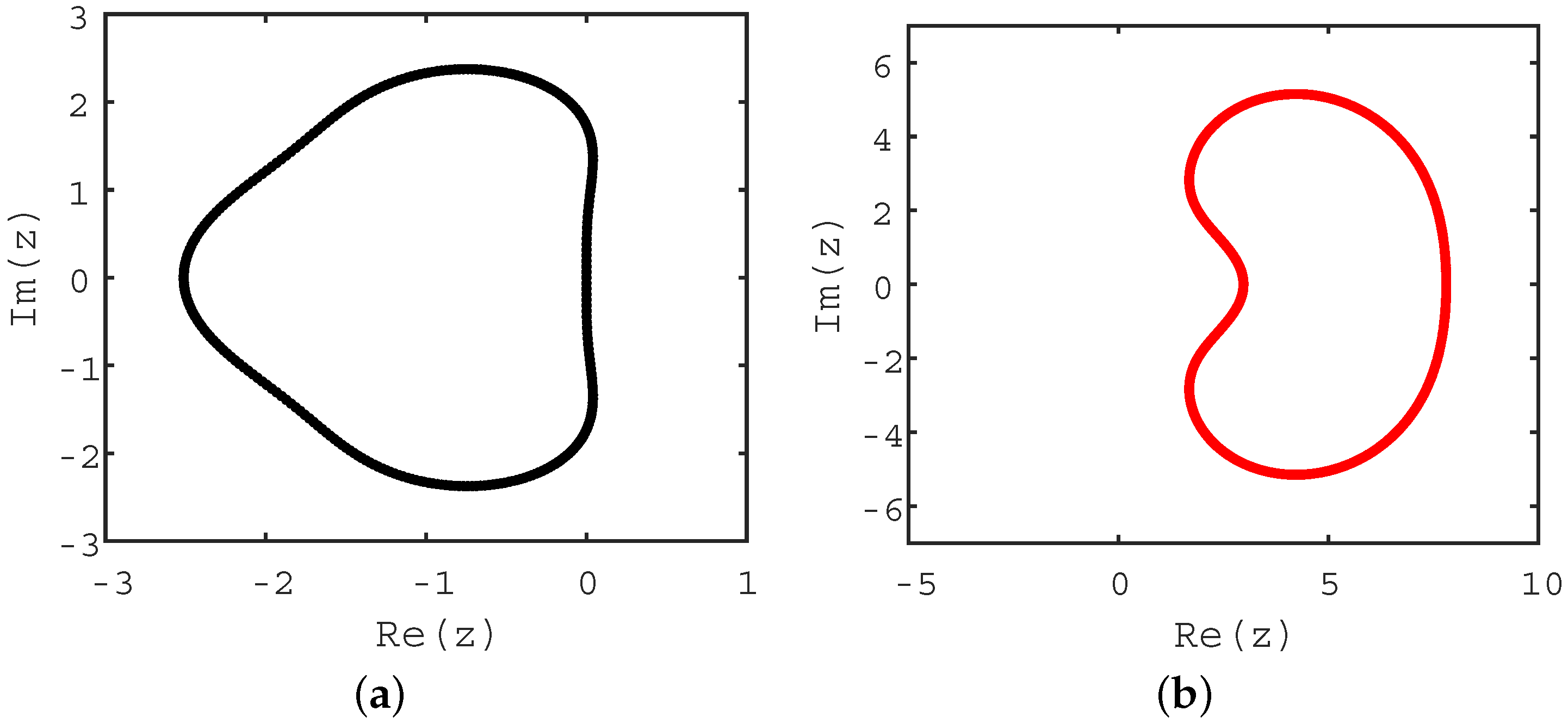
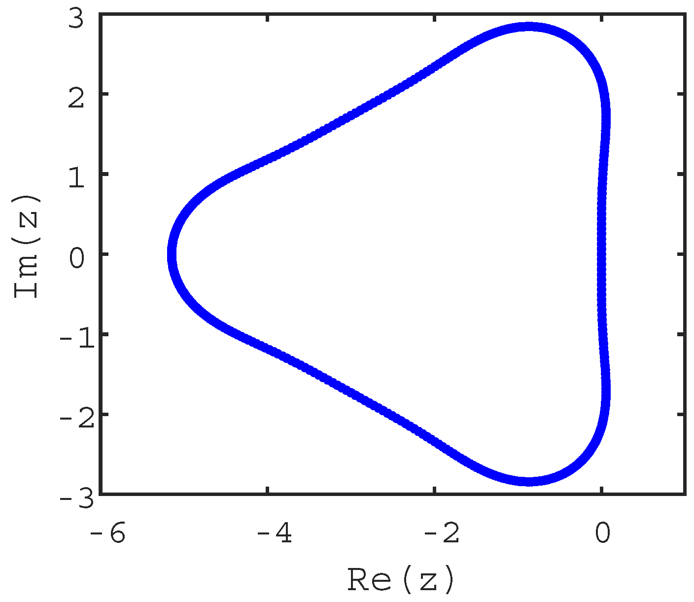
Appendix A, we provide the Butcher tableau of the SSP-RK3-4 scheme and plot its region of absolute stability. Compared with Figure 2a, the stability region for the SSP-RK3-4 scheme is bigger. According to [29], the available CFL number for the SSP-RK3-4 scheme is twice that for the SSP-RK3 scheme.
For our hybrid scheme, the time step length is decided by:
Δ t hybrid = 1 d 1 ( 2 N + 1 ) min Δ t e x , Δ t i m , Δ t e x = C e x · min Ω k T h , e x h k λ k , Δ t i m = C i m · min Ω k T h , i m h k λ k ,
where d denotes the spatial dimension of the problem, h k takes the element length for 1D problems or the inscribed circle diameter of the element in 2D problems, λ k differs with the specific problem, and C e x and C i m are adjustable parameters. We take C i m / C e x S , with S defined in Equation (21). For the SSP-RK3 scheme, the time step is decided by:
Δ t RK 3 = C e x ( 2 N + 1 ) · min Ω k T h h k λ k .
For the SSP-RK3-4 scheme, we set the time step two times as big as that for the SSP-RK3 scheme, i.e.,
Δ t RK 3 4 = 2 Δ t RK 3 .
For problems with analytic solutions, we calculate the L 2 errors of the numerical results. Given the numerical solution, u h , and the analytic solution, u a n a l y , the L 2 error is defined as [30]:
e 2 = k = 1 K Ω k u h u a n a l y 2 d Ω .

4.1. 1D Linear Advection Problem

The problem is governed by:
q t + a q x = 0 , x 1 , 1 , t 0 , q 0 , x = 1 + cos 2 π x ,
and the boundary conditions are periodic. The analytic solution to the problem is q ( t , x ) = 1 + cos ( 2 π ( x a t ) ) .
We numerically solve the problem with a = 1 on three meshes, denoted by “Coarse 1D”, “Middle 1D”, and “Fine 1D”. During the mesh generation, the computational domain is divided into three regions: the left, the central and the right. The left and the right regions are symmetric with respect to the origin. The grids are uniformly distributed in the two regions. The range of the central region is kept four times the element size in the left/right region. In the central region, the grids are symmetrically distributed. The smallest element size in the central region is kept one-tenth of that in the left/right region, resulting in S = 10 . In the central region, the ratio between the adjacent element sizes is kept less than 1.5. The biggest element sizes in Coarse 1D, Middle 1D, and Fine 1D are 0 . 1 , 0 . 05 , and 0 . 025 , respectively.
Here are some remarks on the meshes. Generally the ratio between the adjacent element sizes should not exceed 1.2 in order to avoid big interpolation error. However, in the DG method, the high-order accuracy is achieved by increasing node numbers within the elements. There is no need to expand the stencil, as is done in the finite difference (FD) method or the finite volume (FV) method. In addition, as is shown in Equations (6) and (9), the DG solution is allowed to be discontinuous on element interfaces. The coupling between the local approximations is weak. Therefore, at least for the problems with smooth solutions, we believe the impact of the big element size change is endurable for the DG method. Last but not least, this kind of sudden jump in the size of element also appears in [9]. See Figure 6a therein for reference.
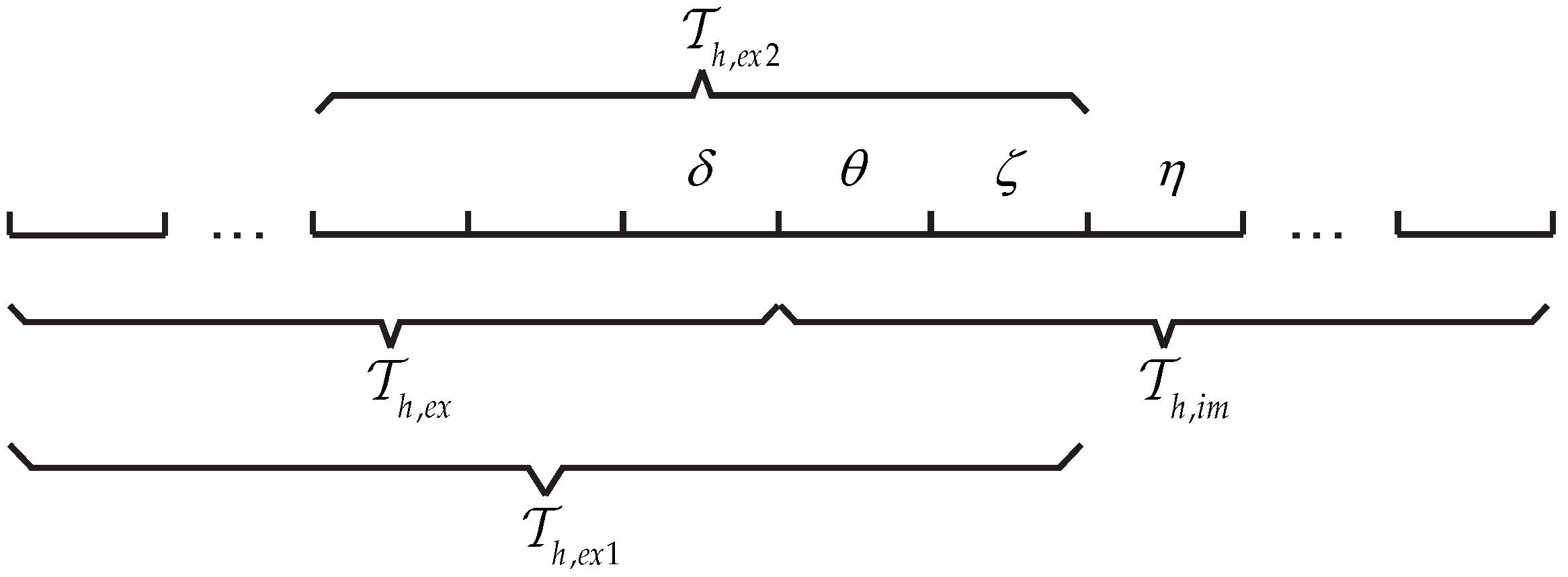
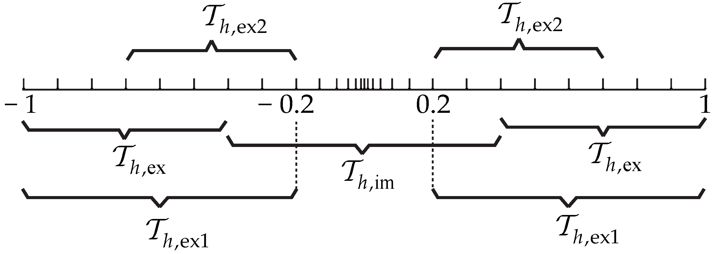
Figure 3 shows the Coarse 1D mesh and its elements grouping. The roles of T h , i m , T h , e x , T h , e x 1 , and T h , e x 2 during the temporal integration are same as in Figure 1. Since the time step is restricted by the elements that subjected to the explicit integration, i.e., the elements in T h , e x 1 , the outer two layers of elements in T h , i m are coarse. The elements groupings for Middle 1D and Fine 1D are similar to that for Coarse 1D.
For each calculation, we take N = 2 for local approximations. We spatially discretize the problem according to Section 2. Since there is no diffusive item in the governing equation, we leave the diffusion-related items in the discretizations as zeros. For deciding the time steps, we take d = 1 , C e x = 1 , C i m = 10 and λ k = a . Each calculation is run up to t = 1 .
Table 1 shows the L 2 error of the numerical result for each mesh and the convergence order of the errors. We found that the convergence order in space is N + 1 , which is optional for the DG method in solving conservation laws [6]. According to [6], to guarantee the domination of the spatial error, the accurate order for the time integration scheme is at least N + 1 . The optional convergence order in Table 1 indicates that the hybrid scheme maintains the high-order accuracy of SSP-RK3 or LDIRK3. It also proves that the big size changes in the mesh has little effect on the accuracy of the method.
Table 2 compares the efficiency of the SSP-RK3 scheme (RK3), the SSP-RK3-4 scheme (RK3-4) and our hybrid scheme (hybrid). The second to the fourth columns show the average time step lengths for different schemes. The fifth to the last columns record the CPU time (in seconds) for the simulations. In accordance with Equations (32)–(34), the average time steps for the SSP-RK3-4 scheme and the hybrid scheme are twice and S times as that for the SSP-RK3 scheme, respectively. On the other hand, the CPU time indicate that the acceleration of the computation does not scale linearly with the amplification of the time step. For the SSP-RK3-4 scheme, this is owing to the computation related to the extra fourth stage. For our hybrid scheme, this may comes from the nonlinear-solver-related calculations, e.g., constructing the Jacobian matrix and solving linear systems. Nevertheless, based on the given meshes, it is clear that the hybrid scheme is superior towards the SSP-RK3 scheme or the SSP-RK3-4 scheme in terms of efficiency.

4.2. 1D Linear Advection-Difussion Problem

The problem is governed by:
q t + a q x = ϵ 2 q x 2 , x 1 , 1 , t 0 , q 0 , x = sin π x .
The analytic solution to the problem is q t , x = exp π 2 ϵ t sin π x a t . The boundary conditions are applied using the analytic solution.
We numerically solve the problem with a = 1 and ϵ = 0 . 01 . The meshes being used are same as in Section 4.1. N = 1 is taken for the local approximations. The spatial discretization for the problem is the same as in Section 2. To find the upper limit of C e m , we first apply the SSP-RK3 scheme. The definition of λ k is given by:
λ k = a + N 2 ϵ h k .
Through numerical tests, we find that the maximum of C e x for maintaining the calculation stability is 0.3. For defining the time step for the hybrid scheme, we take d = 1 , C e x = 0 . 3 , C i m = 3 . Each calculation is run up to t = 0 . 1 .
Table 3 shows the L 2 errors of the numerical results and their convergence order. According to [8] (p. 75), when the NIPG approach is selected for dealing with the diffusive item, the theoretical convergence order measured in L 2 -norm is N + 1 when N is odd. We found that the numerical results matched well with the theory. Table 4 compares the efficiency of different schemes. Similar to the results in Section 4.1, in every simulation, the hybrid scheme enjoyed the biggest available time step and consumed the least CPU time.

4.3. 1D Euler System

The problem is governed by:
q t + f x = 0 , x [ 1 , 1 ] , t 0 ,
where:
q = ρ ρ u E , f = ρ u ρ u 2 + p ( E + p ) u ,
where ρ is the density, u is the velocity, p is the pressure, and E = ρ u 2 / 2 + p / ( γ 1 ) is the total energy. Here γ = 1 . 4 .
We define the initial condition as:
ρ 0 , x = 1 + 0 . 2 sin π x , u 0 , x = 1 , p 0 , x = 1 ,
and apply periodic boundary conditions. The analytic solution to the problem is:
ρ t , x = 1 + 0 . 2 sin π x t , u t , x = 1 , p t , x = 1 .
The meshes being used are same as in Section 4.1. N = 2 is taken for local approximations. During the spatial discretization, the Vijayasundaram flux [31]:
H ^ V i j a ( H ^ 1 , H ^ 2 , H ^ 3 ) T = P q , n k q + P + q , n k q + ,
is chosen as the inviscid numerical flux. The treatment for each equation of the governing system is similar to that in Section 2. In our application, the ODEs pending to the temporal integration are:
d d t Q s y s = M s y s 1 R s y s F s y s ,
where:
Q s y s = Q 1 Q 2 Q 3 , M s y s = M 1 M 2 M 3 , R s y s = R 1 R 2 R 3 , F s y s = F 1 F 2 F 3 ,
where Q e , M e , R e , F e , e = 1 , 2 , 3 , correspond to the eth equation of the governing system. Their definitions are similar to that in Equation (12).
When integrating Equation (44) with the hybrid scheme, it is necessary to construct the matrix J R , s y s R s y s / Q s y s . For the 1D Euler system, J R , s y s consists of 3 × 3 blocks. The calculation for the ( e 1 , e 2 ) th block, i.e., R e 1 / Q e 2 , is similar to that in Section 3.2.2. The matrices P and P + are directly taken as the partial derivatives of H ^ V i j a with respect to q and q + , respectively. For defining time steps using Equations (32)–(34), we take d = 1 , C e m = 1 and C i m = 10 . The definition of λ k is:
λ k = max x Ω k u , u c , u + c ,
where c = γ p / ρ is the speed of sound. Each calculation is run up to t = 0 . 5 .
Table 5 shows the L 2 errors of the densities and their convergence order. We found that the optimal ( N + 1 )th order is well attained. Table 6 compares the available time step lengths and the CPU time for different schemes. Again the hybrid scheme enjoyed the biggest time step and the least CPU time.

4.4. 2D Euler System

The problem is governed by:
q t + f x + g y = 0 , ( x , y ) [ 5 , 5 ] × [ 5 , 5 ] , t 0 ,
where:
q = ρ ρ u ρ v E , f = ρ u ρ u 2 + p ρ u v ( E + p ) u , g = ρ v ρ u v ρ v 2 + p ( E + p ) v .
In Equation (48), ρ is the density, u and v are the velocity components, p is the pressure, and E = ρ ( u 2 + v 2 ) / 2 + p / ( γ 1 ) with γ = 1 . 4 is the total energy. We consider an isentropic vortex problem with the analytic solution [7] (p. 209):
ρ t , x , y = 1 γ 1 16 γ π 2 exp 2 2 x t 2 2 y 2 1 γ 1 , u t , x , y = 1 y 2 π exp 1 x t 2 y 2 , v t , x , y = x 2 π exp 1 x t 2 y 2 , p t , x , y = ρ t , x , y γ .
It is used for defining the initial condition and boundary conditions for numerical simulations.
We solve the problem on three meshes, denoted by “Coarse 2D”, “Middle 2D”, and “Fine 2D”. In each mesh, the domain is divided into the surrounding region and the central region. The coarse elements in the surrounding region are made by diagonalizing the squares of same sizes. The central region is a square whose side length is kept two times the leg length for the coarse element. The elements in the central region are refined artificially. The smallest element length is kept one-eighth of that in the surrounding region, leading to S = 8 . The ratio between the adjacent element sizes is kept less than 1.5 during the refinement. Since all elements within the mesh are are isosceles right triangles, the skewness (measured by the normalized equiangular method) for the mesh is constant 0.25 and the aspect ratio is 1 . 41 . The biggest leg lengths in Coarse 2D, Middle 2D, and Fine 2D are 0.5, 0.25, and 0.125, respectively.
Here are some remarks concerning the quality of the 2D meshes. Similar to the 1D cases, we believe the impact of the radical size change is minimized by the independence of the local approximations in the DG method. In addition, the radical size jump in element size is common in relevant researches, see, e.g., Figure 8 in [9], Figure 5 in [11] and Figure 1c in [12], for reference.
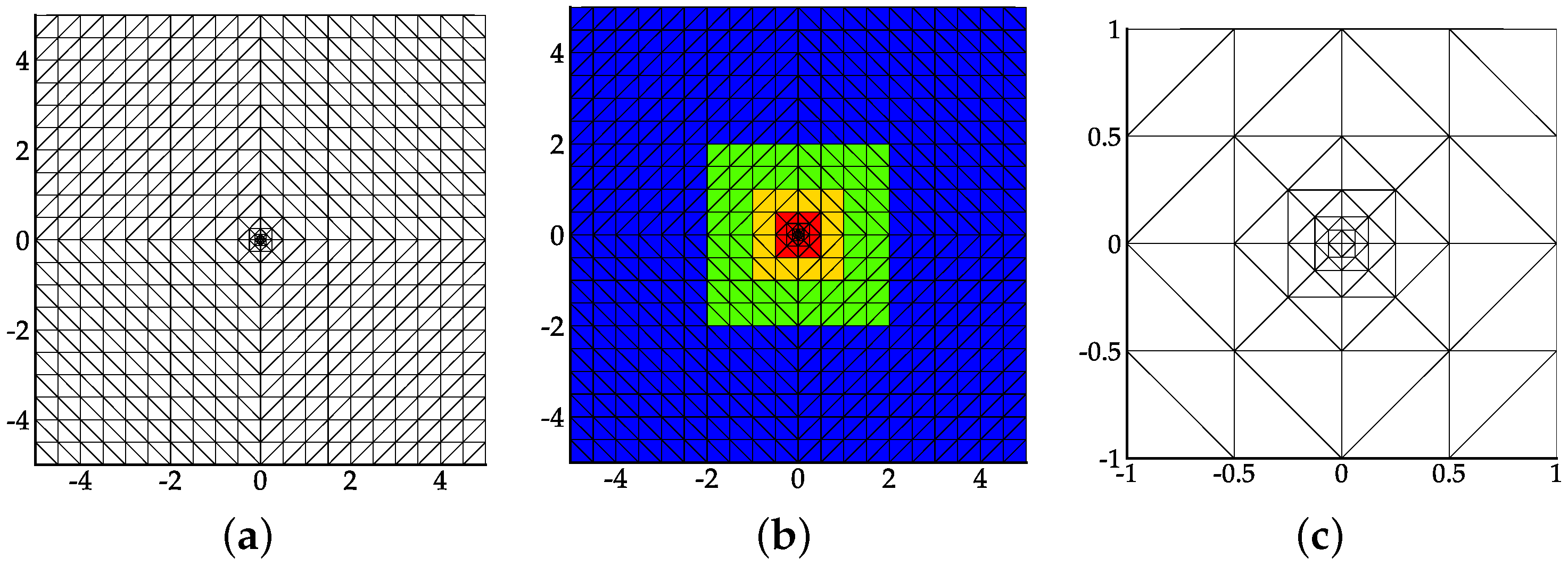
Figure 4 shows the Coarse 2D mesh and its elements grouping. The grouping strategy for the 2D elements is similar to the 1D case. The relationship between the color and the membership for an element is given in Table 7. The elements groupings for Middle 2D and Fine 2D are similar to that for Coarse 2D.
For each calculation, N = 2 is taken for local approximations. The spatial discretization for the problem is similar to that in Section 4.3. For defining time steps, we take d = 2 , C e x = 1 and C i m = 8 . The definition of λ k is:
λ k = max x Ω k v · n k , v · n k c , v · n k + c ,
where v = ( u , v ) and c = γ p / ρ . Each calculation is run up to t = 3 .
Table 8 shows the L 2 errors of the densities and their order of convergence. Similar to the 1D cases, the optimal ( N + 1 )th order for the DG method is achieved. It indicates that the high-order accuracy of the SSP-RK3 scheme or the LDIRK3 scheme is maintained by the hybrid scheme, and the impact of the big size changes in the mesh is negligible. Table 9 compares the efficiency of different time integration schemes. The hybrid scheme performs even better in simulating 2D problems than in 1D problems. For each 2D simulation, the CPU time it took was merely one-third of that for the SSP-RK3 scheme or less than half of that for the SSP-RK3-4 scheme.

4.5. 2D Navier-Stokes System

The problem is governed by:
q t + f x + g y = r 1 x + r 2 y ,
where q, f, and g are defined same to Equation (48) and:
r 1 = 0 τ 11 τ 12 τ 11 u + τ 12 v + κ T x , r 2 = 0 τ 21 τ 22 τ 21 u + τ 22 v + κ T y ,
where
τ 11 = μ ( 4 3 u x 2 3 v y ) , τ 12 = τ 21 = μ ( u x + v y ) , τ 22 = μ ( 4 3 v y 2 3 u x ) .
In Equations (52) and (53), u and v are the velocity components, μ is the viscosity coefficient, κ is the heat conductivity, and T is the temperature. To derive a dimensionless form of the governing system, we introduce a reference density ρ r e f , a reference velocity V r e f , and a reference length L r e f . L r e f / V r e f defines a reference time, ρ r e f V r e f 2 defines a reference pressure, and V r e f 2 / c v defines a reference temperature with c v denoting the specific heat at constant volume. Normalizing Equation (51) with the reference quantities and denoting the dimensionless quantities with the apostrophe, we obtain:
q t + f x + g y = r 1 x + r 2 y ,
where q , f , and g are defined as:
q = ρ ρ u ρ v E , f = ρ u ρ u 2 + p ρ u v ( E + p ) u , g = ρ v ρ u v ρ v 2 + p ( E + p ) v ,
and r 1 and r 2 are defined as:
r 1 = 0 τ 11 τ 12 τ 11 u + τ 12 v + γ Re r e f Pr T x , r 2 = 0 τ 21 τ 22 τ 21 u + τ 22 v + γ Re r e f Pr T y ,
where
τ 11 = 1 Re r e f ( 4 3 u x 2 3 v y ) , τ 12 = τ 21 = 1 Re r e f ( u x + v y ) , τ 22 = 1 Re r e f ( 4 3 v y 2 3 u x ) .
In Equations (56) and (57), Re r e f = ρ r e f V r e f L r e f / μ is the reference Reynolds number and Pr = γ c v μ / κ is the Prandtl number. We take γ = 1 . 4 and Pr = 0 . 71 for air. In our applications, ρ r e f = ρ / γ , V r e f = c and L r e f takes the cylinder diameter. The speed of sound is calculated by c = γ p / ρ and the subscript refers to the state of the free-stream.
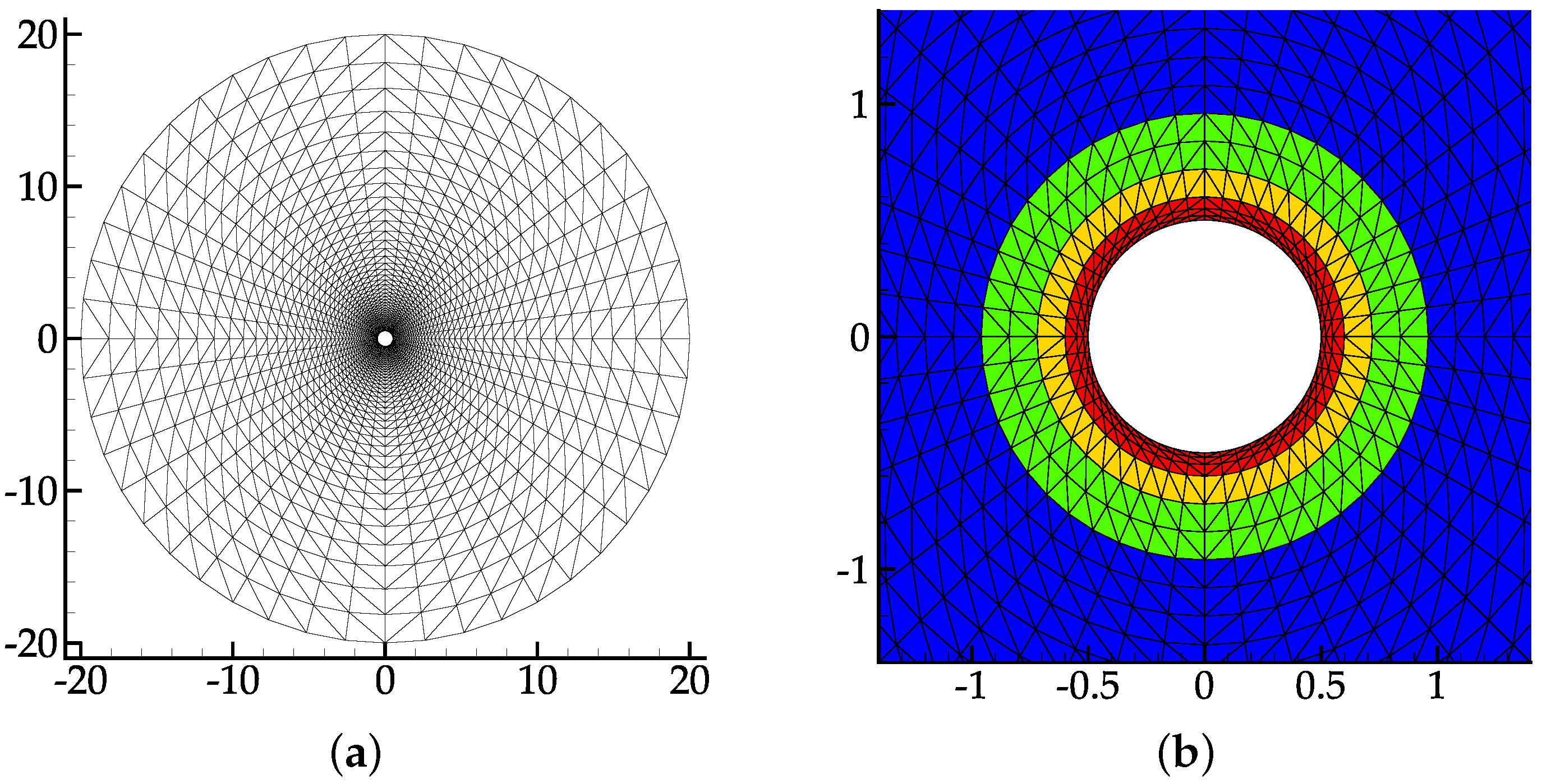
Figure 5a shows the mesh for the numerical simulation. It is generated in a way similar to that in Figure 14, [9] and Figure 10, [32]. The diameter for the outer boundary is 40 times as big as that for the cylinder. There are 3840 triangular elements in the mesh. They are achieved by diagonalizing 48 × 40 structured rectangular elements. The heights of the first five layers of elements adhering to the cylinder are 0.02, 0.03, 0.05, 0.12 and 0.12. In the first layer of elements, we achieve the maximum of the aspect ratio, 3.25, and the maximum of the skewness (measured by the normalized equiangular method), 0.72. The biggest size changes appear at the third and the fourth layers of elements, i.e., 0 . 12 / 0 . 05 = 2 . 4 . Within the mesh, the maximum and minimum of h k are 0.0607 and 0.0168, respectively, resulting in S 4 . Figure 5b presents the coloring of the elements. The coloring strategy is the same as in Table 8.
In our computation, the state for the free-stream is defined by:
b = ρ u v p = γ 0 . 3 0 1 ,
leading to Ma = 0 . 3 , with the Mach number calculated by Ma = u 2 + v 2 / c . Besides, the Reynolds number of the free-stream is set to Re = 150 . To speed up the simulation, our computation consists of two periods. In the first period, we pursue the steady inviscid solution to the problem. That is, the flow is governed by the 2D Euler system, with b defining the initial condition. During the computation, characteristic boundary conditions [33] and inviscid wall conditions are applied to the outer boundary and the cylinder surface, respectively. In the second period, the governing system for the problem is replaced by Equation (54). The inviscid solution just obtained is used for initializing the flow. Characteristic boundary conditions and viscous wall conditions [8] (p. 484) are applied during the remaining computation.
In our computation, N = 3 is taken for local approximations. The spatial discretization for the convective items are the same as that in Section 4.4. The NIPG approach for treating the viscous items can be found in [8] (pp. 486–491). To find the upper limit of C e m , we first integrate the DG discretization using the SSP-RK3 scheme, with the time step length defined by:
Δ t = 1 2 C e x ( 2 N + 1 ) · min Ω k T h h k λ k ,
where:
λ k = max x Ω k v · n k , v · n k c , v · n k + c + N Re r e f ρ h k .
where v = ( u , v ) , c = γ p / ρ , and h k is the dimensionless element size.
Through numerical tests, we found that the maximum of C e x for maintaining the calculation stability is 0.8. Next, the hybrid scheme with Δ t = 0 . 0025 is used for the time integration. The fixed time step length is close to one obtained by Equation (32) with d = 2 , C e m = 0 . 8 and C i m = 4 .
According to the direct numerical simulations (DNS) results in [34] and the experimental results referred to therein, the flow is unsteady with Ma = 0 . 3 and Re = 150 . Over time, vortices periodically shed from the cylinder, causing fluctuations in the physical quantities in the wake of the cylinder. 
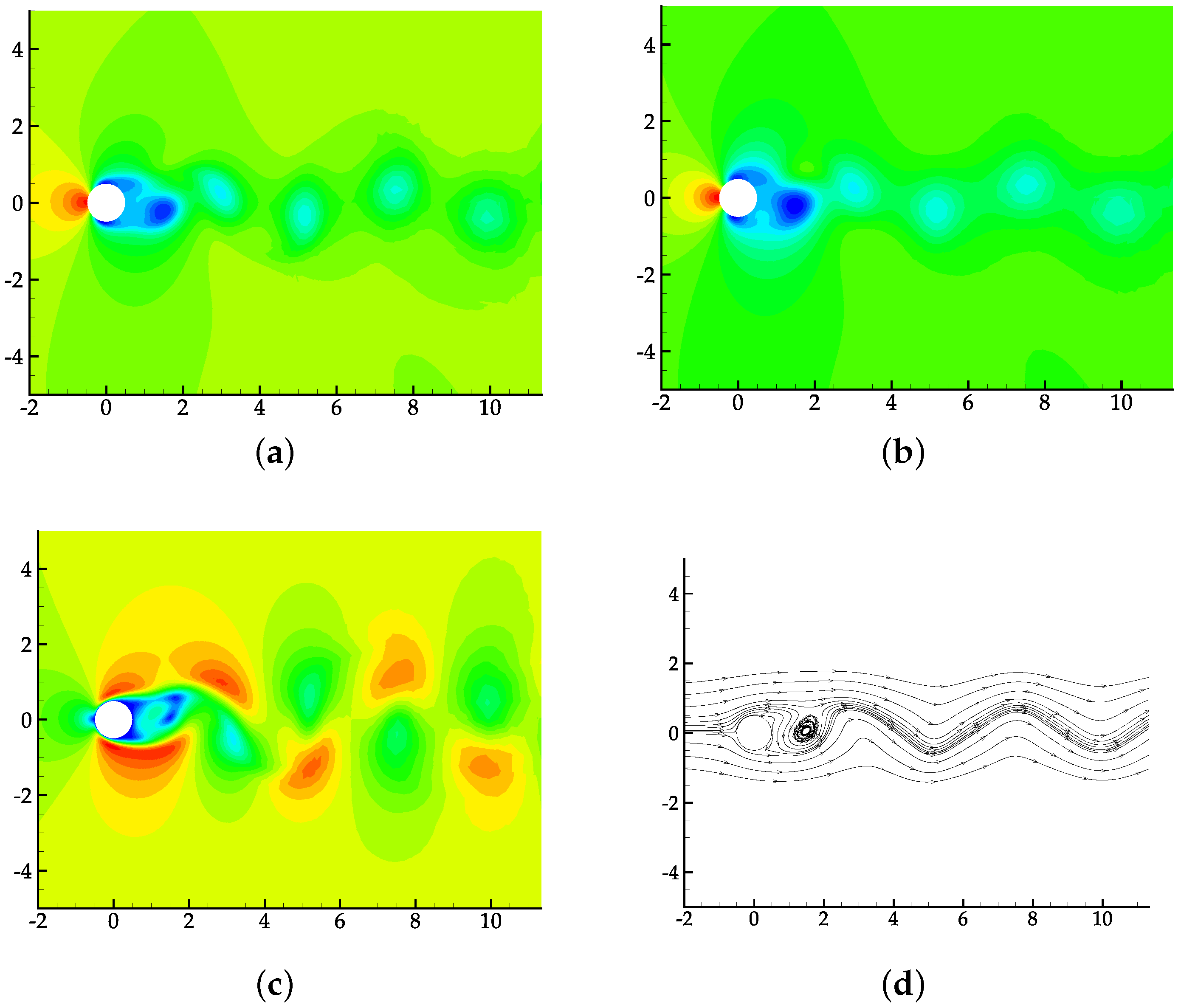
Figure 6 shows the numerical results at t = 408 
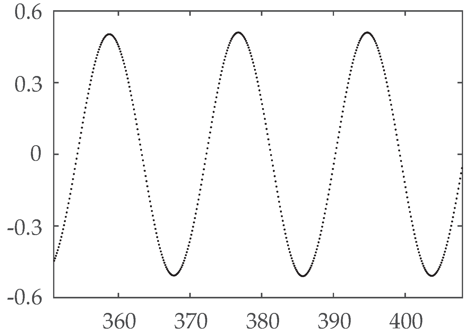
. The fluctuations in the fields and the bending of the streamlines indicate that the shedding of vortices has been set up well. During the calculation, the lift coefficient C L of the cylinder is recorded every 50 time steps. The time history for C L from t = 350 to t = 408 is shown in Figure 7. It can be found that the fluctuation period of C L is T s h e d = 18 . Table 10 compares our numerical results with that in reference [34]. The matches between the two sets of results illustrate the usefulness of the hybrid scheme.
Table 11 presents the available dimensionless time step length and the CPU time (in seconds) cost per time step for each scheme. After dividing the CPU time with the time step length for each scheme, we got the required CPU time for the simulation corresponding to unit dimensionless time, i.e., 2985 s for the SSP-RK3 scheme, 1923 s for the SSP-RK3-4 scheme and 1480s for our hybrid scheme. It is clear that the hybrid scheme performs best in terms of efficiency.

5. Conclusions

In this work, we developed a hybrid scheme for the temporal integration of the DG discretization for the unsteady convection-dominated problem. The hybrid scheme consists of two popular high-order schemes: the SSP-RK3 scheme and the LDIRK3 scheme. By separately treating the coarse elements and the refined elements with an explicit scheme and an implicit scheme, a time step bigger than that for a purely explicit scheme can be reached at a comparatively low cost. Using the independence of the local approximation for the DG method, we proposed a strategy of grouping the elements that is necessary for maintaining the stability and reducing the computing cost of the hybrid scheme. We tested our scheme by numerically solving several threshold problems. The matches between the numerical solutions and the reference results proved the usefulness of the hybrid scheme. The comparison with the traditional explicit schemes testified the effectiveness of the hybrid scheme on the meshes with certain level of geometry-induced stiffness.

Author Contributions

Conceptualization, methodology, software, validation, formal analysis, investigation, data curation, writing—original draft preparation, writing—review and editing, visualization: L.L.; resources, supervision, funding acquisition: S.W. All authors have read and agreed to the published version of the manuscript.

Funding

This research was funded by the National Natural Science Foundation of China, grant number 91530325.

Acknowledgments

The first author is sincerely thankful to Fujun Liu from the School of Mathematics and System Science, Beihang University for the advice on the setting for the last numerical test. The valuable suggestions given by the anonymous reviewers are deeply appreciated by the authors.

Conflicts of Interest

The authors declare no conflict of interest.

Appendix A

A new class of SSP-RK schemes was developed in reference [29]. By allowing the stage numbers bigger than the order numbers, the available CFL numbers for the new SSP-RK schemes are larger than those for the traditional SSP-RK schemes. A four-stage, third-order accurate scheme of this class is denoted by SSP-RK3-4. Its Butcher tableau is given as:
Energies 13 01870 i003
Similar to that in Section 3.4, we deduce the increment function for the scheme, i.e.,
R ( z ) SSP RK 3 4 = 1 + z + 1 2 z 2 + 1 6 z 3 + 1 48 z 4 ,
and plot the stability region in Figure A1. For more information of the SSP-RK3-4 scheme, the reader is referred to reference [29].
Figure A1. Absolute stability region for the SSP-RK3-4 scheme, interior of the blue line.
Energies 13 01870 g0a1

References

  1. Reed, W.; Hill, T. Triangular Mesh Methods for the Neutron Transport Equation; Technical Report LA-UR-73-479; Los Alamos Scientific Laboratory: Los Alamos, NM, USA, 1973. [Google Scholar]
  2. Cockburn, B.; Shu, C.-W. The Runge-Kutta local projection P1-discontinuous Galerkin finite element method for scalar conservation laws. Math. Model. Numer. Anal. 1991, 25, 337–361. [Google Scholar] [CrossRef]
  3. Cockburn, B.; Shu, C.-W. TVB Runge-Kutta local projection discontinuous Galerkin finite element method for conservation laws. II: General framework. Math. Comput. 1989, 52, 411–435. [Google Scholar] [CrossRef]
  4. Cockburn, B.; Lin, S.; Shu, C.-W. TVB Runge-Kutta local projection discontinuous Galerkin finite element method for conservation laws. III: One-dimensional systems. J. Comput. Phys. 1989, 84, 90–113. [Google Scholar] [CrossRef] [Green Version]
  5. Cockburn, B.; Hou, S.; Shu, C.-W. The Runge-Kutta local projection discontinuous Galerkin finite element method for conservation laws. IV: The multidimensional case. Math. Comput. 1990, 54, 545–581. [Google Scholar] [CrossRef]
  6. Cockburn, B.; Shu, C.-W. The Runge-Kutta discontinuous Galerkin method for conservation laws V: Multidimensional systems. J. Comput. Phys. 1998, 141, 199–224. [Google Scholar] [CrossRef]
  7. Hesthaven, J.S.; Warburton, T. Nodal Discontinuous Galerkin Methods: Algorithms, Analysis, and Applications, 1st ed.; Springer: New York, NY, USA, 2008. [Google Scholar]
  8. Dolejší, V.; Feistauer, M. Discontinuous Galerkin Method: Analysis and Applications to Compressible Flow, 1st ed.; Springer: Cham, Switzerland, 2015. [Google Scholar]
  9. Kanevsky, A.; Carpenter, M.H.; Gottlieb, D.; Hesthaven, J.S. Application of implicit-explicit high order Runge-Kutta methods to discontinuous-Galerkin schemes. J. Comput. Phys. 2007, 225, 1753–1781. [Google Scholar] [CrossRef] [Green Version]
  10. Kennedy, C.A.; Carpenter, M.H. Additive Runge–Kutta schemes for convection–diffusion–reaction equations. Appl. Numer. Math. 2003, 44, 139–181. [Google Scholar] [CrossRef]
  11. Dolean, V.; Fahs, H.; Fezoui, L.; Lanteri, S. Locally implicit discontinuous Galerkin method for time domain electromagnetics. J. Comput. Phys. 2010, 229, 512–526. [Google Scholar] [CrossRef] [Green Version]
  12. Hochbruck, M.; Sturm, A. Error analysis of a second-order locally implicit method for linear Maxwell equations. SIAM J. Numer. Anal. 2016, 54, 3167–3191. [Google Scholar] [CrossRef] [Green Version]
  13. Descombes, S.; Lanteri, S.; Moya, L. Temporal convergence analysis of a locally implicit discontinuous Galerkin time domain method for electromagnetic wave propagation in dispersive media. J. Comput. Appl. Math. 2017, 316, 122–132. [Google Scholar] [CrossRef] [Green Version]
  14. Gottlieb, S.; Shu, C.-W.; Tadmor, E. Strong stability-preserving high-order time discretization methods. SIAM Rev. 2001, 43, 89–112. [Google Scholar] [CrossRef]
  15. Gottlieb, S.; Shu, C.-W. Total variation diminishing Runge-Kutta schemes. Math. Comput. 1998, 67, 73–85. [Google Scholar] [CrossRef] [Green Version]
  16. Alexander, R. Diagonally implicit Runge-Kutta methods for stiff O.D.E.’s. SIAM J. Numer. Anal. 1977, 14, 1006–1021. [Google Scholar] [CrossRef]
  17. Cameron, I.T. Solution of differential-algebraic systems using diagonally implicit Runge-Kutta methods. IMA J. Numer. Anal. 1983, 3, 273–289. [Google Scholar] [CrossRef]
  18. Skvortsov, L.M. Diagonally implicit Runge–Kutta methods for stiff problems. Comput. Math. Math. Phys. 2006, 46, 2110–2123. [Google Scholar] [CrossRef]
  19. Li, L.; Wu, S. Construction of Jacobian matrix for solving convection-diffusion problem with interior penalty method. In Proceedings of the 2018 International Conference on Computer Information Science and Application Technology, Daqing, China, 7–9 December 2018. [Google Scholar] [CrossRef]
  20. Qiu, J.; Khoo, C.K.; Shu., C.-W. A numerical study for the performance of the Runge-Kutta discontinuous Galerkin method based on different numerical fluxes. J. Comput. Phys. 2006, 212, 540–565. [Google Scholar] [CrossRef]
  21. Bassi, F.; Rebay, S. A high-order accurate discontinuous finite element method for the numerical solution of the compressible Navier-Stokes equations. J. Comput. Phys. 1997, 131, 267–279. [Google Scholar] [CrossRef]
  22. Cockburn, B.; Shu, C.-W. The local discontinuous Galerkin method for time-dependent convection-diffusion systems. SIAM J. Numer. Anal. 1998, 35, 2440–2463. [Google Scholar] [CrossRef]
  23. Peraire, J.; Persson, P.-O. The compact discontinuous Galerkin (CDG) method for elliptic problems. SIAM J. Sci. Comput. 2008, 30, 1806–1824. [Google Scholar] [CrossRef] [Green Version]
  24. Cheng, J.; Yang, X.; Liu, X.; Liu, T.; Luo, H. A direct discontinuous Galerkin method for the compressible Navier-Stokes equations on arbitrary grids. J. Comput. Phys. 2016, 327, 484–502. [Google Scholar] [CrossRef]
  25. Persson, P.-O. Shock capturing for high-order discontinuous Galerkin simulation of transient flow problems. In Proceedings of the 21th AIAA Computational Fluid Dynamics Conference, San Diego, CA, USA, 24–27 June 2013. [Google Scholar] [CrossRef] [Green Version]
  26. Dumbser, M.; Zanotti, O.; Loubère, R.; Diot, S. A posteriori subcell limiting of the discontinuous Galerkin finite element method for hyperbolic conservation laws. J. Comput. Phys. 2014, 278, 47–75. [Google Scholar] [CrossRef] [Green Version]
  27. Segawa, H.; Luo, H.; Nourgaliev, R. A diagonally implicit Runge-Kutta method for the discontinuous Galerkin solutions of the Navier-Stokes equation. In Proceedings of the 49th AIAA Aerospace Sciences Meeting including the New Horizons Forum and Aerospace Exposition, Orlando, FL, USA, 4–7 January 2011. [Google Scholar] [CrossRef]
  28. Persson, P.-O.; Peraire, J. Newton-GMRES preconditioning for discontinuous Galerkin discretizations of the Navier-Stokes equations. SIAM J. Sci. Comput. 2008, 30, 2709–2733. [Google Scholar] [CrossRef]
  29. Spiteri, R.J.; Ruuth, S.J. A new class of optimal high-order strong-stability-preserving time discretization methods. SIAM J. Numer. Anal. 2002, 40, 469–491. [Google Scholar] [CrossRef]
  30. Zhang, F.; Cheng, J.; Liu, T. A direct discontinuous Galerkin method for the incompressible Navier-Stokes equations on arbitrary grids. J. Comput. Phys. 2019, 380, 269–294. [Google Scholar] [CrossRef]
  31. Dolejší, V.; Feistauer, M. A semi-implicit discontinuous Galerkin finite element method for the numerical solution of inviscid compressible flow. J. Comput. Phys. 2004, 198, 727–746. [Google Scholar] [CrossRef]
  32. Barter, G.E.; Darmofal, D.L. Shock capturing with PDE-based artificial viscosity for DGFEM: Part I. Formulation. J. Comput. Phys. 2010, 229, 1810–1827. [Google Scholar] [CrossRef]
  33. Abarbanel, S.S.; Don, W.-S.; Gottlieb, D.; Rudy, D.H.; Townsend, J.C. Secondary frequencies in the wake of a circular cylinder with vortex shedding. J. Fluid Mech. 1991, 225, 557–574. [Google Scholar] [CrossRef] [Green Version]
  34. Inoue, O.; Hatakeyama, N. Sound generation by a two-dimensional circular cylinder in a uniform flow. J. Fluid Mech. 2002, 471, 285–314. [Google Scholar] [CrossRef]
Figure 1. Elements grouping for a one-dimensional (1D) mesh.
Energies 13 01870 g001
Figure 2. Absolute stability regions for different schemes. (a) SSP-RK3, interior of the black line. (b) LDIRK3, exterior of the red line.
Energies 13 01870 g002
Figure 3. Coarse 1D mesh.
Energies 13 01870 g003
Figure 4. (a) Coarse 2D mesh for the isentropic vortex problem. (b) Elements coloring for Coarse 2D. (c) Zoom in for T h , i m of Coarse 2D.
Energies 13 01870 g004
Figure 5. (a) Mesh for the flow around cylinder. (b) Elements coloring for the mesh.
Energies 13 01870 g005
Figure 6. Numerical results for the flow over a cylinder, t = 408 . (a) Contours for ρ ρ , 20 equally spaced from −0.13 to 0.06. (b) Contours for p p , 20 equally spaced from −0.09 to 0.07. (c) Contours for Ma, 20 equally spaced from 0 to 0.43. (d) Stream lines plot.
Energies 13 01870 g006
Figure 7. Time history of C L , t =350–408, flow around a cylinder.
Energies 13 01870 g007
Table 1. L 2 errors, 1D linear advection problem.
Mesh L 2 ErrorOrder
Coarse 1D 1 . 76 × 10 3
Middle 1D 2 . 35 × 10 4 2.90
Fine 1D 2 . 97 × 10 5 2.98
Table 2. Comparison of different schemes, 1D linear advection problem.
Mesh Δ t RK 3 Δ t RK 3 4 Δ t hybrid T CPU , RK 3 / s T CPU , RK 3 4 / s T CPU , hybrid / s
Coarse 1D 4 . 0 × 10 3 8 . 0 × 10 3 4 . 0 × 10 2 3.732.141.46
Middle 1D 2 . 0 × 10 3 4 . 0 × 10 3 2 . 0 × 10 2 7.463.902.84
Fine 1D 1 . 0 × 10 3 2 . 0 × 10 3 1 . 0 × 10 2 14.517.474.59
Table 3. L 2 errors, 1D linear advection-diffusion problem.
Mesh L 2 ErrorOrder
Coarse 1D 6 . 56 × 10 3
Middle 1D 1 . 45 × 10 3 2.18
Fine 1D 3 . 10 × 10 4 2.23
Table 4. Comparison of different schemes, 1D linear advection-diffusion problem.
Mesh Δ t RK 3 Δ t RK 3 4 Δ t hybrid T CPU , RK 3 / s T CPU , RK 3 4 / s T CPU , hybrid / s
Coarse 1D 6 . 7 × 10 4 1 . 3 × 10 3 6 . 7 × 10 3 2.351.400.97
Middle 1D 2 . 5 × 10 4 5 . 0 × 10 4 2 . 5 × 10 3 5.813.352.53
Fine 1D 8 . 3 × 10 5 1 . 7 × 10 4 8 . 3 × 10 4 17.5510.845.98
Table 5. L 2 errors, density, 1D Euler system.
Mesh L 2 ErrorOrder
Coarse 1D 4 . 62 × 10 5
Middle 1D 5 . 89 × 10 6 2.97
Fine 1D 7 . 52 × 10 7 2.97
Table 6. Comparison of different schemes, 1D Euler system.
Mesh Δ t RK 3 Δ t RK 3 4 Δ t hybrid T CPU , RK 3 / s T CPU , RK 3 4 / s T CPU , hybrid / s
Coarse 1D 6 . 9 × 10 4 1 . 4 × 10 3 6 . 9 × 10 3 13.257.467.00
Middle 1D 3 . 4 × 10 4 6 . 9 × 10 4 3 . 4 × 10 3 24.6013.6611.51
Fine 1D 1 . 7 × 10 4 3 . 4 × 10 4 1 . 7 × 10 3 45.2427.7122.51
Table 7. Coloring strategy for 2D meshes.
GroupColor
T h , i m red + yellow
T h , e x green + blue
T h , e x 1 yellow + green +blue
T h , e x 2 yellow + green
Table 8. L 2 errors, density, 2D Euler system.
Mesh L 2 ErrorOrder
Coarse 2D 1 . 32 × 10 3
Middle 2D 1 . 84 × 10 4 2.84
Fine 2D 2 . 44 × 10 5 2.91
Table 9. Comparison of different schemes, 2D Euler system.
Mesh Δ t RK 3 Δ t RK 3 4 Δ t hybrid T CPU , RK 3 / s T CPU , RK 3 4 / s T CPU , hybrid / s
Coarse 2D 1 . 1 × 10 3 2 . 3 × 10 3 1 . 2 × 10 3 1047838
Middle 2D 5 . 8 × 10 4 1 . 2 × 10 3 6 . 2 × 10 3 832568262
Fine 2D 2 . 9 × 10 4 5 . 8 × 10 4 3 . 1 × 10 3 781562542349
Table 10. Results comparison, 2D Navier-Stokes system.
DataStrouhal Number C L Amplitude
Numerical0.1850.51
Reference0.1830.52
Table 11. Comparison of different schemes, 2D Navier-Stokes system.
Δ t RK 3 Δ t RK 3 4 Δ t hybrid Δ T CPU , RK 3 / s Δ T CPU , RK 3 4 / s Δ T CPU , hybrid / s
6 . 7 × 10 4 1 . 3 × 10 3 2 . 5 × 10 3 2.02.53.7

