Abstract
A dynamic Smagorinsky–Lilly model (DSLM) subgrid model on the basis of the Smagorinsky–Lilly subgrid model (SLM) was introduced in the OpenFOAM software. The flow field of the vehicle was simulated, and the pressure coefficient and sound pressure curve of the monitoring points were compared with the wind tunnel test results. The results show that the DSLM subgrid model with a wall function can achieve high simulation accuracy. The investigation of the flow field structure revealed an intermittent detachment of the turbulent vortex after the airflow passed through the rearview mirror, thereby resulting in a violent pressure pulsation on the side window around the rearview mirror. Airflow passed through the A-pillar, separated, and reattached on the upper side window, thereby producing aerodynamic noise. The research results can serve as a good reference for the simulation and test of aerodynamic noises outside the vehicle, and for the reduction of the aerodynamic noises of vehicles.
1. Introduction
Passenger comfort has become increasingly important along with improvements in automobile performance and increasing consumer demands. Noise is a form of energy. At high speed, the airflow out of vehicles can produce aerodynamic noise, thereby substantially affecting passenger comfort [1,2]. The aerodynamic noise produced by vehicles during driving can be mainly divided into leak, cavity, wind whistling, and wind turbulence noises.
When vehicles suffer from poor sealing, the pressure difference between the vehicle surface and interior can allow air flow through the leak gap, thereby causing leak noise. Cavity noise is the response of the cab cavity to the unsteady air flow at the opening when the side window or sunroof is opened. Such a response shows the periodic change in pressure inside the cavity. Wind whistling noise is from the periodic vortex shedding caused by rod-shaped objects exposed to high-speed airflow, such as vehicle antennas and luggage racks. The majority of the wind turbulence noises originate from the intense pressure pulse on the side window surface caused by the A-pillar vortex and complex wake structures behind the exterior rearview mirror in the side window area [3,4].
At present, two methods can be used to study aerodynamic noises: experimental and numerical simulations. Experimental simulation measures the pressure fluctuation or noise value of a target area through road and wind tunnel tests or by capturing the structure of the flow field and analyzing the relationship between flow and aerodynamic noise [5,6].
Donald P. Iacovoni et al. of Ford Motor Company [7] conducted experiments to optimize the use of cars’ rearview mirrors in reducing aerodynamic noise. Experiments in the Lockheed low-speed wind tunnel identified the key dimensions of the noise-reducing rearview mirror: the section shape of the base and angle between the base and the side window.
General Motors’ Bahram khalighi and NASA’s Richard G. Lee et al. [8] analyzed the wake field of the rearview mirror through the particle image velocity technology and studied the influence of the wake structure on the aerodynamic noise.
Yang Bo from Jilin University [9] performed wind tunnel tests on Audi C5. Oil film flow display was used on the rearview mirror, A-pillar, and side window area; and the pressure fluctuation on the key components of the vehicle body to analyze the mechanism of the aerodynamic noise generation on these areas.
Li Wenwu and Liu Ningning et al. [10] performed a road test and transfer path analysis to investigate the transfer characteristics of aerodynamic noise outside a vehicle under high-speed condition. The aforementioned studies evaluated the aerodynamic noise on the driver’s ear side and analyzed the contribution characteristics of the different types of noise sources outside a vehicle with a change in vehicle speed.
Atsushi Itoh and ZongGuang Wang [11] conducted bench and road tests to study the noise produced by the refrigerant flow of automobile air conditioner. A high-speed camera was used to capture the flow process, and the correlation of the flow, velocity, and noise was analyzed using the image.
Yang Jianguo, Zhang Siwen, and others [12] measured the aerodynamic noise of a car in the automobile wind tunnel in Tongji University to improve and optimize the main components of a car’s body and reduce aerodynamic noise. The test results showed that the gap between the body surface and parts of the sealing system contributes to interior wind noises, which are distributed in a specific frequency band.
Although wind tunnel and road test technologies of aerodynamic noises are relatively mature, the latter is substantially influenced by the external environment (i.e., with high environmental requirements) and can only be performed after the production of sample vehicles. By contrast, wind tunnel test is minimally affected by the environment and can be used in the early stage of vehicle design. However, this type of test consumes enormous human, material, and financial resources. The development of computer technology has resulted in the increasing application of numerical simulations in the investigation of aerodynamic noises. In particular, numerical simulation can save cost and shorten the development cycle.
Kuo Huey Chen et al. of General Motors [13] performed a numerical simulation on the A-pillar water tank of a car. The subgrid model used was a large eddy simulation (LES) method of the Smagorinsky–Lilly model (SLM) for transient simulation. The sound propagation issue was addressed through an integration method. The simulation results were more accurate than the test results.
M. Islam and F. Decker of the Audi wind tunnel center [14] used the open source Computational Fluid Dynamics software OpenFOAM to simulate and analyze the external flow field of automobiles by using the detached eddy simulation (DES). The pressure coefficient of the body surface was consistent with the experimental value.
Sinisa Krajnovic [15] used LES to simulate and analyze the external flow field of vehicles. Compared with the results of the wind tunnel test, the simulated surface pressure and lateral force coefficients of the vehicle substantially approximated the test results. However, the grid near the wall is required in the LES method.
Li Qiliang and Du Wenhai [16] used LES and the sound disturbance equation to address the aerodynamic noise in the rearview mirror area. The difference in the simulation and test results was only 2.3 dB, and the spectrum trends of both methods were the same. Consequently, the active jet model was established to reduce the intensity of the eddy in the rearview mirror area to reduce the aerodynamic noise.
Jiang Hao et al. [17] proposed a fast optimization method of aerodynamic noise on the basis of the calculation of the flow field outside vehicles. In unsteady numerical simulations, the aerodynamic noise of the side window is analyzed by separating vortex simulation and computational aeroacoustics. The results showed that the intensity of the aerodynamic noise source in the optimized rear side window surface weakens in each frequency band, and the sound pressure level of each monitoring point is reduced.
However, improving the simulation accuracy (i.e., difference between the simulation and experimental results) is challenging. If simulation results are sufficiently accurate, then human and material resources can be conserved.
Automotive aerodynamic noises are produced by the vehicle exterior’s unsteady flow field; thus, the unsteady separation flow characteristics caused by the local details should be accurately obtained [18,19].
At present, the turbulent structure in the flow field can be solved using indirect and direct numerical simulations (DNS).
DNS is the most accurate method used to solve transient fluid control equation without introducing an additional turbulence model. However, the demand for computing resources is high and solving complex engineering problems using the current computing conditions is difficult. DNS is generally used in the mechanism research of simple models at low Reynolds number. The indirect numerical simulation methods do not directly calculate the pulsation characteristics of the turbulence, but approximate and simplify the turbulence. These methods include LES, DES, and Reynolds average Navier–Stokes.
LES, which possesses the combined advantages of DNS and mode theory, has been widely used in various numerical methods to study turbulent flows [20,21]. In recent years, many studies have used LES to investigate and analyze automotive aerodynamics. However, meeting the requirements of near-wall areas entails the division of numerous meshes, thereby introducing difficulties in the calculation. The subgrid model is an important component of LES. A considerably rough mesh near the wall signifies the substantial dependence of the simulation precision on the subgrid model. Piscaglia et al. [22] used the OpenFOAM platform to improve the wall processing method and subgrid model, and utilized the model thereafter to simulate flow fields with complex geometries. Serre et al. [23] simulated the turbulent flows of the Ahmed model tail to evaluate the applicability of LES. Kundan Biswas et al. [24] used LES to predict vehicles’ drag coefficient by utilizing the OpenFOAM tool.
Although the calculation results of LES with wall function and subgrid model approximate those obtained using the wind tunnel test, the influence of the aerodynamic noise on the simulation precision is not considered. Along with the development in the field of aeroacoustics, progress has been evident in the investigation of the A-pillar and rearview mirror areas. The current study aims to explore the applicability of LES in predicting the exterior vehicle aerodynamic noise and its influence on the simulation precision.
This study uses the OpenFOAM platform in applying LES with wall function to simulate the automobile external flow field, and obtain and compare the pressure coefficient and curve of the sound pressure level with those determined using the wind tunnel test. This research also summarizes the influence of LES with different subgrid models on the precision of car exterior aerodynamic noise simulations, and explores the noise generation mechanism on the side window around the rearview mirror.
2. Computational Theory
2.1. LES
The general forms of the equations of the transient state used in the LES method are as follows [25]:
and
where the parameters with an overline represent the filtered field variables, and denote the velocity components after filtering, represents the fluid density, and denotes the dynamic viscosity. The sub-grid stress can be expressed as follows:
Following the Boussinesq approximation, the sub-grid stress can be calculated as follows:
where denotes the turbulent viscous force of the subgrid, is the isotropic part of the subgrid, represents the strain rate, and denotes the stress tensor rate, which is defined as follows:
2.2. SLM Subgrid Model
The SLM subgrid model is established on the basis of isotropy according to the mixing length model of Prandtl. This model describes the relationship between length and velocity as follows:
where is the mesh size alongside the axis, (i.e., Smagorinsky coefficient) denotes the empirical coefficient of SLM, and the mean flow stress results in different values of .
2.3. Dynamic SLM Ssubgrid Mmodel
When the SLM subgrid model is used to solve the , is constant, which is the main drawback of this model. Consequently, the simulation accuracy of the SLM model is poor. When the DSLM subgrid model is used, is no longer constant. Moreover, can be calculated using the 9th equation according to the solution of the moving vortex [26]. The DSLM method can describe the vortex structure more accurately than SLM.
where , which is the turbulent stress tensor that can be defined as follows:
is the subgrid turbulent stress obtained by twice filtering, and it can be expressed as follows:
and can be expressed as follows:
In these functions, the symbol “” means variables after mesh filtering and the symbol “”means variables after verified filtering.
The DLSM model was introduced by Germano et al. [27], who made an important contribution to the development of subgrid model because of making the calculation result more accurate. They obtained the turbulent stress tensor by adding two types of filter functions, namely, the mesh and test filter functions. The DSLM model considers the distance to the wall and obtains the dynamic solution of . Given that the average flow stress yields different values, the predictions of this model for the influence of a small vortex on a large eddy differ from those presented in previous research. Therefore, when LES is used to simulate the flow field, should be adjusted or a considerably accurate model should be adopted.
2.4. Acoustic Analogy Method Based on the Ffowcs Williams-Hawkings Equation
The acoustic analogy method based on the Ffowcs Williams–Hawkings (FW–H) equation utilizes CFD and acoustic software to simulate the aerodynamic noise.
After its introduction by Ffowcs Williams and Hawkings in 1969, the FW–H equation, which is also known as Lighthill’s acoustical analogy theory, was applied to moving solid boundary problems.
where is the sound velocity, is the sound pressure, is the time, is the far-field density, and are the velocities of the flow field and solid sound source surface, respectively, is the unit normal vector, is the axis direction, is the compressive stress tensor, and the subscripts i and j denote the i and j directions, respectively, in the selected sound field.
The acoustic analogy method is used to separately calculate the generation and propagation of sound. Compared with the direct calculation method, the calculation amount in the acoustic analogy method is substantially reduced. By solving the FW–H equation, the sound pressure level spectrum and total sound pressure level can be obtained. First, the flow field is transiently simulated using LES. Second, the results of LES is used to perform the Fourier transform. Lastly, the FW–H equation is solved, the sound field is simulated, and the acoustic results are obtained.
3. The Experimental Introduction
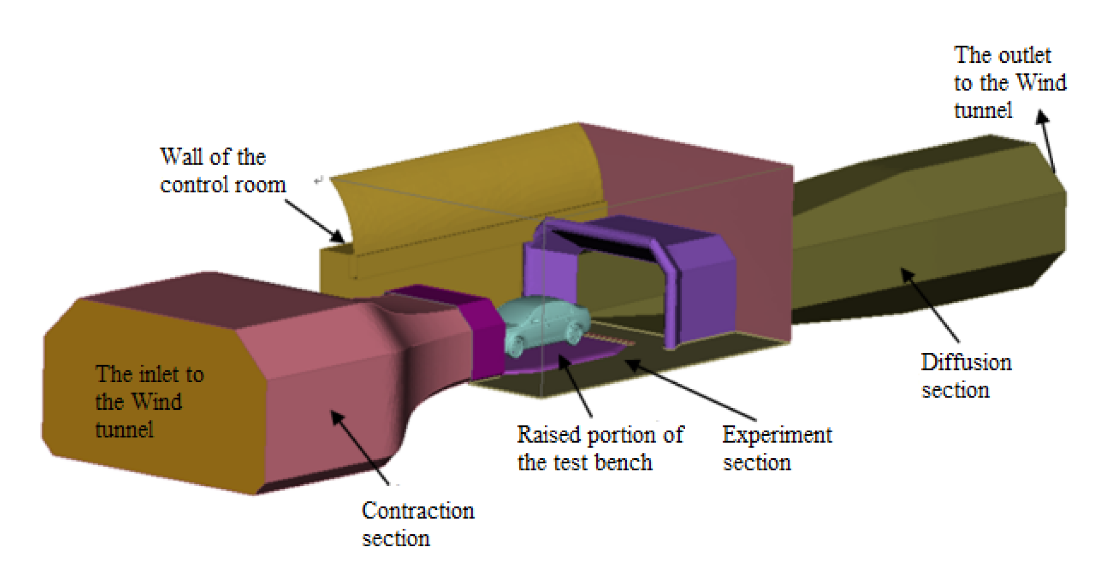
Wind tunnel experiments are performed in the Automotive Wind Tunnel Laboratory of Jilin University. It is a circumfluence wind tunnel with an open test section, which is 8 m × 4 m × 2.2 m. The shrinkage rate of the wind tunnel is 5.17 and the turbulence intensity . The structure of the wind tunnel is an open-jet type (Figure 1). When the frequency of the air flow pulsation in the test section coincides with the natural frequency of the test section, resonance will occur, which has a great impact on the safety and accuracy of the experiment. The natural frequency of the test section of the wind tunnel is about 20 Hz. When the velocity of the nozzle is 90 km/h, the resonance is more intense, so the speed of 90 km/h should be avoided. The research showed that when the wind speed in the test section exceeds 100 km/h, the external noise can be measured.
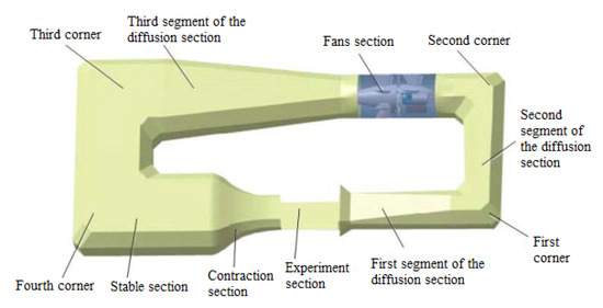
Figure 1.
Wind tunnel in Jilin University.
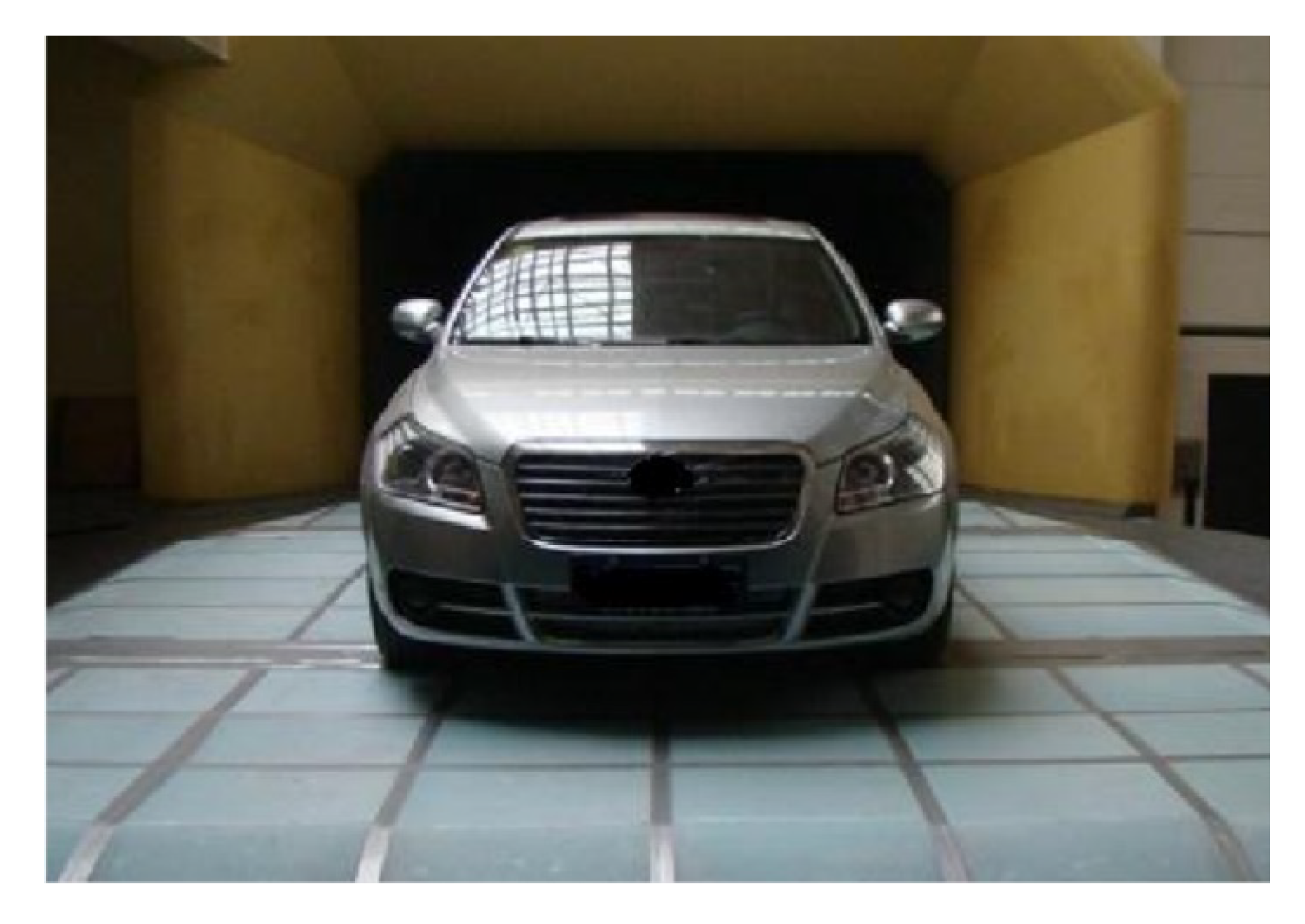
A real vehicle with wheels is fixed in the grooves on the test bench. In order to eliminate the noise caused by grooves, it is necessary to add foam board around the groove and fix it with adhesive tape. The front grille of the vehicle was closed in the test. The distance between vehicle front end and nozzle is 1m, the longitudinal symmetry of vehicle is overlapped with the center line of the test bench as shown in Figure 2. The test wind speed is 120 km/h.

Figure 2.
Test layout.
3.1. Surface Pressure Measuring
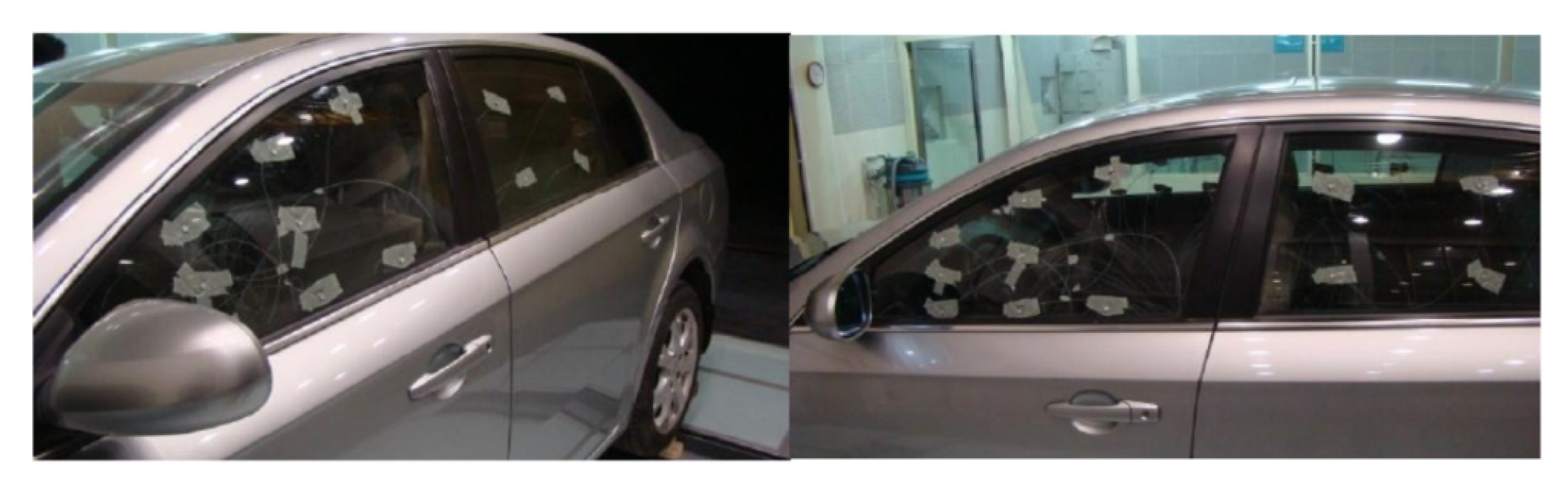
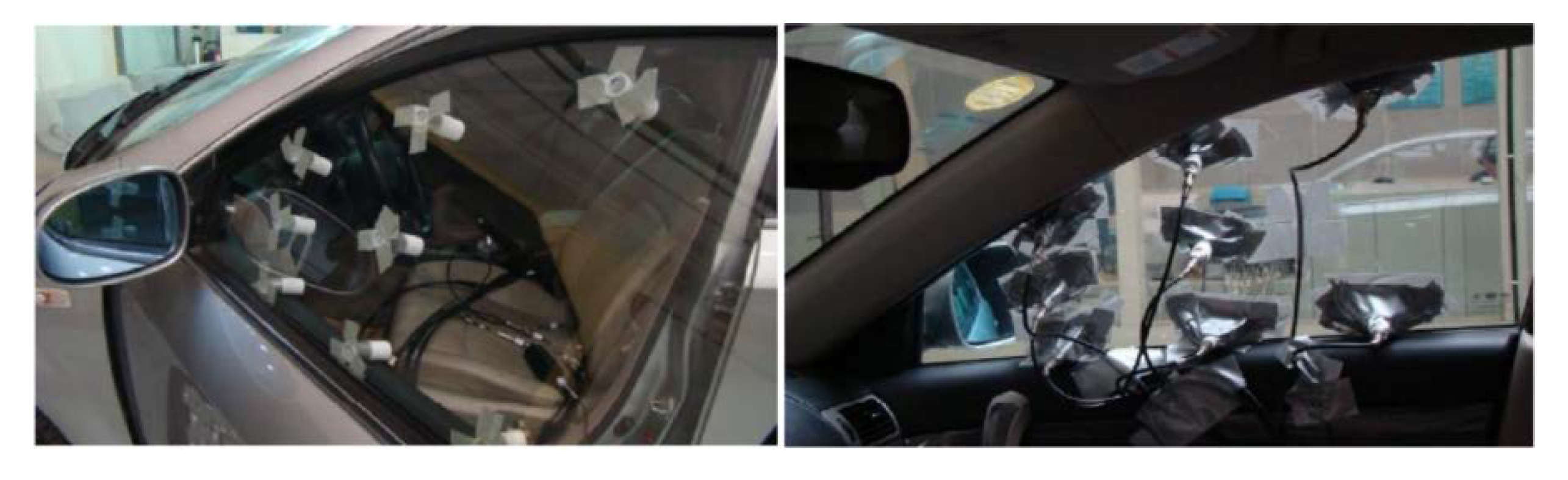
The flow field structure outside vehicles can be analyzed using the pressure distribution on the body surface. The wake structure of the rearview mirror significantly influences the pressure on the side window surface. Hence, the pressure pulsation information on the side window must be measured. Accordingly, holes should be drilled on the window to facilitate the arrangement of the pressure tube. Thereafter, the pressure-measuring tube is sealed and fixed using tape, and 12 monitoring points are arranged on the left and right sides (Figure 3).

Figure 3.
Layout to measure surface pressure.
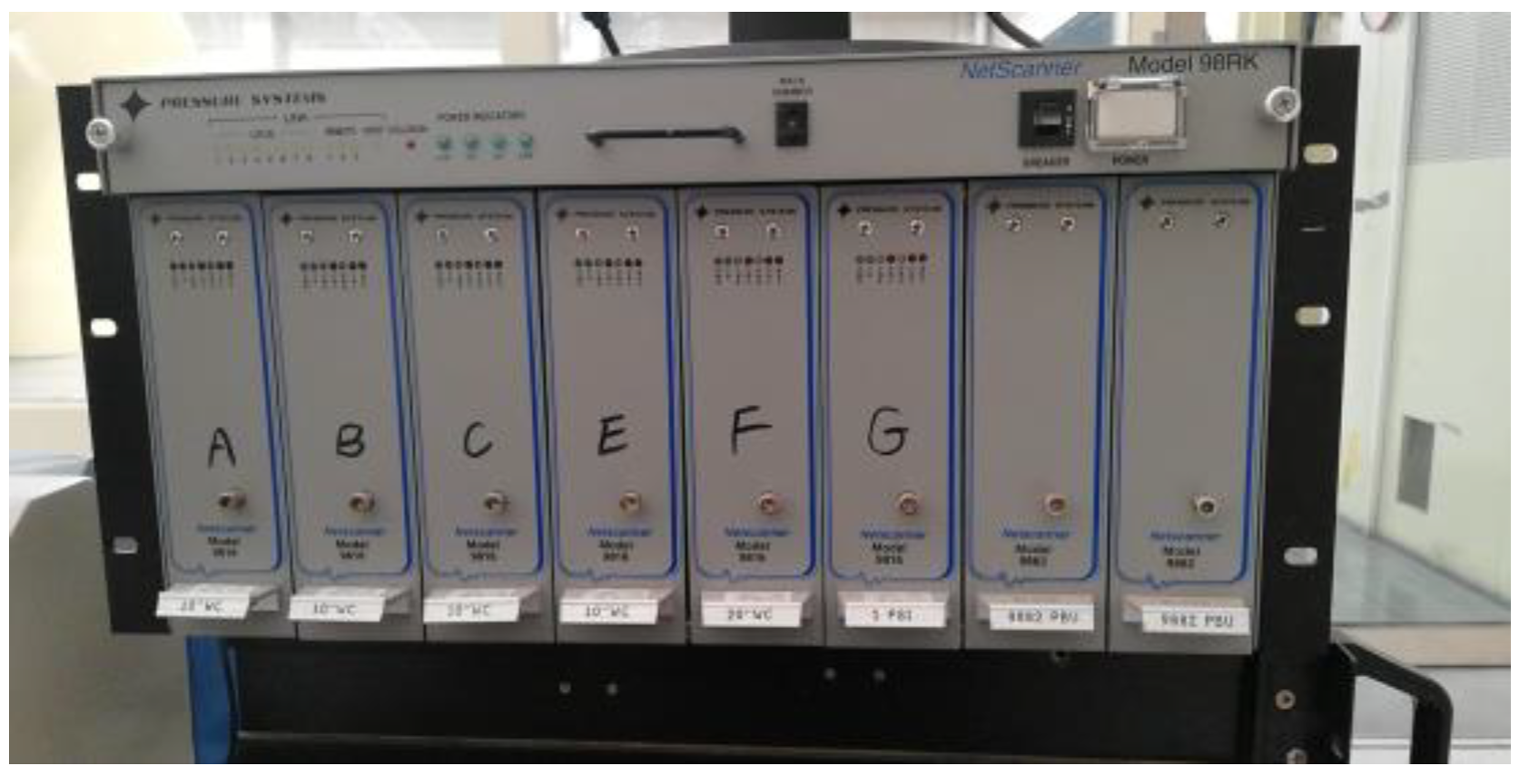
The other end of the tube is connected to a pulsating pressure collector, which is a pressure systems net scanner (model 98RK) (Figure 4). The sampling frequency is set to 50 Hz. Each pressure tube should be inspected for leaks and the collector should be set to 0 before the measurement.
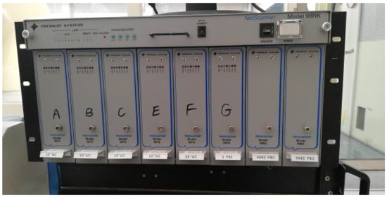
Figure 4.
Pressure-scanning instrument.
3.2. Surface Noise Intensity Measuring
Noise intensity should be determined after measuring the pressure on the side window area. The measuring position is consistent with the pressure-measuring position.
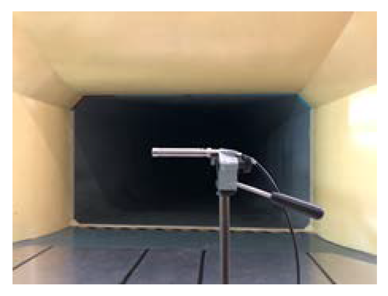
Given that a noise sensor is expensive and can be easily damaged, this equipment should be covered with a nylon sleeve for protection during the arrangement and fixed using tape to avoid shaking during the test. Moreover, the sensor should be maintained even with the glass to prevent unnecessary noise from affecting the accuracy. Before performing the actual vehicle test, background noise should be measured to determine whether it constitutes interference. Sensors are placed in the wind tunnel test section (Figure 5).

Figure 5.
Measuring site of the background noise.
After the sensor is calibrated, the wind tunnel is opened for gradual acceleration. When wind speed is 120 km/h and the air velocity of the test section is stable, the sensor starts to collect the noise signal. The total sound pressure level is 90.94 dB, and the highest value of the background noise appears in the low frequency band (0–1000 Hz) (Figure 6). The effect on the measured noise is negligible when the measured noise is higher than the background noise by over 10 dB.
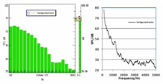
Figure 6.
Background noise level when v = 120 km/h.
After measuring the background noise, the noise intensity of side window was collected. The test layout is shown in Figure 7.

Figure 7.
Layout to measure noise intensity.
4. Numerical Simulation
4.1. Simulation Model
The model for the simulation is the same as that for the test. The model dimensions are shown in Figure 8. The length, width, height, and wheelbase of the vehicle are 4.688, 2.03, 1.44, and 2.65 m, respectively.
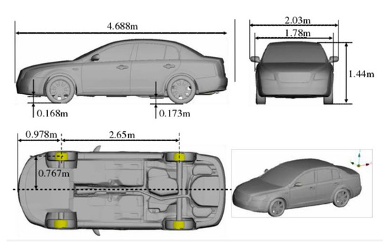
Figure 8.
Geometrical size of the vehicle model.
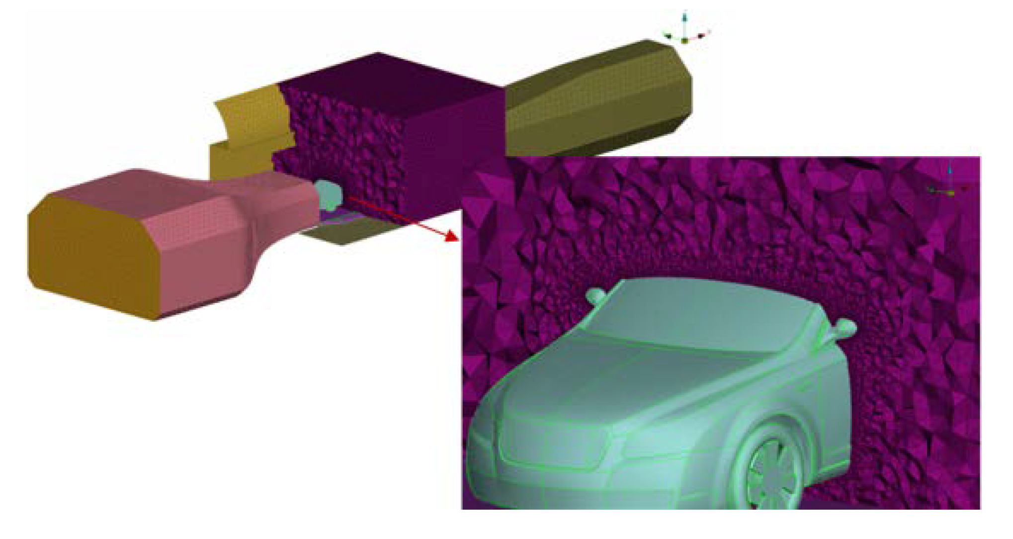
The computational domain is established on the basis of the wind tunnel structure (Figure 9). The computational domain mainly consists of the stable, contraction, test, and diffusion sections. The test section is 6.65 m long and 5.5 m high. The distance between the front end of the test car and nozzle is 1.0 m.
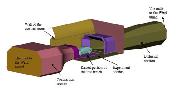
Figure 9.
Computational domain.
4.2. Mesh
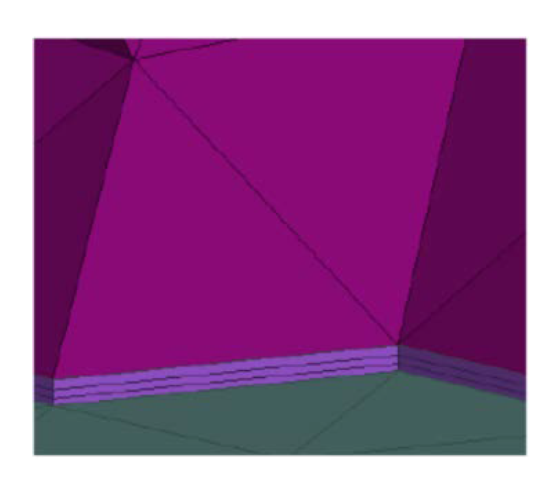
The unstructured grid used in the simulation involves triangular, triangular prism, and tetrahedron grids. The triangular grid is applied on the surface of the vehicle model, the simulation of the boundary layer flow is completed by stretching the triangular prism grid near the wall, and the tetrahedron grid is used in the other areas. The minimum grid size of the rearview mirror is 1.5 mm, whereas that of the key domain of the side window is 5 mm. The mesh of computational domain is from 20 mm to 400 mm. The mesh settings are shown in Table 1. The volume grids and boundary layer grids are shown in Figure 10 and Figure 11.

Table 1.
Mesh settings
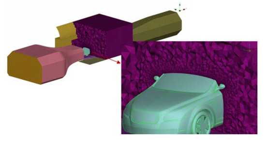
Figure 10.
Volume grids.

Figure 11.
Boundary layer grids.
To improve the calculation efficiency, two meshing forms are used according to the flow field mapping method in OpenFOAM. First, the steady flow field is obtained from the rough mesh. Secondly, the steady flow field result is projected into the dense mesh form using a mapping method to improve the calculation efficiency.
4.3. Boundary Condition
The inlet is set as the speed inlet (V = 6.44 m/s), and the velocity at the nozzle of the wind tunnel after the contraction section is 33.33 m/s (120 km/h). The outlet is set as the pressure outlet, and the specific boundary conditions are listed in Table 2.
Table 2.
Boundary condition settings.
The hydraulic diameter is four times the channel area divided by the perimeter of the channel section area. The hydraulic diameters of the inlet and outlet can be achieved using the wind tunnel mode.
4.4. Transient Solution Settings
The transient solution settings are summarized in Table 3.
Table 3.
Transient solution settings.
In the transient calculation, the time step is closely related to the convergence and accuracy of the simulation. Therefore, the appropriate time step should be selected. To ensure that the Courant number is below 1, the following formula is applied to set the time step:
where is the smallest grid scale and is the speed. The physical time step based on the grid scale is .
5. Simulation Results and Analysis
5.1. Simulation Results of Flow Field
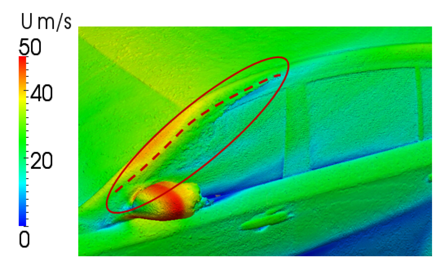
Through two subgrid models, the flow field structure near the side window is obtained, as shown in the Figure 12 and Figure 13. During the course of flowing through the A-pillar to the side window, the airflow separated and eddy region are formed (red circle in Figure 12). After the separation, some airflows in this area are attached to the side window and top beam (attachment line is denoted by the dotted line in Figure 12). Consequently, the flow field structure in this region is complex.
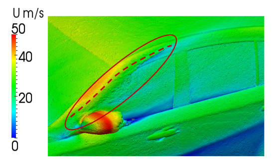
Figure 12.
Velocity distribution on the side window obtained using the SLM method at t = 0.765 s.
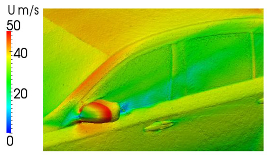
Figure 13.
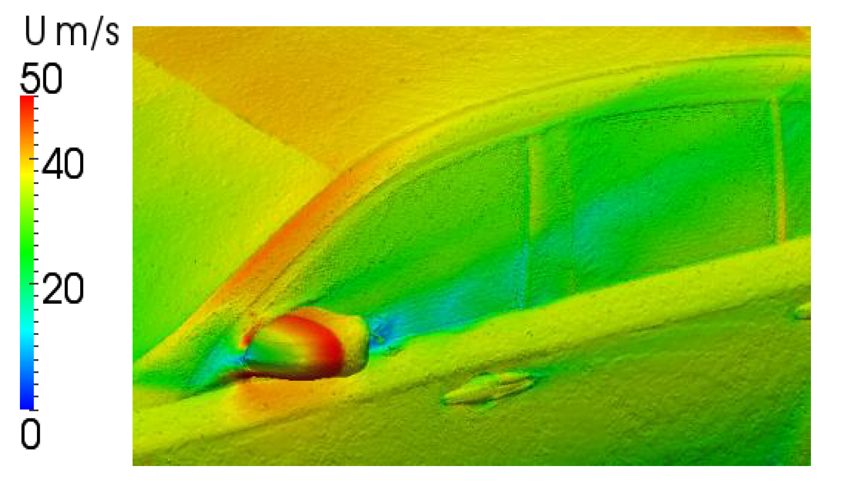
Velocity distribution on the side window obtained using the DSLM method at t = 0.765 s.
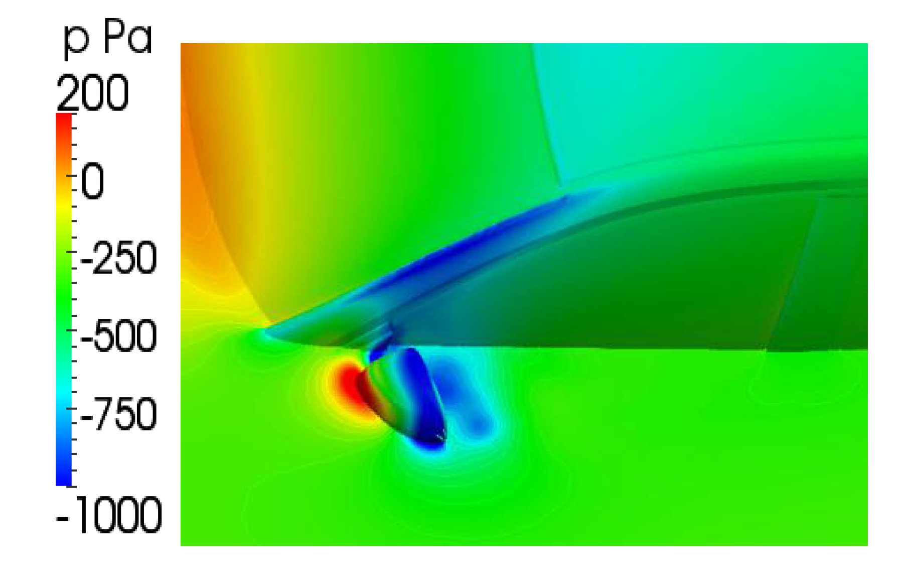
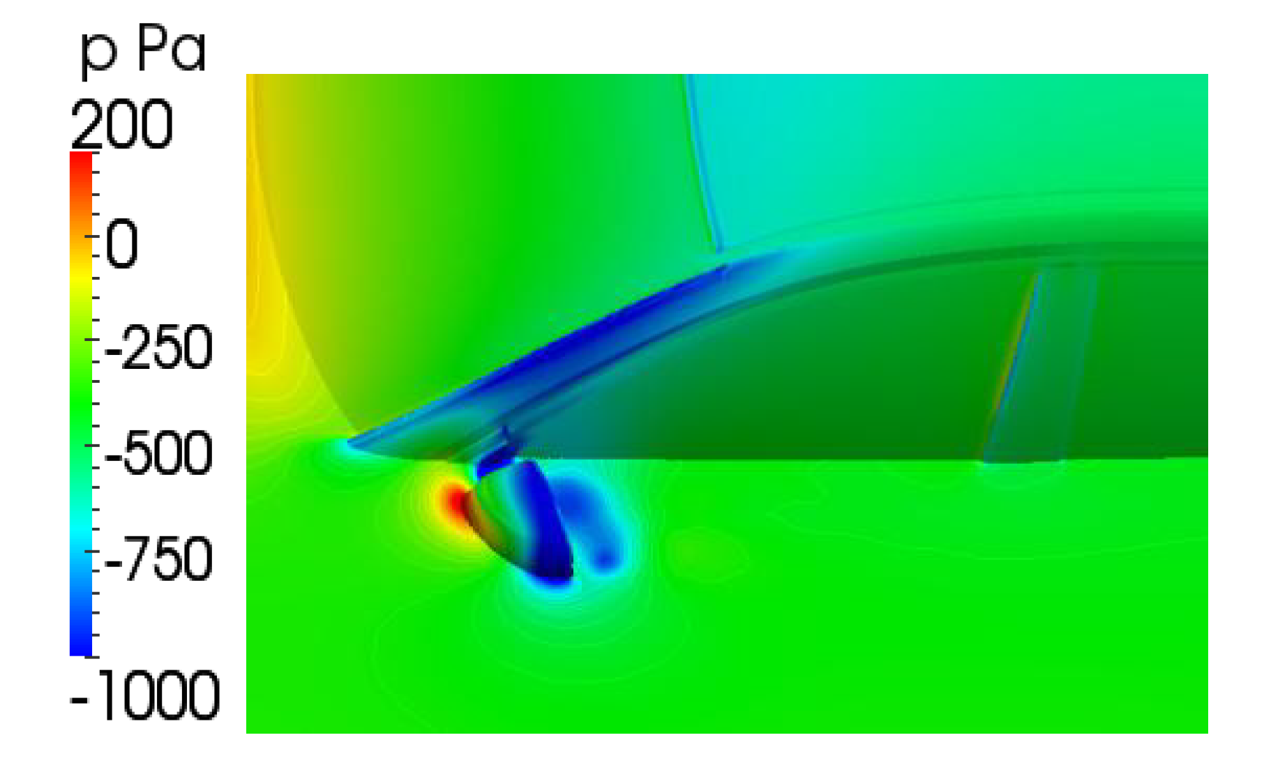
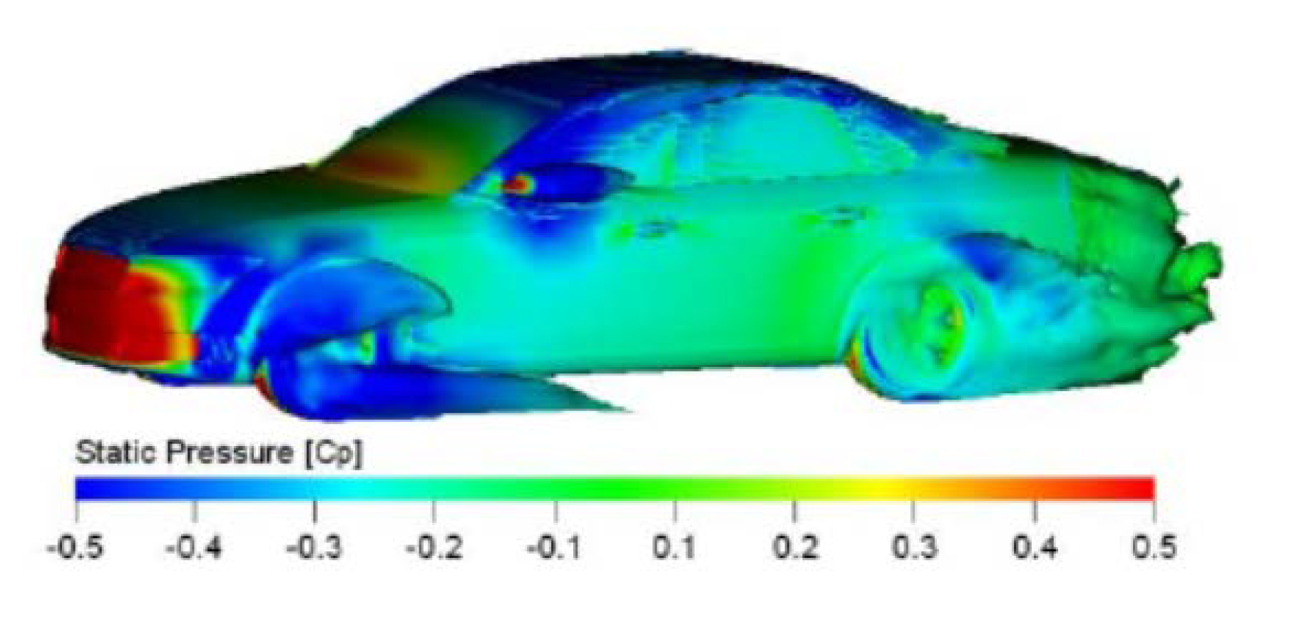
The static pressure distributions on the side window area under two different methods are displayed in Figure 14 and Figure 15. The positive pressure area is on the windward side of the rearview mirror, while the negative one is located on the A-pillar, rim of the rearview mirror frame, and core area of the rearview mirror tail. Airflow separates after passing through the rearview mirror, forms turbulent vortices in the wake core of the rearview mirror, and develops along the rear of the rearview mirror. Turbulent vortices exhibit intermittent shedding. Therefore, pressure fluctuation in the tail space of the side window region is intensified.
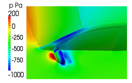
Figure 14.
Pressure contour obtained using the SLM method at t = 0.765 s.

Figure 15.
Pressure contour obtained using the DSLM method at t = 0.765 s.
The velocity distribution and pressure contour of DSLM is similar with those of SLM. The empirical coefficient is constant for the SLM model but dynamic for the DSLM model. The flow fields of two models are similar, but the values are different.
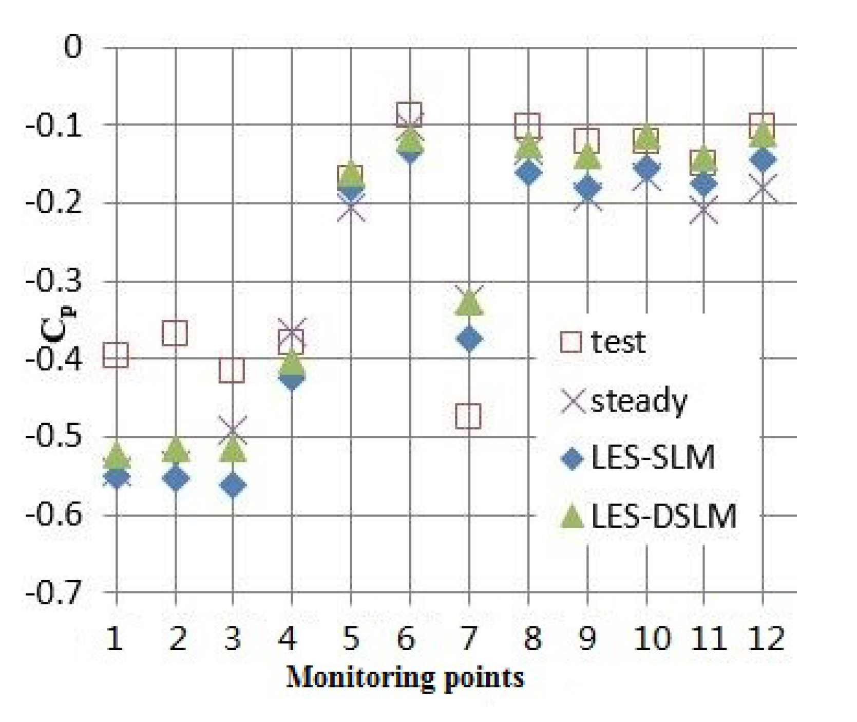
The pressure coefficients (Cp) of the monitoring points on the side window are obtained and compared with the test results. The pressure coefficients are averaged by the flow field time. The period of vortex shedding at the rearview mirror tail is approximately 0.05 s, and the pressure coefficients are obtained by averaging the integral of the pressure fluctuation periods. Figure 16 reveals some errors between the simulation and test results at points 1, 2, 3, and 7. The maximum difference between the simulation and test results is approximately 25%. However, the other monitoring points exhibited good consistency, and the overall trend of the values along the x-axis is the same.
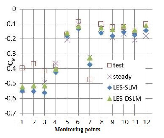
Figure 16.
Comparison between pressure coefficients obtained using simulation and test.
By contrast, the simulation results of DSLM are closer to the test results compared with those of SLM, so the DSLM subgrid model is more suitable to simulate the flow field of vehicle. This finding suggests that the proposed method can accurately simulate the turbulent boundary layer flow in the reattachment zone.
5.2. Analysis of the Sound Field
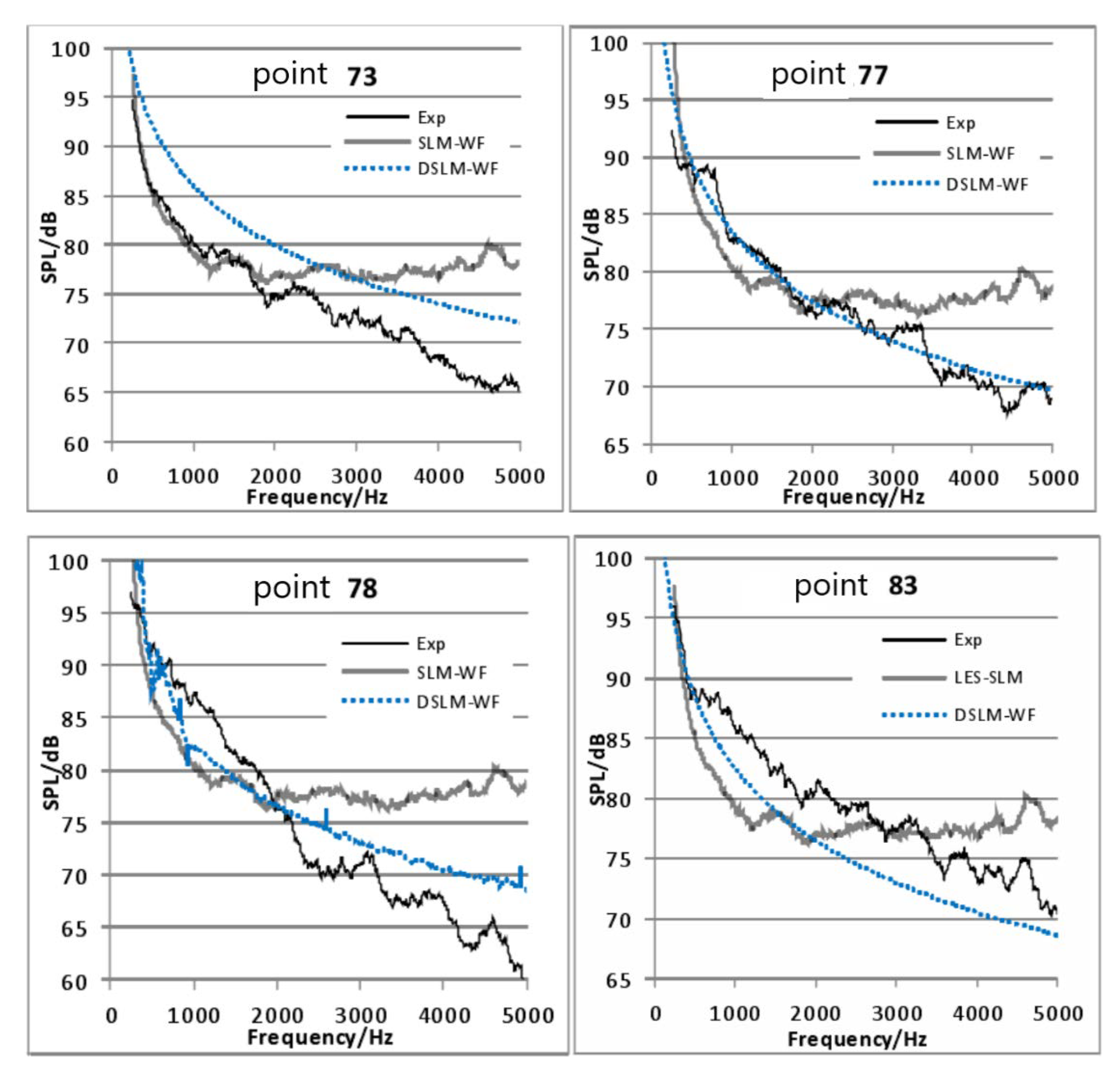
The sound pressure level curves of the monitoring points on the side window are obtained using LES of the different subgrid models with the wallfunction. The results are compared with the test results (Figure 17). In the middle and high-frequency bands, the sound pressure level curve of the DSLM subgrid model is closer to the test results compared with that of the SLM sub-grid model. The sound pressure levels in the DSLM subgrid model and wind tunnel test demonstrate a downward trend in the entire frequency domain. The sound pressure level curve obtained by the SLM subgrid model maintains a horizontal trend in the middle and high-frequency bands (1000–5000 Hz). These results differ from the trend observed in the test.
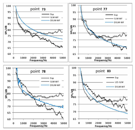
Figure 17.
Sound pressure levels on the front side window obtained in the simulation and test.
The results of the DSLM-WF show that the maximum difference is approximately 10dB. Moreover, the majority of the monitoring points are located in the core area of the rearview mirror wake, which is affected by the wake turbulence vortex. The intermittent knocking on the side window makes the surface pressure fluctuate violently, which is a difficulty in simulation experiments that affects the accuracy of the numerical simulation results to some extent. However, the trend of the simulation and test results in the entire frequency domain was identical, thereby implying the need to further investigate the noise in this area.
5.3. Analysis of Simulation Results
The velocity distributions in the cross-section obtained by the DSLM method at different times are illustrated by the plane at z = 1.12 m in the wake region of the rearview mirror. The characteristics of the flow field in this region are subsequently analyzed (Figure 18). The vortices behind the rearview mirror are shedding intermittently, with a shedding period of approximately 0.05 s.
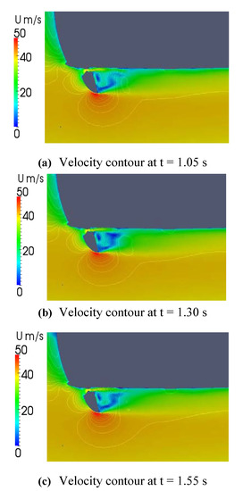
Figure 18.
Velocity distribution in the cross-section obtained using DSLM at z = 1.12 m.
The velocity distributions show that two rotating vortices are present in the low-speed region of the rearview mirror wake, and the motion direction of both vortices opposes each other. Airflow accelerated after flowing through the gap between the rearview mirror and side window, thereby forming a clockwise vortex. The other part of the airflow was accelerated after flowing through the outer edge of the rearview mirror, thereby forming a counterclockwise vortex. The inside airflow with high velocity impacted the side window and intensified the pressure fluctuation, thereby producing aerodynamic noise.
The cause of aerodynamic noise is explained by the global flow field. It is the isosurface map of the vehicle body surface as shown in Figure 19. It can be seen from the figure that there are low frequency and large size turbulence vortices at the wheels and wake, especially at the A pillar and rearview mirror. It indicates that there are air separation and energy loss in these places. This can be verified in Figure 20, which shows the velocity pulsation behind rearview mirror.

Figure 19.
Isosurface map of vehicle surface when total pressure is zero.
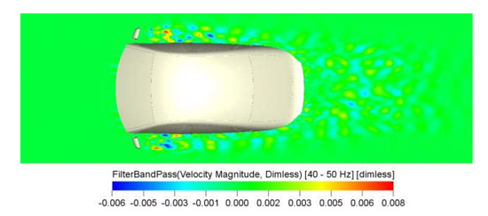
Figure 20.
Velocity pulsation on horizontal section.
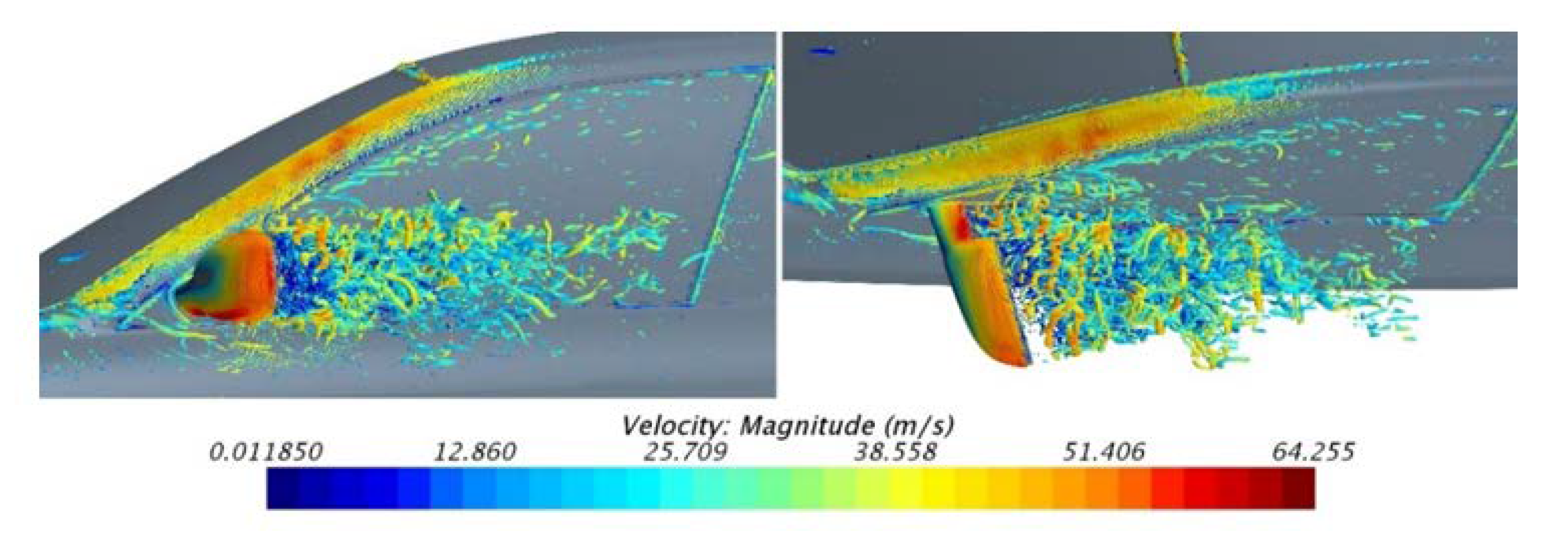
The isosurface map of Q criterion around mirror area is shown as Figure 21, which is rendered with the speed value. From side view and top view, it can be seen that the A-pillar vortices formed after the air flows through the A-pillar from the front windshield and the wake vortices structure of the rear-view mirror. These vortices interfere each other and develop dissipation at all times. The vortices act on the side window, resulting in strong pressure fluctuation, which caused the aerodynamic noise.
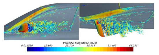
Figure 21.
Isosurface map of Q criterion (side view and top view).
6. Conclusions
The flow field around vehicle and the aerodynamic noise could be obtained by LES method. The simulation results using the DSLM model are more accurate than those using SLM model. The results of DSLM model are closer to the results of wind tunnel test, so the method of DSLM is more suitable to simulate aerodynamic noise of vehicle.
During the course of flowing through the A-pillar to the side window, the airflow separated and formed a turbulent region thereafter. After the separation, some airflow attached to the side window and top beam. The airflow passing through the rearview mirror separated. The lower part of the airflow reattached to the side window region, and the vortex structures in this area are extremely complex. The velocity distributions in the cross-section at z = 1.12 m showed that two opposite vortices are formed in the low-speed region of the rearview mirror wake. Thus, the faster inner airflow produced an impact on the side window. The turbulent vortices in this area intermittently shed and the pressure fluctuation on the side window substantially changed, which is the source of the aerodynamic noise.
Author Contributions
Conceptualization, X.H.; Writing—original draft, P.G.; Resources, Z.W.; Data curation and Supervision, J.W.; Writing—review and editing, M.W.; J.Z.; D.W. All authors have read and agreed to the published version of the manuscript.
Funding
This work was supported by the National Science Foundation of China (No. 51875238).
Acknowledgments
I would like to express my gratitude to all those who helped me during the writing of this paper. I gratefully acknowledge the help of staff of the wind tunnel laboratory of Jilin University who has offered me the necessary assistance in the academic studies.
Conflicts of Interest
The authors declare no conflict of interest.
References
- Yang, Z.D.; Gu, Z.Q.; Xie, C.; Zong, Y.Q.; Jiang, C.M. Experimental research on noise reduction mechanism of a groove spoiler in vehicle sunroof. J. Hunan Univ. (Nat. Sci.) 2018, 45, 26–34. [Google Scholar]
- Robert Powell, Sivapalan Senthooran and Philippe Moron. A Computational Process to Effectively Design Seals for Improved Wind Noise Performance; SAE Paper, 2019-01-1472; SAE: Warrendale, PA, USA, 2019. [Google Scholar]
- Hu, X. Automotive Aerodynamics; China Communications Publishing: Beijing, China, 2014. [Google Scholar]
- Gu, Z. Automotive Aerodynamics; China Communications Publishing: Beijing, China, 2005. [Google Scholar]
- Tadakuma, K.; Sugiyama, T.; Maeda, K. Development of Full-Scale Wind Tunnel for Enhancement of Vehicle Aerodynamic and Aero-Acoustic Performance; SAE Paper, 2014-01-0598; SAE: Warrendale, PA, USA, 2014. [Google Scholar]
- Terakado, S.; Makihara, T.; Sugiyama, T.; Maeda, K.; Tadakuma, K.; Tsuboi, K. Experimental Investigation of Aeroacoustic Cabin Noise in Unsteady Flow by Means of a New Turbulence Generating Device; SAE Paper, 2017-01-1545; SAE: Warrendale, PA, USA, 2017. [Google Scholar]
- Iacovoni, D.P.; Zeuty, E.J.; Morello, D.A. Wind Noise and Drag Optimization Test Method; SAE Paper, 2003-01-1702; SAE: Warrendale, PA, USA, 2003. [Google Scholar]
- Khalighi, B.; Johnson, J.P.; Chen, K.; Lee, R.G. Experimental Characterization of the Unsteady Flow Field behind Two Outside Rear View Mirrors; SAE Paper, 2008-01-0476; SAE: Warrendale, PA, USA, 2008. [Google Scholar]
- Yang, B. Research on Automobile Exterior Aerodynamic Noise [D]; Jilin University: Changchun, China, 2008. [Google Scholar]
- Li, W.; Liu, N.; Wang, Y.; Guo, H. Contribution Analysis of Noise on Driver’s Ear Side of High Speed Vehicles. Noise Vib. Control 2019, 1, 24–28. [Google Scholar]
- Itoh, A.; Wang, Z. The Mechanism of Hissing Noise in the Automotive Cabin and Countermeasures for Its Reduction; SAE Paper, 2019-01-1474; SAE: Warrendale, PA, USA, 2019. [Google Scholar]
- Yang, J.; Zhang, S.; Dong, G.; Jiang, H. Research on Frequency Characteristics of Automobile Interior Wind Noise in Wind Tunnel Test. Chin. J. Automot. Eng. 2019, 6, 445–451. [Google Scholar]
- Sovani, S.D.; Chen, K.-H. Aero Acoustics of an Automotive A-Pillar Raingutter: A Numerical Study with the Ffowcs-Williams Hawkings Method; SAE Paper, 2005-01-2492; SAE: Warrendale, PA, USA, 2005. [Google Scholar]
- Islam, M.; Decker, F.; de Villiers, E.; Jackson, A.; Gines, J. Application of Detached–Eddy Simulation for Automotive Aerodynamics Development; SAE Paper, 2009-01-0333; SAE: Warrendale, PA, USA, 2009. [Google Scholar]
- Krajnovic, S. Exploration and Improvement of Road Vehicle Aerodynamics Using LES; SAE Paper, 2011-01-0176; SAE: Warrendale, PA, USA, 2011. [Google Scholar]
- Li, Q.; Du, W.; Wang, Y.; Yang, Z. Aerodynamic Noise Control of Automobile Rear View Mirror Based on Active Jet. J. Tongji Univ. (Nat. Sci.) 2019, 8, 1195–1200. [Google Scholar]
- Jiang, H.; Lai, W.; Zhang, S.; Dong, G.; Jia, W.; Pang, J. Research on Aeroacoustic Optimization of Vehicle Rearview Mirror. Automot. Eng. 2020, 42, 121–126. [Google Scholar]
- Yang, B.; Hu, X.J.; Zhang, Y.C. Study on unsteady flow field and aerodynamic noise of automotive rear view mirror region. J. Mech. Eng. 2010, 46, 151–155. [Google Scholar] [CrossRef]
- Wang, J.; Chen, R.; Yang, J.; Gong, X.; Li, L. Simulation and Experimental Study on Aerodynamic Noise of Automotive Pear-view Mirror. Automot. Eng. 2018, 40, 1480–1486. [Google Scholar]
- Xiao, H.L.; Luo, J.S. Improvement of sub-grid model in large eddy simulation and applications in turbulent channel flow. J. Aerosp. Power 2007, 22, 583–587. [Google Scholar]
- Khalighi, B.; Chen, K.H.; Johnson, J.P.; Snegirev, A.; Shinder, J.; Lupuleac, S. Computational and experimental investigation of the unsteady flow structures around automotive outside rear-view mirrors. Int. J. Automot. Technol. 2013, 14, 143–150. [Google Scholar] [CrossRef]
- Piscaglia, F.; Montorfano, A.; Onorati, A. Towards the LES simulation of IC engines with parallel topologically changing meshes. J. Biol. Chem. 2013, 6, 926–940. [Google Scholar] [CrossRef]
- Serre, E.; Minguez, M.; Pasquetti, R.; Minguez, M.; Deng, G.B. On simulating the turbulent flow around the Ahmed body: A French–German collaborative evaluation of LES and DES. Comput. Fluids 2013, 78, 10–23. [Google Scholar] [CrossRef]
- Biswas, K.; Gadekar, G.; Chalipat, S. Development and Prediction of Vehicle Drag Coefficient Using OpenFoam CFD Tool; SAE Paper, 2019-26-0235; SAE: Warrendale, PA, USA, 2019. [Google Scholar]
- Wang, F.J. Computational Fluid Dynamics Analysis, 3rd ed.; Tsinghua University Press: Beijing, China, 2004. [Google Scholar]
- Lilly, D.K. A proposed modification of the germano subgrid-scale closure model. Phys. Fluids 1992, 4, 633–635. [Google Scholar] [CrossRef]
- Germano, M.; Piomelli, U.; Moin, P.; Cabot, W.H. Dynamic Subgrid-Scale Eddy Viscosity Model. In Summer Workshop; Center for Turbulence Research: Stanford, CA, USA, 1996. [Google Scholar]


© 2020 by the authors. Licensee MDPI, Basel, Switzerland. This article is an open access article distributed under the terms and conditions of the Creative Commons Attribution (CC BY) license (http://creativecommons.org/licenses/by/4.0/).