Abstract
Superheated steam temperature (SST) is a significant index for a coal-fired power plant. Its control is becoming more and more challenging for the reason that the control requirements are stricter and the load command changes extensively and frequently. To deal with the aforementioned challenges, previously the cascade control strategy was usually applied to the control of SST. However, its structure and tuning procedure are complex. To solve this problem, this paper proposes a single-loop control strategy for SST based on a hybrid active disturbance rejection control (ADRC). The stability and ability to reject the secondary disturbance are analyzed theoretically in order to perfect the theory of the hybrid ADRC. Then a tuning procedure is summarized for the hybrid ADRC by analyzing the influences of all parameters on control performance. Using the proposed tuning method, a simulation is carried out illustrating that the hybrid ADRC is able to improve the dynamic performance of SST with good robustness. Eventually, the hybrid ADRC is applied to the SST system of a power plant simulator. Experimental results indicate that the single-loop control strategy based on the hybrid ADRC has better control performance and simpler structure than cascade control strategies. The successful application of the proposed hybrid ADRC shows its promising prospect of field tests in future power industry with the increasing demand on integrating more renewables into the grid.
1. Introduction
With the continuous increase of the power demand and the development of renewable energy in the electricity market, power plant control remains a challenging problem [1]. By 2040, the global net generation is predicted to increase at a rate of 2.2% annually [2]. As a result, the utilization of renewable energy such as solar, wind power and hydropower are anticipated to increase by 2.8% per year in order to alleviate the dependency on the consumption of fossil fuel [2]. When the time comes, the renewable energy generation will account for quarter of the total generation in the world. However, the randomness and intermittency of renewable power bring huge challenges to the stability and reliability of the grid [3]. One of the feasible solutions to solve this problem is accelerating the respond speed of automatic generation control (AGC) in power plants.
Superheated steam temperature (SST) is regarded as a vital parameter in the daily operation of a coal-fired power plant. The superheater and the high-pressure components of the steam pipelines could be damaged if the SST is beyond its upper limit. On the other hand, if the SST is lower than its lower limit, the power generation efficiency would decrease which may influence the economical operation of the turbines. Therefore, most researchers recommended that SST should be in the range of ±5 °C of its set point [4]. The significance of the control of SST is to ensure the units work safely and efficiently. Generally, in terms of subcritical units, the SST of most power plants should remain within a 530 °C to 545 °C range.
Since the SST is a typical thermal process with great inertia and large delay, a cascade control structure is commonly applied to the SST. Proportional-integral (PI) controllers are chosen as the inner-loop controllers while proportional-integral-derivative (PID)/PI controllers are chosen as the outer-loop controllers. However, when the working conditions change widely, the conventional PI cascade control of SST is not able to achieve satisfactory control performance with the limit of PI controller [5]. Consequently, many advanced and improved control strategies were proposed to handle the control difficulties such as model predictive control (MPC) [6], neural network [7], fuzzy control [8] and fractional order proportional integral differential (FOPID) control [9]. Although these control strategies are able to obtain satisfactory control performance in simulation experiments, they are rarely used in a practical unit due to following reasons:
- Some advanced controllers should be designed based on the accurate mathematical model of SST. However, it is difficult to obtain the accurate mathematical description of SST for the reason that the characteristics of SST changes with the working conditions.
- Because of their complexities in computation, most of advanced strategies are unable to be implemented on the distributed control system (DCS) of a power plant.
In addition to SST, many industrial processes cannot be described by explicit mathematical models. Therefore, the controllers, which are designed not based on models, play an important role in modern industry. In terms of the tower crane system, the model-free adaptive control (MFAC) [10] are applied to it combined with fuzzy component [11]. This application shows the promising prospect of the model-free controller.
Active disturbance rejection control (ADRC), proposed by the Chinese scholar Han, is regarded as the successor of PID controller in the control synthesis of modern industry [5]. Its core idea is that uncertainties, modeling error and external disturbances are considered as an extended state in total which is able to be estimated and compensated actively by the extended state observer (ESO) [12]. In addition, ADRC inherits the advantages of PID and has less dependency on the accurate models of processes. However, ADRC was first proposed in a nonlinear form which makes its implementation on DCS complex as well. In order to solve this problem, Gao simplified the nonlinear ADRC into the linear form and proposed its tuning procedure based on the bandwidth-parameterization [13]. This simplification lays a foundation for the field application of ADRC. In recent years, the linear ADRC is widely used to solve problems in engineering, especially in the control of thermodynamic objects such as circulating fluidized bed (CFB) boilers [14], waste heat recovery systems [15], gasifiers [16], nuclear heating reactor [17], secondary air flow [18], proton exchange membrane fuel cell [19,20], vibration suppression [21] and heavy-duty diesel engine [22]. These applications show the developing prospects of ADRC in industry.
Actually, the ability of ADRC to control a high-order system is limited, particularly its response in reference tracking is slow even if it has advantages in disturbance rejection [4]. Moreover, the control structure of SST based on ADRC is cascade which means the structure of SST control system is complicated. In this paper, a hybrid ADRC is proposed in order to simplify the control structure and enhance the control performance on SST. Note that the control of SST based on the hybrid ADRC is a single-loop control system. Following are the main achievements of this paper:
- A hybrid ADRC is proposed in order to simplify the control structure of the conventional SST control system.
- The stability of the hybrid ADRC is analyzed theoretically. Moreover, the ability of disturbance rejection of the hybrid ADRC is discussed in this paper.
- The tuning procedure of the hybrid ADRC is summarized based on the influences of its parameters on control performance.
- The hybrid ADRC has been applied to a power plant simulator successfully. Its control performance is validated by the running data.
The rest of this paper is organized as follows: The next section briefly introduces the SST model and the regular cascade control strategy. Combined with the regular ADRC design, the proposed hybrid ADRC is introduced in Section 3 and followed by the stability analysis and the discussion of ability to reject the disturbance. Section 4 provides a tuning procedure of the hybrid ADRC and illustrates its control performance by a numerical simulation. In Section 5, the proposed hybrid ADRC is applied to the SST control system of a power plant simulator and results show its advantages in tracking and disturbance rejection. Eventually, concluding remarks are offered in the last section.
2. The SST System and Its Regular Control
2.1. SST Model Description
Figure 1 shows the schematic diagram of the power plant superheater system which consists of two superheaters, including the 1st stage superheater and the 2nd stage superheater. Steam from the drum or the steam separator flows through desuperheaters and superheaters during which it absorbs heat from the flue gas. Water spray is the main method to control SST in most power plants [23]. The water in attemperator is extracted from an intermediate stage of the boiler feed water pump [24].
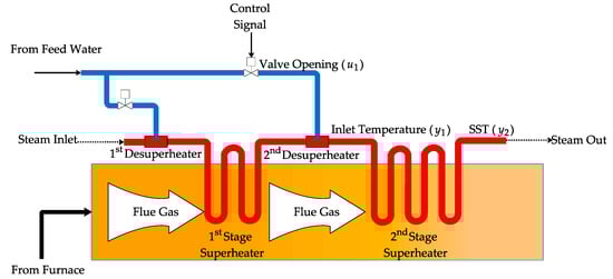
Figure 1.
The schematic diagram of SST system in a power plant.
In general, it is difficult to establish the accurate mechanism model of SST so that transfer functions are commonly used to describe the dynamics in SST system. In this paper, we define u1, y1 and y2 as the opening of valve, the inlet temperature and the outlet temperature of 2nd stage superheater, respectively. Therefore, transfer functions from u1 to y1 and from y1 to y2 are depicted as follows:
where G1(s) and G2(s) represent the transfer functions of the leading segment and the inertia segment, respectively. K1 and T1 are dynamic parameters of G1(s) while K2 and T2 are those of G2(s). These dynamic parameters are able to be obtained by system identifications. n1 and n2 are the orders of G1(s) and G2(s) which are usually given as 2 and 4, respectively. Based on the aforementioned description the control difficulties of SST can be summarized as follows:
- An accurate mathematical model of SST is unavailable.
- High order dynamics of the 2nd superheater results in a slow response to the set point and disturbances.
- Various disturbances such as load demand, combustion air flow and main steam flow have significant adverse impacts on SST.
A coal-fired power unit usually operates in the wide load range of 50–100% and the load command is regulated frequently. It means that the characteristics of SST varies drastically with the change of the working condition. To handle with model uncertainties, the closed-loop control system should be robust enough.
2.2. Regular Control Structure of SST
Because of the sluggish response of the 2nd stage superheater, the cascade control structure shown in Figure 2 is usually chosen for the SST control system of a power plant, where G1(s) is defined as the inner-loop transfer function and G2(s) is denoted as the outer-loop transfer function.
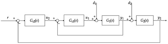
Figure 2.
The block diagram of SST cascade control system.
In Figure 2, Gc1(s) and Gc2(s) represent the inner-loop controller and outer-loop controller, respectively. The set point r is denoted as the desired SST. Moreover, the output of Gc2(s) is designed as the set point of the inlet temperature y1.
The inner-loop disturbances, defined as d1, consist of the pressure and temperature change of spray water which are modeled as a step response. Similarly, the outer-loop disturbances, denoted as d2, include load variation, combustion instability and the coal quality variation which can be considered as another step response. d1 and d2 are defined as the secondary disturbance and the primary disturbance of the SST system, respectively. However, the conventional cascade control system has been criticized for its complex structure and tuning procedure [25]. Consequently, a hybrid ADRC is proposed to solve these problems.
3. Hybrid Active Disturbance Rejection Control
3.1. Regular Design of ADRC
In this paper, we take the first order ADRC as an example. Suppose that the controlled object is able to be considered as a general first order system:
where is the synthesis of external disturbances, high order dynamics and modelling uncertainties of the general first order system. u is denoted as the input of the system while y is defined as the output of the system. b represents the critical gain [24], whose value may be unknown for a process.
We rewrite Equation (3) as follows:
where b0 is the estimation of b and f is defined as the total disturbance of the system which can be derived as:
Typically, the state vector of a first order system is depicted as x = [y], which only consists of one state variable. Let x2 = f, where is x2 is known as the extended state of the system.
Define the state vector x as:
Therefore, the state space expressions of Equation (4) can be depicted as,
where , , and .
The ESO is designed for the system as:
where z = [z1 z2]T represents the state vector of ESO and L = [β1 β2]T is the gain vector of the observer. If β1 and β2 are tuned reasonably, z is able to track x accurately [26].
The state feedback control law (SFCL) is designed as:
where r = [r dr/dt]T and r is denoted as the reference signal. It should be noted that dr/dt is equal to zero if r is unbounded [4]. K= [kp / b0 1/ b0] is defined as the gain vector of the controller.
In order to simplify the tuning procedure of ADRC, Z. Gao proposed a tuning method based on bandwidth-parameterization [13]. ωc and ωo are defined as the bandwidth of the closed-loop control system and the observer, respectively. The gain vector of ESO is set as [2ωo ωo2]T so that all eigenvalues of A-LC are placed at −ωo. Likewise, K is set as [ωc / b0 1/ b0] to ensure that all eigenvalues of à are placed at -ωc, where à is able to be depicted as:
Therefore, in terms of the first order ADRC, its parameters are able to be given as:
In addition, b0 is also a tunable parameter of ADRC. The block diagram of first order ADRC is shown in Figure 3.
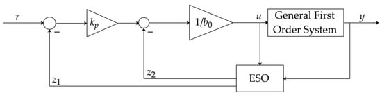
Figure 3.
The block diagram of a 1st order ADRC.
The general first order system in Figure 3 is depicted using Equation (3).
3.2. Hybrid ADRC Design for SST System
Designed based on the conventional cascade structure, the SST control system is able to track the reference signal rapidly and has a strong ability of disturbance rejection. However, as mentioned above, the structure of a cascade control system is complicated, which brings difficulties to its configuration on the platform of DCS. Moreover, using a cascade control strategy, the output of SST system fluctuates fiercely when the secondary disturbance exists. In this subsection, a hybrid ADRC is proposed based on the regular first order ADRC to simplify the control structure of a SST system and steadily reject the secondary disturbance. Besides, this single-loop control strategy should obtain better control performance than that of the cascade control strategy.
Transfer functions of an SST system can be depicted as Equations (1) and (2). The block diagram of SST system based on the hybrid ADRC is illustrated in Figure 4.
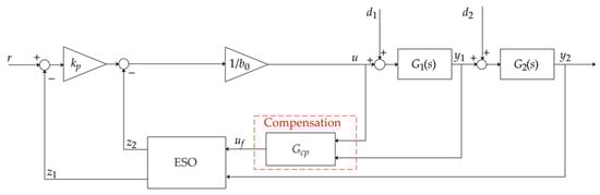
Figure 4.
The hybrid ADRC designed for an SST system.
Compared with the regular first order ADRC, the hybrid ADRC adds a compensation part before the control signal goes into ESO. uf is defined as the compensated control signal. Differential equations of Gcp are depicted as:
where z3 is denoted as an intermediate variable of the compensation part. β3 and b1 are defined as the tunable parameters of Gcp. It is obvious that the compensation part is designed based on the reduced-order ESO which is the equivalence of first order ESO [27]. Since ESO has the ability of compensation and estimation, uncertainties and disturbances between u and y1 are able to be compensated and estimated by Gcp, which means that the hybrid ADRC can reduce the dynamic deviation caused by d1 effectively.
Similar with the regular first order ADRC, the ESO of the hybrid ADRC is designed as:
The SFCL of the hybrid ADRC is the same with Equation (9). Obviously, the hybrid ADRC inherits the simple structure of regular ADRC so that it is easy to be implemented on DCS.
3.3. Analysis of Hybrid ADRC
In this subsection, the stability is analyzed and ability to reject the secondary disturbance of the hybrid ADRC is discussed. Moreover, the proof and discussion are given as well.
3.3.1. Stability Analysis
Theorem 1.
The closed-loop system is stable if all roots of Equation (26) are on the left half-plane.
Proof of Theorem 1.
G1(s) and G2(s) are able to be considered as general first order systems as depicted in Equation (3):
where g1 and g2 are the syntheses of external disturbances, high order dynamics and modelling uncertainties of two objects. Their critical gains, defined as b and
in this subsection, are unknown so that Equation (14) can be rewritten as:
where b1 is known as the tunable parameter of the compensation part, which is able to be regarded as the estimation of b; b2 is denoted as the estimation of
which is able to be obtained by the result of model identification. Besides, f1 and f2 are defined as total disturbances of two objects which can be derived as:
As for the compensation part, its expressions on s-plane are able to be depicted as:
Therefore, Equation (18) can be rewritten as:
Combined with Equation (15), it is evident that:
Let the tracking errors be and , then it is obvious that and . As a result, differential equations of ESO can be written as:
Moreover, the SFCL can be depicted as:
Based on Equation (15), (20)–(22), the closed-loop system is able to be summarized as:
where and . Besides, Λ and Ψ can be derived as follows:
Then characteristic equation of the closed-loop system is able to be derived by the following expression:
If all roots of Equation (26) are on the left-half plane, the system is stable. □
Remark 1. Routh-Hurwitz Criterion:
The necessary and sufficient condition of the stability of linear systems is that all elements in the first column of Routh array are greater than zero [28].
According to Remark 1, the system is stable if parameters of the hybrid ADRC satisfy following conditions:
3.3.2. Rejection of the Secondary Disturbance
As mentioned in Section 3.2, the hybrid ADRC has a strong ability to eliminate the dynamic deviation caused by the secondary disturbance d1. In this subsection, its ability to reject d1 is discussed based on the equivalence of the block diagram of the system as shown in Figure 4.
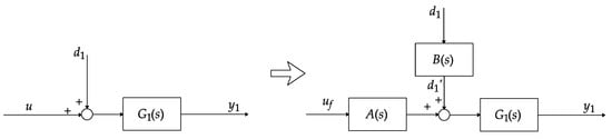
Figure 5.
The equivalence from u to y1.
According to Equation (18), the transfer functions of A(s) and B(s) can be derived as:
If |b1| is sufficiently small, it is obvious that . Then D1’(s) << D1(s). Therefore, we are able to conclude that with the decrease of |b1|, the dynamic deviation caused by d1 is smaller. This conclusion will be validated in the next section.
Figure 6 shows the equivalent structure of the closed-loop system. In order to illustrate that the hybrid ADRC enables to reject the secondary disturbance, we first derive the transfer function from d1 to y2.
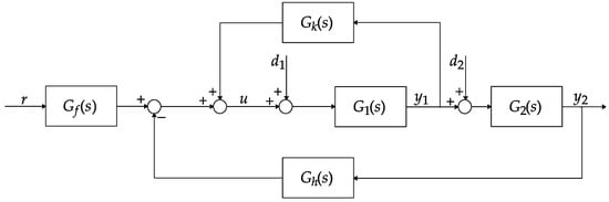
Figure 6.
The equivalent block diagram of the closed-loop system.
Let and , then we have , and .
Based on Mason’s signal-flow gain formula, the transfer function from d1 to y2 is derived as:
Then Equation (33) can be approximated under the low frequency:
In terms of low-frequency disturbances, Equation (34) means that the hybrid ADRC has a strong ability of disturbance rejection. Note that secondary disturbances of the aforementioned SST system are usually low-frequency disturbances.
4. Tuning Procedure and Numerical Simulation
4.1. Tuning Procedure of Hybrid ADRC
To summarize the procedure of hybrid ADRC, we first study on the influences of its parameters on the control performance. Consider the SST model provided in [29]:
This model is identified to describe the SST of Hongshan power plant simulator in the research institute of Fujian Histron. The model is identified at about 70% load. The initial parameters of the hybrid ADRC are set as: ωc = 0.05, b0 = −0.18, ωo = 0.2, b1 = −0.026, β3 = 4. One of them will change while others remain unchanged. The influences of different parameters on the control performance are shown in Figure 7, Figure 8, Figure 9, Figure 10 and Figure 11.
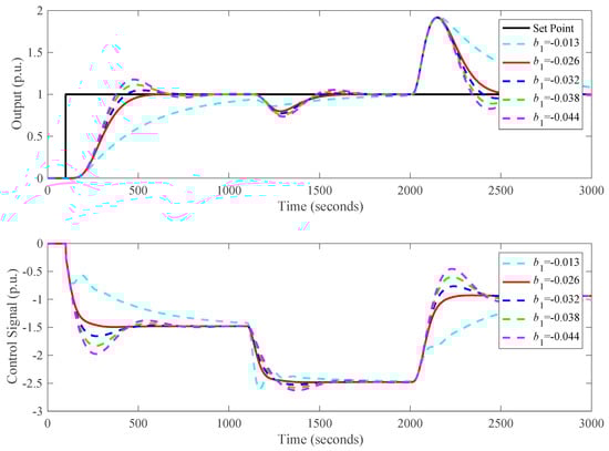
Figure 7.
The influences on control performance with different b1.

Figure 8.
The influences on control performance with different β3.
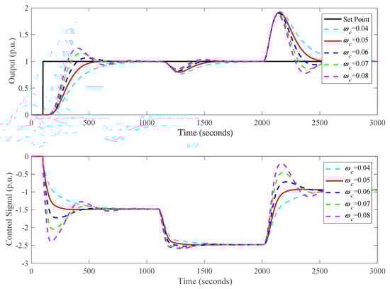
Figure 9.
The influences on control performance with different ωc.
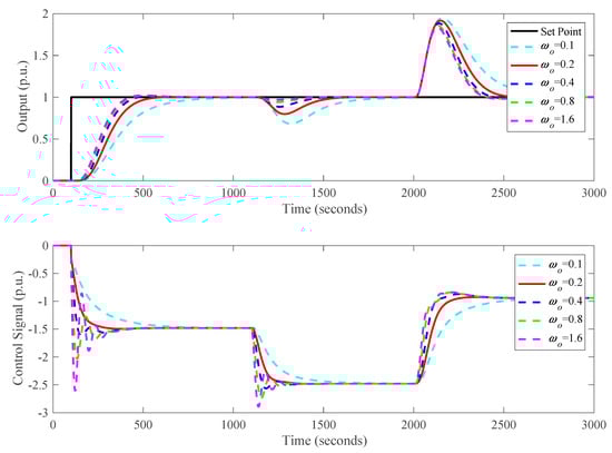
Figure 10.
The influences on control performance with different ωo.
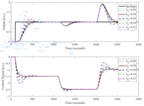
Figure 11.
The influences on control performance with different b0.
- b1 is negative because it represents the estimation of the critical gain of G1(s). The smaller |b1| means a slower tracking speed, weaker dynamic deviation caused by the secondary disturbance and worse performance of rejecting the primary disturbance. However, |b1| should not decrease infinitely for the reason that the control signal will oscillate significantly which may lead to irreversible damage to the actuator.
- The increases of β3 and ωo will improve the control performance of the closed-loop system. Moreover, it is obvious that the output has no obvious change when they are big enough.
- With the increase of ωc, the control effect of the hybrid ADRC will be enhanced. Besides, the larger ωc means a greater overshoot.
- b0 decides the positive-negative action of the hybrid ADRC. In terms of the SST system, b0 is negative for the reason that SST is able to be regarded as a negative process in general. Contrary to ωc, the smaller |b0| means stronger control effect of the hybrid ADRC. In addition, its decrease will augment the overshoot.
Based on the influences of parameters of the hybrid ADRC on the control performance, a practical tuning procedure can be summarized as follows:
- First of all, b1 and b0 should be fixed. b1 is recommended to set in the range (−∞,] while b0 is suggested to set in the range (−∞,].
- Set a small ωc. Then augment β3 and ωo to proper values until the output has no obvious change. Note that β3 and ωo are unable to increase infinitely in case that the control signal will oscillate fiercely.
- Augment ωc to a proper value until the overshoot and the settling time satisfy the control requirements.
- When the control performance is satisfactory, the tuning procedure terminates. Otherwise, repeat steps (1)–(3) as mentioned.
Eventually, the flow chart of the tuning procedure given in Figure 12 can be used to guide the tuning of the hybrid ADRC. The following are some recommendations of the tuning procedure:
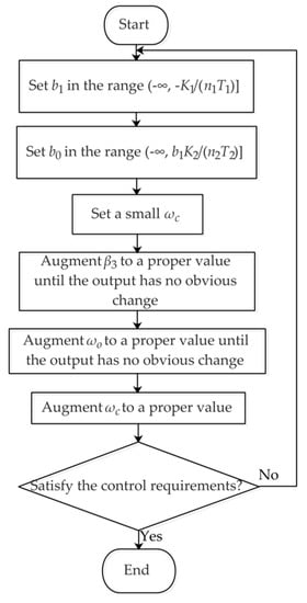
Figure 12.
Flow chart of the hybrid ADRC tuning.
- According to the stability analysis, values of β3 and ωo should be positive.
- The final values of b1 and b0 are far smaller than −K1/(n1T1) and b1K2/(n2T2), respectively. In addition, during the tuning procedure, b1 and b0 are recommended to be tuned as the integral multiple of −K1/(n1T1) and b1K2/(n2T2), respectively.
- The initial value of ωc is recommended to set in the range [0.01, 0.1].
- The bandwidth of ESO ωo is recommended to be tuned as 3–10ωc in order to let the output has no obvious change.
4.2. Numerical Simulation
In order to embody superiorities of the hybrid ADRC, we carried out a numerical simulation. Most of control systems have regular single-loop control structures. However, the normal single-loop control strategies are unable to weaken the dynamic deviation caused by the secondary disturbance and quicken the tracking response in terms of the control of SST. Therefore, cascade control is usually chosen as the control strategy of SST for the reason that it has three advantages [30]:
- It provides faster action to reduce the disturbance in inner loop;
- It improves the response rate and control accuracy for large lag systems;
- It reduces the effect of parameter variations in inner loop.
Consequently, in this paper, the cascade control strategies are selected as the comparative control strategies of the hybrid ADRC.
Consider the SST system depicted as Equation (35). In this subsection, the proposed hybrid ADRC is compared with control strategies which are mentioned in [30] such as PI-PI, ADRC-PI and the modified ADRC(MADRC)-PI. All parameters of different control strategies are listed in Table 1.

Table 1.
Parameters of different control strategies for numerical simulation.
According to [29], OPI-PI represents the original PI-PI cascade control strategy in the simulator; IPI-PI represents the improved PI-PI cascade control strategy optimized by genetic algorithm. Note that parameters of the hybrid ADRC are tuned based on the method shown in Figure 12 and those of other cascade control strategies are offered in [29]. Figure 13 illustrates the control performance of different control strategies on the SST system. During the simulation, the set point has a unit change at 0 s and a negative unit secondary disturbance is added at 3000 s. Moreover, a positive unit primary disturbance is added at 6000 s.
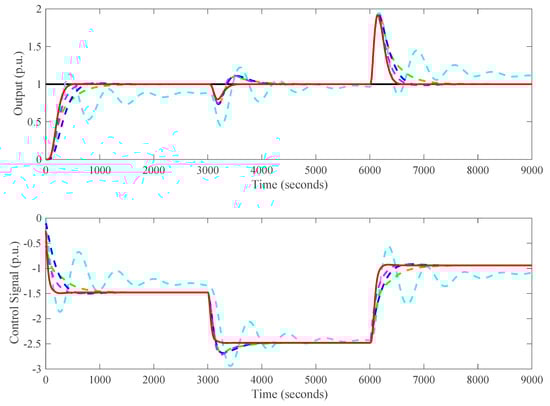
Figure 13.
The simulation results of different control strategies. (Set point: —, OPI-PI:- - -, IPI-PI: - - -, ADRC-PI: - - -, MADRC-PI: - - -, Hybrid ADRC: —).
In Figure 13, it is obvious that the hybrid ADRC is able to reject the secondary disturbance steadily because the output has no positive peak when d2 is added to the system. In terms of tracking performance, the proposed hybrid ADRC enables the output to track the set point faster than other cascade control strategies with hardly any overshoot. Moreover, it is able to reject the primary disturbance faster than other comparative control strategies.
For quantitative evaluation of dynamic performance, indices such as the overshoot (σ), the settling time (Ts) are calculated to indicate advantages of the hybrid ADRC as listed in Table 2. In addition, the integral absolute error (IAE) is chosen to evaluate the control performance of different control strategies comprehensively, which is depicted as:
where e(t) refers to the tracking error of the controlled variable. IAE tends to produce responses with less sustained oscillation [31]. IAEsp, IAEud2 and IAEud1 are denoted as the IAE of reference tracking, secondary disturbance rejection and primary disturbance rejection, respectively.
Table 2.
Dynamic indices of SST with different control strategies.
From Figure 13 and Table 2, it is evident that the hybrid ADRC has the best dynamic performance for the reason that its tracking is fastest and the overshoot is small enough. As for as the ability of disturbance rejection, the hybrid ADRC is best because it has the smallest IAEud2 and IAEud1.
Since the characteristics of SST change significantly with the working condition, the robustness of the hybrid ADRC is of importance. Monte Carlo trial is an effective method to test the robustness of a controller. In this subsection, the time constants and gains in Equation (35) are perturbed within a range of ± 10%. The simulation is repeated by 500 times for the perturbed system. Figure 14 shows the result of the Monte Carlo trials.
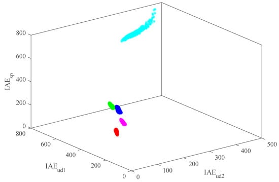
Figure 14.
Records of IAEsp, IAEud2 and IAEud1 for the perturbed system. (OPI-PI: *, IPI-PI: *, ADRC-PI: *, MADRC-PI: *, Hybrid ADRC: *).
Smaller indices mean the better dynamic performance. Moreover, if the scatter points are more intensive, the controller is more robust. In addition, the control strategy has better dynamic performance if its scatter points are nearer to the origin. In Figure 14, it is obvious that the scatter points of the hybrid ADRC are nearest to the origin and the most intensive. In order to evaluate the robustness of different control strategies quantitatively, we calculate the fluctuation range of IAEsp, IAEud2 and IAEud1.
According to Table 3, the hybrid ADRC has the narrowest ranges of IAEsp and IAEud2 but the range of IAEud1 of it is larger than those of IPI-PI, ADRC-PI and MADRC-PI. However, the range of IAEud1 of the proposed hybrid ADRC has the smallest upper-lower limit. Generally, the superiorities of the hybrid ADRC in tracking and disturbance rejection abilities have been validated.
Table 3.
Ranges of IAEsp, IAEud2 and IAEud1 of the perturbed system.
5. Field Application of the Hybrid ADRC on a Power Plant Simulator
5.1. The Model Identification Based on Multi-Objective Optimization
As mentioned in Section 2.1, the SST system is able to be approximated as a linear transfer function model which can be depicted as Equations (1) and (2). The orders of G1(s) and G2(s) are equal to 2 and 4, respectively.
In this subsection, the multi-objective genetic algorithm [32] is applied to optimize dynamic parameters such as time constants and gains. The optimization target is that the modeling errors of SST are minimum. The cost functions are defined as:
where m and Δt are denoted as the number of samples and the sampling interval. y1i and y1i d represent the i-th identified data and running data of G1(s), respectively; y2i and y2i d represent the i-th identified data and running data of G2(s), respectively.
The multi-objective genetic algorithm optimization is programmed by MATLAB. Its population size and the number of generations are 50 and 20, respectively. During the optimization, ranges of objectives are narrowing down in order to find the preferred solution. In this subsection, we expect γ1 and γ2 are small enough to satisfy the precision of model identification.
In this paper, we identified the SST system of a 150 MW power plant simulator whose load is about 66.7%. The optimization result is shown in Figure 15.
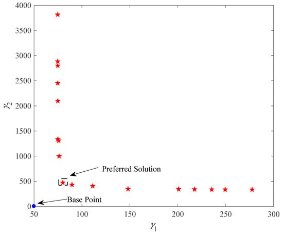
Figure 15.
Pareto fronts of model identification.
The computational time of model identification is 118.1886616s. Since γ1 and γ2 are denoted as modeling Errors in Equations (37) and (38), we can conclude that the solution point nearer to the based point has smaller modeling errors. According to Figure 15, the preferred solution point has the nearest distance to the base point which means that its modeling errors are smallest. As a result, it is regarded as the decision point. The identified SST models based on the decision point in Figure 15 are depicted as:
The comparison between the identified model and the real measurement is illustrated in Figure 16. It is obvious that the identified SST model is accurate enough for the design of control strategy.
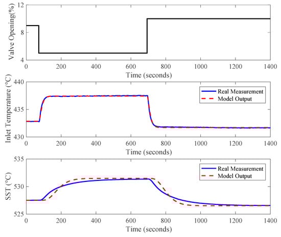
Figure 16.
The comparisons between the model output and the real measurement.
5.2. Field Application on a 150 MW Unit Simulator
5.2.1. Parameters of Control Strategies
Based on the SST models depicted as Equations (39) and (40), the proposed hybrid ADRC is designed for the SST system of the power plant simulator based on the tuning procedure summarized in Section 4.2. Besides, comparative control strategies are set as original PI-PI in the simulator (PIsim-PI), improved PI-PI (PIi-PI) and ADRC-PI. In Table 4, kp1 and ki1 are denoted as parameters of inner-loop PI controller. As for PIi-PI and ADRC-PI, parameters of their inner-loop controllers remain unchanged while those of their outer-loop controllers are optimized by the multi-objective genetic algorithm. The optimization targets are the settling time (Ts) and the IAE of tracking (IAEsp). In this subsection, the multi-objective genetic algorithm optimization is programmed by MATLAB as well. Similarly, the population size and the number of generations are set as 50 and 20, respectively. Figure 17 shows the parameter optimization results of ADRC-PI and PIi-PI. The computational time of parameter optimization of ADRC-PI and PIi-PI is 959.550412 s and 675.840116 s, respectively.
Table 4.
Parameters of different control strategies for SST system in the simulator.
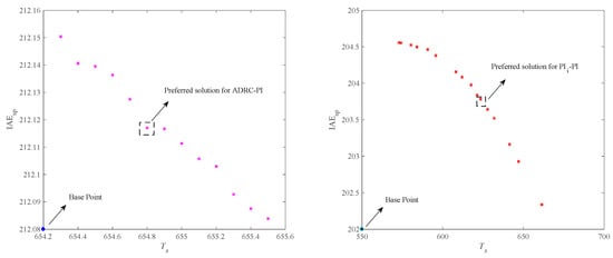
Figure 17.
The preferred solutions for parameters of ADRC-PI and PIi-PI.
5.2.2. Preliminary Numerical Simulations
The simulation is carried out to demonstrate the advantages of the proposed hybrid ADRC before it comes into service. During the simulation, the set point has a unit change at 100 s and a negative unit secondary disturbance is added at 1100 s. Moreover, a positive unit primary disturbance is added at 2000 s. Figure 18 illustrates the simulation results and dynamic indices are calculated in Table 5.
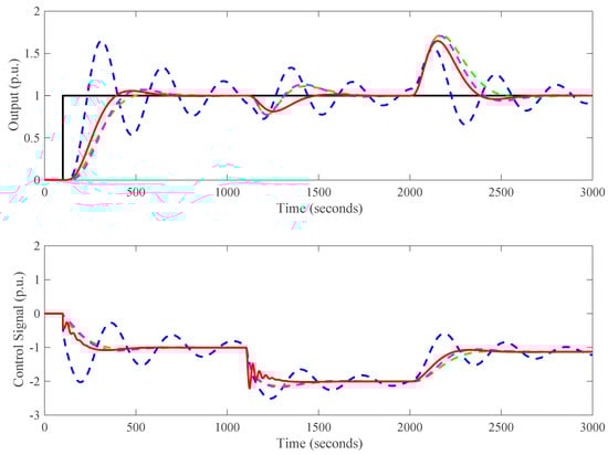
Figure 18.
Simulation results of SST system in the simulator with different control strategies. (Set point: —, PIsim-PI: - - -, PIi-PI: - - -, ADRC-PI: - - -, Hybrid ADRC: —).
Table 5.
Dynamic indices of SST system in the simulator with different control strategies.
As for Figure 18, we add sentences: ‘According to Figure 18, it is evident that the output of hybrid ADRC has the fastest tracking speed with small overshoot. Besides, compared with other cascade control strategies, the proposed strategy is able to reject the secondary disturbance more steadily and eliminate the deviation caused by the primary disturbance faster. This simulation results indicate the advantages of the hybrid ADRC in tracking and disturbance rejection. Similar to Section 4.2, we calculate the dynamic indices such as IAEsp, IAEud2 and IAEud1 in order to evaluate the performance of the proposed control strategy quantitatively. All these indices are listed in Table 5.
Compared with other three cascade control strategies, the proposed hybrid ADRC has best performance of tracking and disturbance rejection considering that its IAEsp, IAEud2 and IAEud1 are the smallest. Besides, the hybrid ADRC is able to reject the secondary disturbance steadily as well. The robustness test is essential for a control strategy so that Monte Carlo trials are carried out 500 times. In this subsection, time constants and gains in Equations (39) and (40) are perturbed within a range of ± 10%. Figure 19 shows the results of Monte Carlo trials.
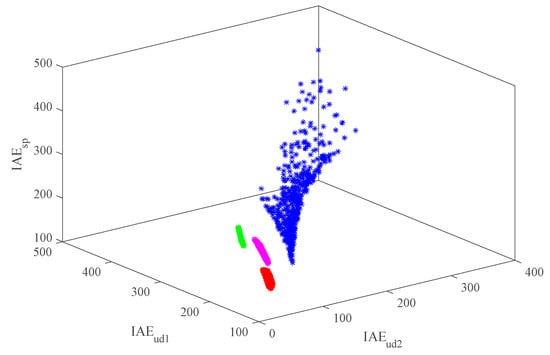
Figure 19.
Records of IAEsp, IAEud2 and IAEud1 for the perturbed SST system in the simulator. (PIsim-PI: *, PIi-PI: *, ADRC-PI: *, Hybrid ADRC: *)
From Figure 19, scatter points of the proposed hybrid ADRC are most intensive and they are nearest to the origin. Therefore, the hybrid ADRC is able to control the SST with stronger robustness and better dynamic performance compared with other comparative control strategies. Similar to Section 4.2, the ranges of dynamic indices are calculated in Table 6 to compare the robustness with different control strategies quantitatively.
Table 6.
Ranges of IAEsp, IAEud2 and IAEud1 of the perturbed SST system in the simulator.
According to Table 6, the hybrid ADRC has the narrowest ranges of IAEsp and IAEud2. Its range of IAEud1 is larger than that of PIi-PI but the former one has the smaller upper-lower limit. Therefore, the proposed has better robustness and dynamic performance.
Moreover, the sensitivity analysis of the multi-objective genetic algorithm is of significance for the reason that the identification results may influence the control performance. As a result, the population size and the number of generations are changed in this subsection in order to test the sensitivity of this optimization algorithm. Figure 20 shows the Pareto fronts of these cases.
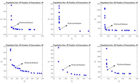
Figure 20.
Pareto fronts of different changed optimization parameters.
Table 7 shows the identification results of different cases. It is obvious that the dynamic parameters of these transfer functions are all in the perturbed range of dynamic parameters of Equations (39)–(40). Results of Monte Carlo trials indicate that the hybrid ADRC is able to obtain satisfactory control performance when SST is depicted as transfer functions illustrated in Table 7.
Table 7.
Identification results of different optimization cases.
5.2.3. Experiments on the Power Plant Simulator
Based on parameters given in Table 4, the hybrid ADRC is applied to the SST system of a 150 MW power plant simulator. In terms of field application, the bumpless switching of a controller is of importance. As for the hybrid ADRC, there are many state variables in its algorithm whose integration initial values should be set in order to implement the bumpless switching of the hybrid ADRC. Initial values of these state variables are set as:
where the superscript ‘*’ represents the last moment before the hybrid ADRC comes into service. Therefore, u*, y1* and y2* in Equation (41) are denoted as the valve opening, inlet temperature and SST at the moment aforementioned, respectively.
As for the implementation of the hybrid ADRC, the Euler method is used to calculate the numerical differentiation. The discrete compensation part is depicted as:
where h refers to the sampling step length and k is denoted as the current calculation step. According to Equation (13), the ESO is discretized as:
Similarly, the SFCL is rewritten as:
Based on Equations (42)–(44), the hybrid ADRC can be implemented on the DCS platform of the power plant simulator.
Moreover, the stability analysis of the hybrid ADRC provided in Section 3.3.1 is based on the general SST systems which means that if parameters of the controller are chosen appropriately the closed-loop system is stable. In this subsection, the parameters of the hybrid ADRC are tuned based on Figure 12.
Note that the operating point is about 100 MW. During the experiment, the set point of SST changes from 535 ℃ to 533 ℃ at 500 s and a 2% positive disturbance is added at the valve opening after the SST is stable at the set point. Figure 21 and Figure 22 show the experimental results of tracking and disturbance rejection, respectively.
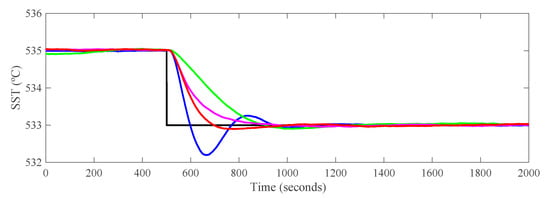
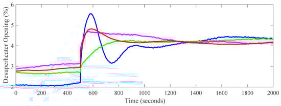
Figure 21.
Experimental results of tracking on the power plant simulator. (Set point: —, PIsim-PI: —, PIi-PI: —, ADRC-PI: —, Hybrid ADRC: —).
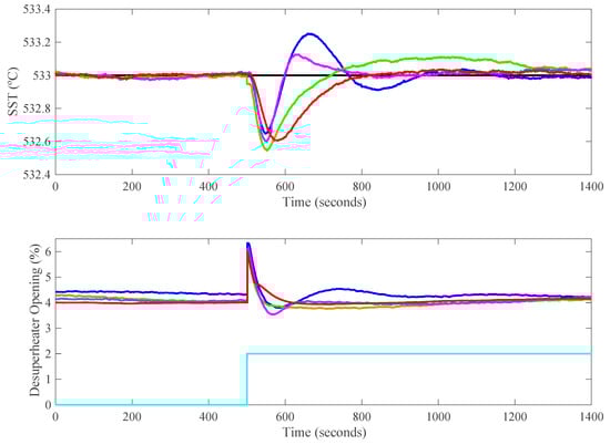
Figure 22.
Experimental results of disturbance rejection on the power plant simulator. (Set point: —, Disturbance: —, PIsim-PI: —, PIi-PI: —, ADRC-PI: —, Hybrid ADRC: —).
From Figure 21 and Figure 22, it is obvious that the proposed hybrid ADRC has better tracking performance and is able to reject the opening disturbance steadily. According to Figure 21, the output of the proposed hybrid ADRC is able to track the set point of SST faster than those of PIi-PI and ADRC-PI. Moreover, its overshoot is smaller than that of PIsim-PI. These mean that the hybrid ADRC has advantages in reference tracking. From Figure 22, the hybrid ADRC can reject the opening disturbance more steadily than other comparative control strategies which shows its superiority in disturbance rejection.
In this subsection, IAEud is defined as the IAE of rejecting the opening disturbance. Besides, in terms of disturbance rejection, the positive peak error (e+), the negative peak error (e−) and the average absolute error () are recorded as well. Table 8 illustrates the dynamic indices of different control strategies based on the experimental results.
Table 8.
Experimental dynamic indices of different control strategies.
According to Table 8, the hybrid ADRC has smallest IAEsp, e+ and . Although PIsim-PI has the smallest e-, its overshoot is larger than other three control strategies. Moreover, ADRC-PI shows its advantage in disturbance rejection but its tracking performance is worse than the hybrid ADRC.
Generally speaking, as for the control of SST, the hybrid ADRC is able to obtain satisfactory control performance and has simpler control structure than the cascade control strategy. Eventually, we make a comparison of our contributions in this work with those in [4,24,33]. New contributions are summarized as follows:
- All the SST control systems in [4,24,33] are cascade control systems. However, the SST control based on the hybrid ADRC is a single-loop control system which has the simpler structure.
- Compared with the different cascade control strategies in [4], the proposed hybrid ADRC is able to reject the secondary disturbance more steadily.
- The multi-objective optimization tuning method proposed in [24] requires a large amount of calculation. However, the tuning procedure of the hybrid ADRC is summarized as a flow chart in Section 4.1 which is easy to understand and use for engineers.
- As for the SST control systems proposed in [4,33], the MADRC and ADRC are designed as the outer-loop controller without considering the inner-loop transfer function G1(s). In this paper, the hybrid ADRC is designed based on both G1(s) and G2(s).
6. Conclusions
SST is a typical thermal process with sluggish response and its conventional cascade control structure is complex. In this paper, a single loop control strategy based on a hybrid ADRC is proposed in order to simplify the control structure and enhance the control performance. The stability analysis is conducted theoretically to guarantee the convergence of the hybrid ADRC. Besides, its ability to reject the secondary disturbance is discussed by the equivalent closed-loop block diagram. Then a practical tuning procedure for the hybrid ADRC is summarized to guide the tuning of its parameters. Based on the proposed tuning procedure, a numerical simulation is carried out to illustrate that the hybrid ADRC is able to improve the performance of tracking and disturbance rejection while its robustness is satisfactory. Finally, an experiment on a 150 MW power plant simulator is conducted to validate the advantages of the hybrid ADRC. Experimental results show that using the hybrid ADRC is able to enhance the control performance of SST while the structure of closed-loop system is simpler than that of the cascade control strategy. This successful application to the SST system of a power plant simulator indicates the promising prospect in the future field test of SST control based on the proposed single-loop control strategy.
The future work will focus on:
- The application of the hybrid ADRC to supercritical units and ultra-supercritical units.
- The frequency domain analysis of the hybrid ADRC.
- The development of the auto-tuning toolbox of the hybrid ADRC.
Author Contributions
Conceptualization, D.L.; Methodology, G.S., Z.W. and D.L.; Supervision, D.L. and Y.D.; Funding acquisition, D.L.; Validation, G.S., Z.W. and J.G.; Writing—original draft, G.S.; Writing—review & editing, G.S., Z.W., J.G., D.L. and Y.D. All authors have read and agreed to the published version of the manuscript.
Funding
This study was funded by the National Science and Technology Major Project 2017-V-0005-0055. This study also received financial support from the State Key Lab of Power Systems, Tsinghua University.
Acknowledgments
The authors would like to thank the support for technology and platform provided by Bernouly (Beijing) Simulation Technology Co., Ltd.
Conflicts of Interest
The authors declare no conflict of interest.
References
- Wu, Z.; Li, D.; Xue, Y.; Chen, Y. Gain scheduling design based on active disturbance rejection control for thermal power plant under full operating conditions. Energy 2019, 185, 744–762. [Google Scholar] [CrossRef]
- U.S. Energy Information Administration. International Energy Outlook 2013; U.S. Energy Information Administration: Washington, DC, USA, 2013.
- Liu, J.L.; Zeng, D.; Tian, L.; Gao, M. Control strategy for operating flexibility of coal-fired power plants in alternate electrical power systems. Proc. CSEE 2015, 35, 5385–5394. [Google Scholar]
- Wu, Z.; He, T.; Li, D.; Xue, Y.; Sun, L.; Sun, L.M. Superheated steam temperature control based on modified active disturbance rejection control. Control Eng. Pract. 2018, 83, 83–97. [Google Scholar] [CrossRef]
- Han, J. From PID to active disturbance rejection control. IEEE Trans. Ind. Electron. 2009, 56, 900–906. [Google Scholar] [CrossRef]
- Wu, X.; Shen, J.; Li, Y.G.; Lee, K.Y. Fuzzy modeling and predictive control of superheater steam temperature for power plant. ISA Trans. 2015, 56, 241–251. [Google Scholar] [CrossRef]
- Ma, L.Y.; Lee, K.Y. Neural network based superheater steam temperature control for a large-scale supercritical boiler unit. In Proceedings of the IEEE Power and Energy Society General Meeting, Detroit, MI, USA, 24–29 July 2011; pp. 1–8. [Google Scholar]
- Shome, A.; Ashok, S.D. Fuzzy logic approach for boiler temperature & water level control. Int. J. Sci. Eng. Res. 2012, 3, 1–6. [Google Scholar]
- Wu, Z.; Li, D.; Wang, L. Control of the superheated steam temperature: A comparison study between PID and fractional order PID controller. In Proceeding of the 35th Chinese Control Conference, Chengdu, China, 27–29 July 2016; pp. 10521–10526. [Google Scholar]
- Hou, Z.; Xiong, S. On model-free adaptive control and its stability anaylsis. IEEE Trans. Autom. Control 2019, 64, 4555–4569. [Google Scholar] [CrossRef]
- Roman, R.; Precup, R.; Bojan-Dragos, C.; Szedlak-Stinean, A. Combined model-free adaptive control with fuzzy component by virtual reference feedback tuning for tower crane systems. Procedia Comput. Sci. 2019, 162, 267–274. [Google Scholar] [CrossRef]
- Shi, G.; He, T.; Wu, Z.; Li, D. Research on cascade active disturbance rejection control of superheated steam temperature based on gain scheduling. In Proceedings of the 19th International Conference on Control, Automation and Systems, Jeju, Korea, 15–18 October 2019; pp. 1426–1431. [Google Scholar]
- Gao, Z. Scaling and bandwidth-parameterization based controller tuning. In Proceedings of the American Control Conference, Denver, CO, USA, 4–6 June 2003; pp. 4989–4996. [Google Scholar]
- Wu, Z.; Li, D.; Xue, Y.; Sun, L.M.; He, T.; Zheng, S. Modified active disturbance rejection control for fluidized bed combustor. ISA Trans. 2020, in press. [Google Scholar] [CrossRef]
- Zhang, J.; Feng, J.; Zhou, Y.; Fang, F.; Yue, H. Linear active disturbance rejection control of waste heat recovery systems with organic rankine cycles. Energies 2012, 5, 5111–5125. [Google Scholar] [CrossRef]
- Huang, C.; Li, D.; Xue, Y. Active disturbance rejection control for the ALSTOM gasifier benchmark problem. Control Eng. Pract. 2013, 21, 556–564. [Google Scholar] [CrossRef]
- Dong, Z.; Liu, M.; Jiang, D.; Huang, X.; Zhang, Y.; Zhang, Z. Automatic generation control of nuclear heating reactor power plants. Energies 2018, 11, 2782. [Google Scholar] [CrossRef]
- He, T.; Wu, Z.; Shi, R.; Li, D.; Sun, L.; Wang, L.; Zheng, S. Maximum sensitivity-constrained data-driven active disturbance rejection control with application to airflow control in power plant. Energies 2019, 12, 231. [Google Scholar] [CrossRef]
- Sun, L.; Jin, Y.; You, F. Active disturbance rejection temperature control of open-cathode proton exchange membrane fuel cell. Appl. Energy 2020, 261, 114381. [Google Scholar] [CrossRef]
- Xue, W.; Zhang, X.; Sun, L.; Fang, H. Extended state filter based disturbance and uncertainty mitigation for nonlinear uncertain systems with application to fuel cell temperature control. IEEE Trans. Ind. Electron. 2020. [Google Scholar] [CrossRef]
- Ramirez-Neria, M.; Gao, Z.; Sira-Ramirez, H.; Garrido-Moctezuma, R.; Luviano-Juarez, A. On the tracking of fast trajectories of a 3DOF torsional plant: A flatness based ADRC approach. Asian J. Control 2020. [Google Scholar] [CrossRef]
- Wu, C.; Song, K.; Li, S.; Xie, H. Impact of electrically assisted turbocharger on the intake oxygen concentration and its disturbance rejection control for a heavy-duty diesel engine. Energies 2019, 12, 3014. [Google Scholar] [CrossRef]
- Liang, G.; Li, W.; Li, Z. Control of superheated steam temperature in large-capacity generation units based on active disturbance rejection method and distributed control system. Control Eng. Practice 2013, 21, 268–285. [Google Scholar] [CrossRef]
- Sun, L.; Hua, Q.; Shen, J.; Xue, Y.; Li, D.; Lee, K.Y. Multi-objective optimization for advanced superheater steam temperature control in a 300 MW power plant. Appl. Energy 2017, 208, 592–606. [Google Scholar] [CrossRef]
- Xia, Y.; Liu, B.; Fu, M. Active disturbance rejection control for power plant with a single loop. Asian J. Control 2012, 14, 239–250. [Google Scholar] [CrossRef]
- Guo, B.Z.; Zhao, Z.L. On the convergence of an extended state observer for nonlinear systems with uncertainty. Syst. Control Lett. 2011, 60, 420–430. [Google Scholar] [CrossRef]
- Huang, Y.; Xue, W. Active disturbance rejection control: Methodology and theoretical analysis. ISA Trans. 2014, 53, 963–976. [Google Scholar] [CrossRef]
- Dorf, R.C.; Bishop, R.H. Modern Control System Eleventh Edition; Pearson Education, Inc.: Hoboken, NJ, USA, 2008. [Google Scholar]
- Wu, Z.; Zhang, F.; Shi, G.; He, T.; Li, D.; Chen, Y. Frequency-domain analysis of a modified active disturbance rejection control with application to superheated steam temperature control. In Proceedings of the 19th International Conference on Control, Automation and Systems, Jeju, Korea, 15–18 October 2019; pp. 44–50. [Google Scholar]
- Li, X.; Ding, D.; Wang, Y.; Huang, Z. Cascade IMC-PID control of superheated steam temperature based on closed-loop identification in the frequency domain. IFAC-PapersOnLine 2016, 49, 91–97. [Google Scholar] [CrossRef]
- Zhang, F.; Xue, Y.; Li, D.; Wu, Z.; He, T. On the flexible operation of supercritical circulating fluidized bed: Burning carbon based decentralized active disturbance rejection control. Energies 2019, 12, 1132. [Google Scholar] [CrossRef]
- Deb, K.; Agrawal, S.; Pratap, A.; Meyarivan, T. A fast elitist non-dominated sorting genetic algorithm for multi-objective optimization: NSGA-II. In Proceedings of the 6th International Conference on Parallel Problem Solving from Nature, Paris, France, 18–20 September; pp. 849–858.
- He, T.; Wu, Z.; Li, D.; Wang, J. A tuning method of active disturbance rejection control for a class of high-order processes. IEEE Trans. Ind. Electron. 2019, 67, 3191–3201. [Google Scholar] [CrossRef]


© 2020 by the authors. Licensee MDPI, Basel, Switzerland. This article is an open access article distributed under the terms and conditions of the Creative Commons Attribution (CC BY) license (http://creativecommons.org/licenses/by/4.0/).