Abstract
This study proposes a methodology to develop adaptive operational strategies of customer-installed Energy Storage Systems (ESS) based on the classification of customer load profiles. In addition, this study proposes a methodology to characterize and classify customer load profiles based on newly proposed Time-of-Use (TOU) indices. The TOU indices effectively distribute daily customer load profiles on multi-dimensional domains, indicating customer energy consumption patterns under the TOU tariff. The K-means and Self-Organizing Map (SOM) sophisticated clustering methods were applied for classification. Furthermore, this study demonstrates peak shaving and arbitrage operations of ESS with current supporting polices in South Korea. Actual load profiles accumulated from customers under the TOU rate were used to validate the proposed methodologies. The simulation results show that the TOU index-based clustering effectively classifies load patterns into ‘M-shaped’ and ‘square wave-shaped’ load patterns. In addition, the feasibility analysis results suggest different ESS operational strategies for different load patterns: the ‘M-shaped’ pattern fixes a 2-cycle operation per day due to battery life, while the ‘square wave-shaped’ pattern maximizes its operational cycle (a 3-cycle operation during the winter) for the highest profits.
1. Introduction
Smart grid circumstances employ various Internet of Thing (IoT) devices to provide efficient energy management for electric power consumers [1]. A smart meter is a representative IoT device that measures electrical energy data of customers in real time and transmits these data through network communication. Thus, the smart meter in a smart grid is utilized to collect electric load profiles of clients and enables electric power suppliers to identify the energy information of their clients [2,3]. In South Korea, the Korea Electric Power Corporation (KEPCO) acquires the electric load profiles of its customers and provides various electric energy statistics based on the accumulated load data through the ‘i-Smart’ platform [4].
The efficient analysis of customer load profiles can be effectively utilized to optimize energy management for all types of electricity customers. Clustering approaches are frequently used to efficiently analyze and classify different types of customer load profiles. Several studies have introduced methodologies to classify load profiles accumulated from different customer types. Motlagh et al. classified residential customers using characteristics of the time series load [5]. Chico et al. characterized and classified load profiles of non-residential customers using machine learning-based clustering algorithms [6]. Lee et al. classified the electric power consumption characteristics of industrial customers using the standard industry classification code in South Korea [7]. Bidoki et al. applied different clustering algorithms based on K-means, weighted fuzzy mean K-means, modified follow leader (MFTL), self-organizing map (SOM), and layer algorithm to classify load curves of different types of customers, and the results from comparing the clustering performances utilized to determine the adaptive clustering algorithms [8]. Zhou et al. proposed the five-stage process model based on K-means, SOM, Fuzzy c-average (FCM), and hierarchical clustering algorithms to analyze the impact of electric power suppliers and their consumers in smart grid circumstances [9]. Abubaker classified load profiles achieved from electricity consumers in the Tulkarm district based on the K-means algorithm [10].
These clustering-based approaches for analyzing customer load profiles can be applied to the development of effective strategies for energy management in smart grid circumstances. The representative strategy utilizes the Energy Storage System (ESS) installed for electricity consumers [11]. The ESS is a device that enables the storage of electrical energy during off-peak times and supplies the stored energy at the requested time to reduce electricity costs for the customer. The South Korean government had established a long-term roadmap and supporting policies to increase the penetration level of ESS, and, consequently, South Korea has been positioned as the second largest nameplate capacity of ESS since 2016 [12].
Several studies have proposed methodologies to optimize and develop operational strategies of ESS with consideration of the installation purposes and circumstances of the ESS. A pioneering study of applying the storage system to power utility showed optimization of the storage capacity based on the feasibility analysis of peak shaving [13]. Ehsan et al. developed charge and discharge scheduling of ESS based on the load forecasting model and state of charge (SOC) trajectory [14]. This approach shaved the peak load and smoothed the load connected with renewable energy sources. Pimm et al. proposed a method to determine the maximum peak shaving of household ESS using the Monte Carlo analysis, and the results confirmed the capacity to reduce the household peak demand by 50% [15]. Karmiris et al. estimated the optimal size of ESS based on the capabilities of its peak shaving operation and scheduled adaptive charging and discharging scenarios using statistical analysis [16]. Dejvises et al. proposed a mathematical modeling for ESS to minimize daily peak loads for customers, and this approach showed a 7.4% reduction of the daily peak load with a 9.9% increase of its daily load factor [17]. Reza et al. introduced the gradient-based heuristic optimization algorithm to calculate the optimal charge and discharge schedule of ESS for maximizing the expected profit from the ESS operation [18]. Kang et al. developed the operational strategy for customer-installed ESS to participate in the Demand Response (DR) program in South Korea [19]. They also provided guidelines to facilitate ESS participation in the DR program. Cha et al. proposed an algorithm considering system marginal price (SMP) and renewable energy certification (REC) weight for the economical optimal scheduling of ESS [20].
Previous researches have verified that customer-installed ESS and its supporting policies of government and utility levels are feasible for electricity customers that use the Time-of-Use (TOU) tariff structure. In addition, the literature has also indicated that optimization of ESS operational strategies should be differentiated depending on the energy demand (electrical load) pattern of its installation site as well as consideration of the customer tariff and the battery constraints. The literature has also verified that the clustering of customer load profiles can be effectively utilized to optimize energy management for different types of electricity customers. Thus, this study proposes a methodology to develop adaptive operational strategies of customer-installed ESS in accordance with classified results of load profiles for customers using the TOU tariff structure. In addition, this study proposes a methodology to characterize and classify the load profiles based on newly proposed TOU indices. The TOU indices enable the effective distribution of daily customer load profiles on multi-dimensional domains, indicating characteristics of the customer’s energy consumption pattern under the TOU tariff. The K-means and Self-Organizing Map (SOM) sophisticated clustering methods are applied for classification. Furthermore, this study demonstrates benefits of peak shaving and arbitrage operations of customer-installed ESS with current supporting polices in South Korea. The proposed methodologies are validated by simulations based on actual load profiles accumulated by industries and commercial buildings. The simulation results show that TOU index-based clustering effectively classifies load patterns into ‘M-shaped’ (industries) and ‘square wave-shaped’ load patterns (commercial buildings). In addition, the feasibility analysis results suggest different operational strategies of ESS for different clusters grouped together by a similar load pattern.
The rest of this paper is organized as follows. Section 2 proposes the TOU indices and the classification methodologies based on the proposed TOU indices. Section 3 introduces the ESS supporting polices in South Korea and operational algorithms of customer-installed ESS, including peak shaving and arbitrage operations. Section 4 simulates the proposed methodologies based on the actual TOU customer load profiles and performs a feasibility study to derive an optimized ESS operational strategy. Finally, the paper is concluded in Section 5.
2. Clustering
2.1. TOU Indices
This paper proposes new TOU indices developed based on seasonal and temporal characteristics of the TOU tariff structure in South Korea for efficient classification of customers’ load profiles. The KEPCO offers a TOU tariff structure for industrial and commercial customers, which charges differently in different seasons of the year and different classifications in a day. Table 1 shows the daily TOU rate schedules separated by two seasons: non-winter (spring, summer, and fall) and winter. For each season, the 24-hour schedule on weekdays is classified into three different levels of electric power consumption: off-peak, mid-peak, and on-peak load. The on-peak load is substituted by the mid-peak load on Saturdays. The only off-peak load is chargeable on Sundays and national holidays. In addition, the TOU tariff depends on the demand charge rate () and the usage charge rate ().

Table 1.
Daily TOU rate schedules [21].
Table 2 shows two examples of a TOU tariff: Industrial Service B (High-Voltage B) and General Service B (High-Voltage A) [21]. The tariff is classified into Industrial and General depending on the customer type. The Service B indicates that the customer’s contract demand is above 300 kW. The voltage connected to the grid decides the High-Voltage such as 3.3–66 kV for High-Voltage A and 154 kV for High-Voltage B. The selectable options of this tariff indicate that a relatively higher consists of a lower , and, thus, customers could choose a suitable option depending on their consumption patterns. The comparison between Industrial and General in Table 2 shows an identical structure with small variations of and depending on options. This indicates that the energy demand pattern can be one of the determinative factors to develop adaptive strategies of energy management for customers.
Table 2.
Examples of a TOU tariff [21].
The monthly electric charge () of industrial and commercial customers is calculated as follows [21]:
where is the annually highest value of the customer load profile, is the energy consumption of the customer, and 1.137 indicates 10% of VAT and 3.7% of the Electric Power Industry Basis Fund.
Based on this tariff structure, this study proposes TOU indices consisting of an off-peak index (), mid-peak index (), and on-peak index (). These are calculated as follows:
where , and each are the time duration of off-peak (10 hours), mid-peak (8 hours), and on-peak (6 hours). , and are the average levels of electric power consumption during off-peak, mid-peak, and peak load times, respectively. The TOU indices show the power consumption rates according to the TOU time schedule and compares the daily total power consumption between the daily load profiles. Therefore, TOU indices can be classified according to the customer load pattern, which they are expected to utilize to establish an effective ESS control strategy.
2.2. Evaluation Parameter
For internal evaluation of clustering, the Davies-Bouldin Index (DBI) and the Silhouette Index (SI) are used to determine an optimal number of clusters [22]. DBI indicates the ratio of the cohesion in a cluster to the separation between different clusters. The cohesion observes the distance between a center point of a cluster and the data of the corresponding cluster, and the separation calculates the distance between the center points of different clusters. DBI is calculated as follows [23]:
where N is the number of clusters, is the distance between the center points of cluster i and cluster j, is the average distance between the center point of cluster i and the data of the cluster i, is the average distance between the center point of cluster j and the data of the cluster j.
SI observes the average distance between the nth data and the other data in the identical cluster and the average distance between the nth data and all data of different clusters. It is calculated as follows [24]:
where k is the number of all data, is the average distance between the nth data and the other data of the identical cluster, and is the smallest value of the average distances between the nth data and all data of the other clusters.
The lower DBI and higher SI values expect higher cohesion in the selected cluster and higher separation of the other clusters. Thus, this study observes the changes of DBI and SI according to the changes of the cluster number, and the optimal number of the cluster is decided when the value of subtracting DBI from SI is the highest for satisfying both the lowest DBI and the highest SI.
The Adjusted Rand Index (ARI) is used to externally evaluate clustering performance through similarities between the clustering results and the target cluster. This verifies the similarities between the target cluster and the clustering result based on the number of matching data ARI is proposed to improve the Rand Index (RI), the ratio of the number of correct data pairs to the number of all possible data pairs [25]. Table 3 shows a contingency table for comparing between the target cluster and the clustering result . is the number of matching data between and . is the number of data in , and is the number of data in . First of all, RI is calculated as follows [25]:
where is the number of pairs are included in the same class in and in the same cluster in , is the number of pairs are included in different classes in and in different clusters in , is the number of pairs are included in the same class in and in different clusters in , and is the number of pairs are included in different classes in and in the same cluster in . This ranges from 0 to 1, and 1 is considered as the best performance. ARI modifies the limitations of RI such as no constant value of the expected value of the RI and the upper limit approaches as increasing the number of clusters, which is calculated as follows [25]:
Table 3.
Notation for comparing the target cluster and the clustering result .
The clustering performance based on ARI can be evaluated as ‘excellent’ when ARI ≥ 0.9, ‘good’ when 0.8 ≤ ARI < 0.9, ‘moderate’ when 0.65 ≤ ARI < 0.8, and ‘poor’ when ARI < 0.65 [26].
2.3. Clustering Methodology
This paper distributes daily load profiles of customers based on the TOU indices in a multi-dimensional manner. These index-based distributions are classified into three different day types: Weekdays (Non-winter), Weekdays (Winter), and Saturdays. The weekdays need to be separated into non-winter and winter according to the seasonal classification of the TOU tariff structure as described in Table 1. Saturdays are also separately observed since the tariff substitutes the on-peak load with the mid-peak load. Sundays and holidays are excluded since the tariff only applies to the off-peak rate.
The distributed data on weekdays (non-winter and winter) and on Saturdays are classified by using sophisticated clustering methods: K-means and Self-Organizing Map (SOM). First, the K-means algorithm is one of the most frequently utilized approaches for clustering. Given a dataset of and a cluster set , this algorithm obtains the minimum distance between input data and center points of the clusters, calculated as follows [27]:
where is the nth input data in and is the center point of nth cluster in .
This study also utilizes SOM, a clustering technique based on Artificial Neural Networks (ANNs). The SOM algorithm classifies data into the nearest neurons by calculating the distance between the data input of the input layer and the neurons of the output layer [28]. First, the Euclidean distance between the input data and the weight of output neuron is achieved to determine the nearest neuron as the winner neuron W, calculated as follows [29]:
where is the output neuron vector at the number of iterations t, and is the input data. The determined winner neuron W is updated by the following steps [29]:
where is the Gaussian neighborhood function, is the coordinate position of the neuron, is the learning rate, and is the width of the neighborhood radius.
3. Customer-Installed ESS
3.1. Supporting Policies
The Korean government and KEPCO have established ESS supporting policies to encourage customers to install ESS to stabilize the national electric power system and to reduce and stabilize greenhouse gas emissions [30]. These policies are classified into demand and usage charge discounts. The demand charge discount compensates for the monthly contribution of ESS discharge during on-peak hours. This monthly contribution () is calculated as follows [21]:
where and are the sum of discharge and charge energy of ESS, respectively, during the on-peak load hours on weekdays of the corresponding month, and is the number of the weekdays of the corresponding month. Finally, the KEPCO offers to subtract from of the Equation (1), and, consequently, customers save their demand charge on the monthly electricity bill. The usage charge discount provides a 50% discount of the customers’ usage charge when ESS charges its energy during off-peak load hours [21].
3.2. Operational Algorithm
The operational algorithm of customer-installed ESS is divided into a peak shaving operation and an arbitrage operation. The peak saving operation reduces an annual peak load of customers with discharge of their ESS. This algorithm sets the peak reference based on consideration of ESS capabilities of energy storage and charge/discharge rates, and the ESS maintains the annual peak to not exceed the peak reference. The arbitrage utilizes differences of energy usage charge rates. This algorithm saves the customers’ energy usage charge by charging their ESS during the hours of the relatively lower usage charge rate and then discharging the energy during the hours of the relatively higher usage charge rate [29]. The daily charge-discharge cycles for the arbitrage operation can be selected to a single cycle (1-cycle) or multiple cycles depending on the TOU schedules. The South Korean TOU tariff structure is divided into on-peak (highest rate), mid-peak, and off-peak (lowest rate) load hours as described in Table 2. According to the rate schedules in Table 1, the daily maximal arbitrage cycle is two on weekdays in non-winter (morning off-peak and on-peak discharging and afternoon mid-peak and on-peak discharging) and three on weekdays in winter (morning off-peak charging and on-peak discharging, afternoon mid-peak and on-peak discharging, and night mid-peak and on-peak discharging).
Figure 1 shows a flowchart of the operational strategy of customer-installed ESS using the peak shaving and arbitrage operations with different daily charge-discharge cycles in South Korea. These strategies commonly prioritize peak shaving operations compared to arbitrage operations, since the demand charge saving from peak shaving is more efficient than the energy charge saving from arbitrage [31]. Dozens of days are usually expected to exceed the peak reference during a year. For these days, the single-cycle operation performs the only peak shaving as shown in Figure 1a. However, the multi-cycle operations can choose the full peak shaving or the combined operation of the early peak shavings and the late arbitrages when late arbitrages are available after finishing the peak shaving as described in Figure 1b,c. For the other days not exceeding the peak reference, the ESS only performs the arbitrage operation. For these days, the multi-cycle operations can choose merely the 2-cycle operation for all weekdays (Figure 1b) or the 2-cycle for weekdays in non-winter and the 3-cycle for weekdays in winter (Figure 1c).
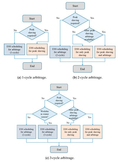
Figure 1.
A flowchart of the operational strategy of ESS under the TOU tariff structure in South Korea: (a) 1-cycle, (b) 2-cycle, and (c) 3-cycle arbitrage.
Figure 2 shows examples of daily charges and discharges of ESS installed in an industrial customer. The daily load pattern of this customer shows the typical M-shaped pattern, and the total capacity of the ESS is assumed to be 10% of the customer annual peak load with a 1C-rate capability. First of all, the ESS always charges its energy during the earliest off-peak load hours, the cheapest usage charge duration, for all three cases. In Figure 2a, the ESS discharges the charged energy for the peak shaving operation when the customer load exceeds the peak reference both in the morning (10:00 ~ 12:00) and afternoon (13:00 ~ 17:00). Figure 2b shows the combined operation of peak shaving and arbitrage on a weekday in winter. On this day, the ESS discharges to handle the customer load that exceeds the peak reference between 11:00 and 12:00, and it discharges the remaining energy during the second term of on-peak load hours (17:00 ~ 20:00) for the arbitrage operation. In addition, the ESS performs an additional arbitrage operation that charges the energy during mid-peak load hours (20:00 ~ 22:00) and discharges the energy during the third term of on-peak load hours (22:00 ~ 23:00). Figure 2c shows the arbitrage operation with 2-cycle on a weekday in non-winter. The ESS operates its first discharging during the morning on-peak load hours (10:00 ~ 12:00). In addition, it also performs the second charging during mid-peak load hours (12:00 ~ 13:00) and the corresponding discharging during the afternoon on-peak load hours (13:00 ~ 17:00). Figure 2d demonstrates the arbitrage operation with 3-cycle on a weekday in winter. The first discharging is identical to the 2-cycle arbitrage, but the second cycle is performed by charging during the mid-peak load hours (12:00 ~ 17:00) and discharging during the afternoon on-peak load hours (17:00 ~ 20:00). In addition, the ESS charges during the night mid-peak (20:00 ~ 22:00) and then discharges during the last on-peak (22:00 ~ 23:00) for the third arbitrage cycle.
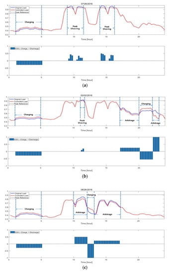
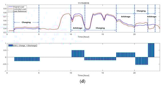
Figure 2.
Examples of Daily ESS operations: (a) only peak shaving, (b) combined operation of peak shaving and arbitrage, (c) only arbitrage with 2-cycle, and (d) only arbitrage with 3-cycle.
4. Simulation
4.1. Load Profile
The simulation utilizes actual load profiles accumulated by four different customers (Customers A, B, C, and D) using the TOU tariff structure. These load profiles are 15-minute-based data measurements by KEPCO from January 1 to December 31, 2016. In addition, the load profiles are normalized by their peak load for effective comparison of the customers. Figure 3 shows normalized seasonal average load profiles for Customers A, B, C, and D for (a) weekdays (non-winter), (b) weekdays (winter), (c) Saturdays, and (d) Sundays and holidays. In the case of weekdays, the daily averaged loads of Customers A and B show the ‘M-shaped’ pattern, the representative profile of manufacturing industries, while the daily averaged loads of Customers C and D show the ‘square wave-shaped’ pattern, the typical profile of commercial buildings. Customers A and B use Industrial Service B (High-Voltage B, Option Ⅱ) and Customers C and D use General Service B (High-Voltage A, Option II).
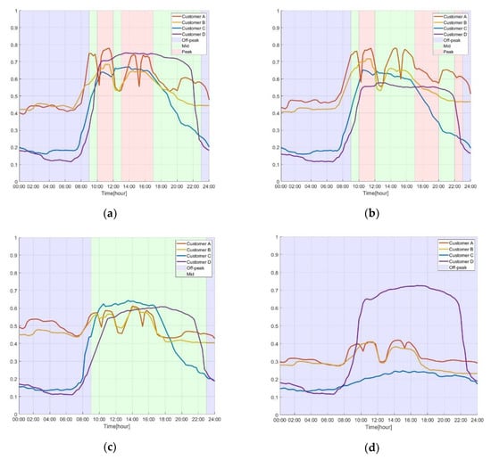
Figure 3.
Normalized seasonal average load profiles of the customers: (a) Weekdays (Non-winter), and (b) Weekdays (Winter), (c) Saturdays, and (d) Sundays & Holidays.
4.2. Clustering Result
4.2.1. K-means
The internal evaluation parameters based on the K-means approach are observed to determine the optimal cluster number. Table 4 shows DBI, SI, and DBI-SI values by increasing the cluster number from 2 to 5. The optimal cluster number is selected to be 2, since the cluster number 2 shows the highest values of SI-DBI for Weekdays (non-winter), Weekdays (winter), and Saturdays. Figure 4 shows the clustering result of the K-means approach when the cluster number is 2. This demonstrates that most data from Customers A and B are classified into Cluster 1, otherwise, most data from Customers C and D are classified into Cluster 2 for Weekdays (Non-winter), Weekdays (Winter), and Saturdays. Table 5 shows the ARI-based external evaluation of K-means when the cluster number is 2. The total ARI value is calculated to 0.919, which can be evaluated as the ‘excellent’ clustering result. Figure 5a describes the separated data distributions of Clusters 1 and 2 for Weekdays (Non-winter) with 0.890 of the ARI value, which can be evaluated as the ‘good’ result. The results of Weekdays (Winter) show the relatively lower ARI value (0.797) compared to that of Weekdays (Non-winter). This is due to the relatively closer center points between Clusters 1 and 2 as described in Figure 5b, and, consequently, the failure rate of clustering is relatively increased. For Saturdays, Figure 5c indicate a significant separation between the two clusters with the highest ARI values (0.942).
Table 4.
Internal evaluation indices at different cluster numbers based on K-means.
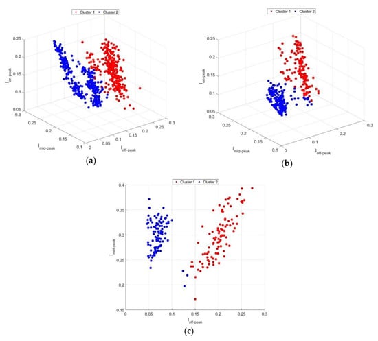
Figure 4.
K-means clustering result: (a) Weekdays (Non-winter), (b) Weekdays (Winter), and (c) Saturdays.
Table 5.
External evaluation results of K-means.
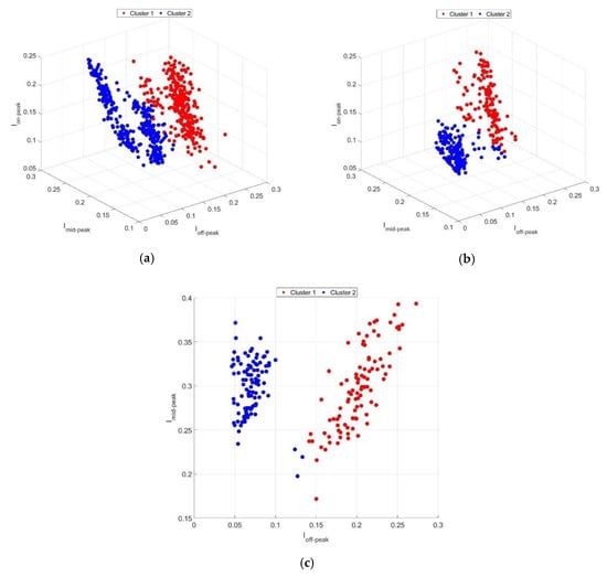
Figure 5.
SOM clustering result: (a) Weekdays (Non-winter); (b) Weekdays (Winter); (c) Saturdays.
4.2.2. SOM
This study observes DBI, SI, and SI-DBI values based on the SOM approach by varying the cluster dimension (2 × 1, 3 × 1, 4 × 1, 2 × 2, and 5 × 1) summarized in Table 6. Similar with the K-means approach, the optimal cluster dimension for SOM is selected as 2 × 1, the highest values of SI-DBI for all three cases. Figure 5 shows the SOM-based clustering result when the cluster dimension is 2 × 1. The SOM clustering results similarly shows the K-means-based clustering results, which groups Customers A and B into Cluster 1 and Customers C and D into Cluster 2. Table 7 shows the ARI-based external evaluation of SOM when the cluster dimension is 2 × 1. These results show the similar pattern of the K-means results in Table 4: the highest on Saturdays and the lowest on Weekdays (Winter). In addition, the total result of the SOM (0.922) shows a slightly improved performance compared to that of the K-means (0.919). Finally, the ARI-based external evaluation of both the K-means and SOM indicates an acceptable clustering performance.
Table 6.
Internal evaluation indices at different cluster numbers based on the SOM.
Table 7.
External evaluation results of SOM.
4.3. Feasibility Study
This study performs simulations for feasibility analysis of Customers A, B, C, and D to find their optimized ESS operational strategies. All simulations estimate that the customers have installed ESS with a capacity of 10% of their annual peak demand and a capability of 1 C-rate [19]. The ESS efficiency is assumed to be 91% for charging and 99% for discharging, and, consequently, the charge-discharge round-trip efficiency is calculated as approximately 90% [19]. The ESS is assumed to be a lithium-ion battery type with a life of 4000 cycles [32]. Thus, the battery lifespan is calculated as approximately 13 years with a 7.5% annual degradation for the single-cycle operation. However, the lifespan is reduced for the multi-cycle operation: approximately 7.2 years with a 13.75% annual degradation for a 2-cycle operation and 6.6 years with a 15% annual degradation for a 3-cycle operation. The ESS installation cost is selected to 500,000 [KRW/kWh], and its annual maintenance is considered to be 3% of the installation cost with 4.5% of the discount rate [33]. The supporting policies described in Section 3.1 are considered.
All simulations observe a net present value (NPV) for the feasibility analysis of each case, calculated as follows [34]:
where is the life span of the installed ESS, is the ESS installation cost, is the expected saving of the customer’s electricity charge, is the operation and maintenance costs, and r is discount rate. In addition, this study separately observes the expected unit saving [KRW/kWh] by the peak saving operation () and by the arbitrage operation ().
Table 8 summarizes the feasibility analysis results of Customers A, B, C, and D for their different cycle operations (1-cycle, 2-cycle, and 3-cycle). The results indicate that the multi-cycle (2-cycle and 3-cycle) operations expect relatively higher unit savings ( and ) and NPVs for all customers. This is due to the increased cycles not only improving their usage charge savings by increasing the arbitrages but also allowing a greater cut of their annual peaks, which increases savings in demand charges. In addition, the increased cycles also improve the monthly contribution () of the supporting policy in Equation (12).
Table 8.
Feasibility analysis results of the customer-installed ESS.
However, the results show different feasible solutions depending on the different clusters. First, the customers corresponding to Cluster 1 (Customers A and B) show a relatively higher improvement of the unit savings of the peak saving () between single- and multi-cycle operations compared to the customers corresponding to Cluster 2 (Customers C and D). This indicates that the M-shaped pattern of Cluster 1 expects a relatively deeper peak shaving from the multi-cycle operation compared to the square-wave shaped patten of Cluster 2. In addition, Customers A and B (Cluster 1) show the highest NPV for a 2-cycle arbitrage while Customers C and D (Cluster 2) show the highest NPV for a 3-cycle arbitrage. This is due to the M-shaped pattern of Cluster 1 expecting relatively lower unit savings from the arbitrage operation (CPBar) for both 2- and 3-cycle arbitrages compared to the square-wave shaped patten of Cluster 2. Thus, these results suggest that the 2-cycle arbitrage is enough for Cluster 1 with consideration of the battery’s life cycle, and the maximal cycle arbitrage is expected to maximize profits of the customer-installed ESS for Cluster 2.
5. Conclusions
This study proposes a methodology to develop the optimized operational strategy of customer-installed ESS depending on the cluster derived from the classification of load profiles under the TOU tariff structure. In addition, this study also proposes a methodology to characterize and classify the customer load profiles based on the newly proposed TOU indices consisting of off-peak, mid-peak, and on-peak indices. These indices enable the effective distribution of daily customer load profiles on multi-dimensional domains, indicating characteristics of the power consumption rates according to the TOU tariff schedule. Sophisticated clustering methods (K-means and SOM) are applied for classification. Furthermore, this study demonstrates the operational algorithms for the peak shaving and arbitrage of customer-installed ESS and the expected benefits for customers under the TOU tariff with current supporting polices in South Korea.
The proposed methodologies are validated by simulations based on actual load profiles accumulated from two different industries (Customers A and B) and two different commercial buildings (Customers C and D). The TOU index-based clustering results of both the K-means and SOM show an effective classification between the cluster of the ‘M-shaped’ load pattern (Customers A and B) and the cluster of the ‘square wave-shaped’ load pattern (Customers C and D). In addition, the feasibility analysis results suggest different operational strategies of ESS for different clusters. Daily 2-cycle operations are suggested for the customers included in the cluster of the ‘M-shaped’ load patterns (Cluster 1) due to consideration of the battery’s life cycle. However, the customers included in the cluster of the ‘square wave-shaped’ load pattern (Cluster 2) are required to employ daily maximal cycle operations (3-cycle operations) of ESS to maximize savings of customer electricity costs.
This research provides an early-stage methodology to develop adaptive solutions for multiple customers based on the clustering of the customer load profiles. The proposed methodologies will be advanced with extended load profiles, including more diverse patterns acquired from increased number of customers. This effort will contribute to the development of more advanced strategies of energy management improving profits of customer-installed ESS. In addition, the proposed methodologies and analysis results in this study are expected to provide guidelines to establish and modify related policies of government, utility, and aggregator levels.
Author Contributions
H.C.J. mainly performed the algorithm development and simulations. J.J. contributed to algorithm development and data acquisition. B.O.K. provided the guidelines of this research and assisted as an advising professor. All authors have read and agreed to the published version of the manuscript.
Funding
This research was supported by Korea Electric Power Corporation (Grant number: R18XA06-57).
Conflicts of Interest
The authors declare no conflict of interest.
References
- Lloret, J.; Tomas, J.; Canovas, A.; Parra, L. An Integrated IoT Architecture for Smart Metering. IEEE Commun. Mag. 2016, 54, 50–57. [Google Scholar] [CrossRef]
- Hernandez, L.; Baladrón, C.; Aguiar, J.M.; Carro, B.; Sánchez-Esguevillas, A.; Lloret, J.; Chinarro, D.; Gomez-Sanz, J.J.; Cook, D. A multi-agent system architecture for smart grid management and forecasting of energy demand in virtual power plants. IEEE Commun. Mag. 2013, 51, 106–113. [Google Scholar] [CrossRef]
- Lee, Y.; Hwang, E.; Choi, J. A Unified Approach for Compression and Authentication of Smart Meter Reading in AMI. IEEE Access 2019, 7, 34383–34394. [Google Scholar] [CrossRef]
- Yang, H. [KEPCO] Implementation of next-generation power portal service ‘i-SMART’. Electr. Power 2011, 52, 39. [Google Scholar]
- Motlagh, O.; Berry, A.; O’Neil, L. Clustering of residential electricity customers using load time series. Appl. Energy 2019, 237, 11–24. [Google Scholar] [CrossRef]
- Chicco, G.; Napoli, R.; Piglione, F. Application of clustering algorithms and self organising maps to classify electricity customers. In Proceedings of the 2003 IEEE Bologna Power Tech Conference Proceedings, Bologna, Italy, 23–26 June 2003; IEEE: Piscataway, NJ, USA, 1963; pp. 23–26. [Google Scholar]
- Lee, S.E.; Chung, C.T.; Lee, S.B. Electric consumption analysis using Korea Standard Industrial Classification Code. In Proceedings of the Korean Institute of Electrical Engineers Summer Conference, Yongpyong, Korea, 16–18 July 2014; pp. 471–472. [Google Scholar]
- Bidoki, S.M.; Kohan, N.M.; Gerami, S. Comparison of several clustering methods in the case of electrical load curves classification. In Proceedings of the 16th Electrical Power Distribution Conference, Bandar Abbas, Iran, 19–20 April 2011; pp. 1–7. [Google Scholar]
- Zhou, K.L.; Yang, S.L.; Shen, C. A review of electric load classification in smart grid environment. Renew. Sustain. Energy Rev. 2013, 24, 103–110. [Google Scholar] [CrossRef]
- AbuBaker, M. Data Mining Applications in Understanding Electricity Consumers’ Behavior: A Case Study of Tulkarm District, Palestine. Energies 2019, 12, 4287. [Google Scholar] [CrossRef]
- Manz, D.; Piwko, R.; Miller, N. Look before you leap: The role of energy storage in the grid. IEEE Power Energy Mag. 2012, 10, 75–84. [Google Scholar]
- United States Department of Energy. DOE Global Energy Storage Database. Available online: https://www.energystorageexchange.org/projects/data_visualization (accessed on 23 September 2017).
- Sobieski, D.W.; Bhavaraju, M.P. An economic assessment of battery storage in electric utility systems. IEEE Trans. Power Appar. Syst. 1985, 104, 3453–3459. [Google Scholar]
- Reihani, E.; Motalleb, M.; Ghorbani, R.; Saoud, L.S. Load peak shaving and power smoothing of a distribution grid with high renewable energy penetration. Renew. Energy 2016, 86, 1372–1379. [Google Scholar] [CrossRef]
- Pimm, A.J.; Cockerill, T.T.; Taylor, P.G. The potential for peak shaving on low voltage distribution networks using electricity storage. J. Energy Storage 2018, 16, 231–242. [Google Scholar] [CrossRef]
- Karmiris, G.; Tomas, T. Peak Shaving Control Method for Energy Storage; Corporate Research Center: Vasterås, Sweden, 2013. [Google Scholar]
- Dejvises, J. Energy storage system sizing for peak shaving in Thailand. ECTI Trans. Electr. Eng. Electron. Commun. 2016, 14, 49–55. [Google Scholar]
- Arghandeh, R.; Woyak, J.; Onen, A.; Jung, J.; Broadwater, R.P. Economic optimal operation of Community Energy Storage systems in competitive energy markets. Appl. Energy 2014, 135, 71–80. [Google Scholar] [CrossRef]
- Kang, B.O.; Lee, M.; Kim, Y.; Jung, J. Economic analysis of a customer-installed energy storage system for both self-saving operation and demand response program participation in South Korea. Renew. Sustain. Energy Rev. 2018, 94, 69–83. [Google Scholar] [CrossRef]
- Cha, H.J.; Lee, S.E.; Won, D. Implementation of Optimal Scheduling Algorithm for Multi-Functional Battery Energy Storage System. Energies 2019, 12, 1339. [Google Scholar] [CrossRef]
- Korea Electric Power Corp. Electrical Supply Terms and Conditions. Available online: http://cyber.kepco.co.kr (accessed on 19 October 2019).
- Lee, K.M.; Lee, K.M.; Lee, C.H. Statistical cluster validity indexes to consider cohesion and separation. In Proceedings of the 2012 International Conference on Fuzzy Theory and Its Applications (iFUZZY2012), Taichung, Taiwan, 16–18 November 2012; pp. 228–232. [Google Scholar]
- Lu, S.; Lin, G.; Liu, H.; Ye, C.; Que, H.; Ding, Y. A Weekly Load Data Mining Approach Based on Hidden Markov Model. IEEE Access 2019, 7, 34609–34619. [Google Scholar] [CrossRef]
- Liu, Y.; Li, Z.; Xiong, H.; Gao, X.; Wu, J. Understanding of Internal Clustering Validation Measures. In Proceedings of the 2010 IEEE International Conference on Data Mining, Sydney, NSW, Australia, 13–17 December 2010; pp. 911–916. [Google Scholar]
- Yeung, K.Y.; Ruzzo, W.L. Details of the Adjusted Rand index and Clustering Algorithms Supplement to the paper “An empirical study on Principal Component Analysis for clustering gene expression data” (to appear in Bioinformatics). Bioinformatics 2001, 17, 763–774. [Google Scholar] [CrossRef]
- Doreian, P.; Batagelj, V.; Ferligoj, A. Advances in Network Clustering and Blockmodeling, 1st ed.; Wiley: Hoboken, NJ, USA, 1807; p. 199. [Google Scholar]
- Jain, A.K. Data clustering: 50 years beyond K-means. Pattern Recognit. Lett. 2010, 31, 651–666. [Google Scholar] [CrossRef]
- Vesanto, J.; Alhoniemi, E. Clustering of the self-organizing map. IEEE Trans. Neural Netw. 2000, 11, 586–600. [Google Scholar] [CrossRef]
- Chaudhary, V.; Bhatia, R.S.; Ahlawat, A.K. A novel Self-Organizing Map (SOM) learning algorithm with nearest and farthest neurons. Alex. Eng. J. 2014, 53, 827–831. [Google Scholar] [CrossRef]
- Lee, S. Analysis of Energy Storage System (ESS) Demand Management Effect and Research on Market Formation Plan; Korea Energy Economics Institute: Ulsan, Korea, 2014. [Google Scholar]
- Kang, B.O.; Hwang, B.G.; Kwon, K.; Jung, J. Operational Strategy of Energy Storage System (ESS) to Participate in Demand Response (DR) Market for Industrial Customer. New Renew. Energy 2017, 13, 4–12. [Google Scholar] [CrossRef]
- Majima, M.; Ujiie, S.; Yagasaki, E.; Koyama, K.; Inazawa, S. Development of long-life lithium ion battery for power storage. J. Power Sources 2001, 101, 53–59. [Google Scholar] [CrossRef]
- Jeon, S.; Kim, Y.K.; Jung, J.; Kim, S. Feasibility Analysis of Tariff System for the Promotion of Energy Storage Systems (ESSs). New Renew. Energy 2019, 15, 69–76. [Google Scholar] [CrossRef]
- Park, J.; Heo, J.; Shin, S.; Kim, H. Economic Evaluation of ESS in Urban Railway Substation for Peak Load Shaving Based on Net Present Value. J. Electr. Eng. Technol. 2017, 12, 981–987. [Google Scholar] [CrossRef][Green Version]


© 2020 by the authors. Licensee MDPI, Basel, Switzerland. This article is an open access article distributed under the terms and conditions of the Creative Commons Attribution (CC BY) license (http://creativecommons.org/licenses/by/4.0/).